
You are currently browsing the tag archive for the ‘Dyson Brownian motion’ tag.
Let 

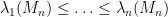


for any test function 

![{[x_1,x_1+\epsilon],\ldots,[x_k,x_k+\epsilon]}](https://s0.wp.com/latex.php?latex=%7B%5Bx_1%2Cx_1%2B%5Cepsilon%5D%2C%5Cldots%2C%5Bx_k%2Cx_k%2B%5Cepsilon%5D%7D&bg=ffffff&fg=000000&s=0&c=20201002)


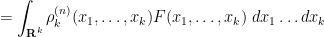
As is well known, the GUE process is a determinantal point process, which means that

for some kernel 
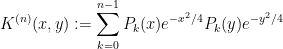
where 
Using the asymptotics of Hermite polynomials (which then give asymptotics for the kernel 


where 
A bit more precisely, for any fixed bulk energy 


On the other hand, an important feature of the GUE process 

which describes the stochastic evolution of eigenvalues of a Hermitian matrix under independent Brownian motion of its entries, and is discussed in this previous blog post. To cut a long story short, this stationarity tells us that the self-similar

obeys the Dyson heat equation

(see Exercise 11 of the previously mentioned blog post). Note that 


One can then integrate out all but 

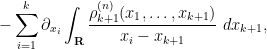
where the integral is interpreted in the principal value case. This system is an example of a BBGKY hierarchy.
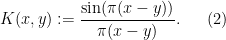
If one carefully rescales and takes limits (say at the energy level 


Informally, these equations show that the Dyson sine process 
where 
I recently set myself the exercise of deriving the identity (3) directly from the definition (1) of the Dyson sine process, without reference to GUE. This turns out to not be too difficult when done the right way (namely, by modifying the proof of Gaudin’s lemma), although it did take me an entire day of work before I realised this, and I could not find it in the literature (though I suspect that many people in the field have privately performed this exercise in the past). In any case, I am recording the computation here, largely because I really don’t want to have to do it again, but perhaps it will also be of interest to some readers.
This week I am at the American Institute of Mathematics, as an organiser on a workshop on the universality phenomenon in random matrices. There have been a number of interesting discussions so far in this workshop. Percy Deift, in a lecture on universality for invariant ensembles, gave some applications of what he only half-jokingly termed “the most important identity in mathematics”, namely the formula

whenever 


There are many ways to prove the identity. One is to observe first that when 


By rescaling, one obtains the variant identity

which essentially relates the characteristic polynomial of 


Thanks to this formula (and with a crucial insight of Alice Guionnet), I was able to solve a problem (on outliers for the circular law) that I had in the back of my mind for a few months, and initially posed to me by Larry Abbott; I hope to talk more about this in a future post.
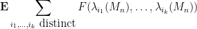
Today, though, I wish to talk about another piece of mathematics that emerged from an afternoon of free-form discussion that we managed to schedule within the AIM workshop. Specifically, we hammered out a heuristic model of the mesoscopic structure of the eigenvalues 

where 


At the macroscopic scale of 

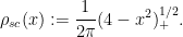
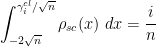
Indeed, if one defines the classical location 

![{[-2\sqrt{n}, 2\sqrt{n}]}](https://s0.wp.com/latex.php?latex=%7B%5B-2%5Csqrt%7Bn%7D%2C+2%5Csqrt%7Bn%7D%5D%7D&bg=ffffff&fg=000000&s=0&c=20201002)
then it is known that the random variable 


At the other extreme, at the microscopic scale of the mean eigenvalue spacing (which is comparable to 

Here, I wish to discuss the mesoscopic structure of the eigenvalues, in which one involves scales that are intermediate between the microscopic scale 


This is also the sum of the diagonal entries of a GUE matrix, and is thus normally distributed with a variance of 
Below the fold, I give a heuristic way to see this correlation, based on Taylor expansion of the convex Hamiltonian 

We can now turn attention to one of the centerpiece universality results in random matrix theory, namely the Wigner semi-circle law for Wigner matrices. Recall from previous notes that a Wigner Hermitian matrix ensemble is a random matrix ensemble 


In previous notes we saw that the operator norm of 


of
When 

Now we consider the behaviour of the ESD of a sequence of Hermitian matrix ensembles 


Remark 1 As usual, convergence almost surely implies convergence in probability, but not vice versa. In the special case of random probability measures, there is an even weaker notion of convergence, namely convergence in expectation, defined as follows. Given a random ESD
, defined via duality (the Riesz representation theorem) as
this probability measure can be viewed as the law of a random eigenvalue
drawn from a random matrix
converges the vague topology to
, thus
for all
.
In general, these notions of convergence are distinct from each other; but in practice, one often finds in random matrix theory that these notions are effectively equivalent to each other, thanks to the concentration of measure phenomenon.

Exercise 1 Let
- Show that
converges almost surely to
for all
.
- Show that
- Show that
converges to
We can now state the Wigner semi-circular law.
Theorem 1 (Semicircular law) Let
. Then the ESDs

A numerical example of this theorem in action can be seen at the MathWorld entry for this law.
The semi-circular law nicely complements the upper Bai-Yin theorem from Notes 3, which asserts that (in the case when the entries have finite fourth moment, at least), the matrices 
![{[-2,2]}](https://s0.wp.com/latex.php?latex=%7B%5B-2%2C2%5D%7D&bg=ffffff&fg=000000&s=0&c=20201002)

As will hopefully become clearer in the next set of notes, the semi-circular law is the noncommutative (or free probability) analogue of the central limit theorem, with the semi-circular distribution (1) taking on the role of the normal distribution. Of course, there is a striking difference between the two distributions, in that the former is compactly supported while the latter is merely subgaussian. One reason for this is that the concentration of measure phenomenon is more powerful in the case of ESDs of Wigner matrices than it is for averages of iid variables; compare the concentration of measure results in Notes 3 with those in Notes 1.
There are several ways to prove (or at least to heuristically justify) the semi-circular law. In this set of notes we shall focus on the two most popular methods, the moment method and the Stieltjes transform method, together with a third (heuristic) method based on Dyson Brownian motion (Notes 3b). In the next set of notes we shall also study the free probability method, and in the set of notes after that we use the determinantal processes method (although this method is initially only restricted to highly symmetric ensembles, such as GUE).
One theme in this course will be the central nature played by the gaussian random variables 
One way to exploit this algebraic structure is to continuously deform the variance 


At present, we have not completely specified what 

We will begin with one-dimensional Brownian motion, but it is a simple matter to extend the process to higher dimensions. In particular, we can define Brownian motion on vector spaces of matrices, such as the space of

Recent Comments