
As many readers may already know, my good friend and fellow mathematical blogger Tim Gowers, having wrapped up work on the Princeton Companion to Mathematics (which I believe is now in press), has begun another mathematical initiative, namely a “Tricks Wiki” to act as a repository for mathematical tricks and techniques. Tim has already started the ball rolling with several seed articles on his own blog, and asked me to also contribute some articles. (As I understand it, these articles will be migrated to the Wiki in a few months, once it is fully set up, and then they will evolve with edits and contributions by anyone who wishes to pitch in, in the spirit of Wikipedia; in particular, articles are not intended to be permanently authored or signed by any single contributor.)
So today I’d like to start by extracting some material from an old post of mine on “Amplification, arbitrage, and the tensor power trick” (as well as from some of the comments), and converting it to the Tricks Wiki format, while also taking the opportunity to add a few more examples.
Title: The tensor power trick
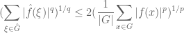
Quick description: If one wants to prove an inequality 


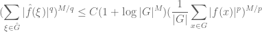
General discussion: This trick works best when using techniques which are “dimension-independent” (or depend only weakly (e.g. polynomially) on the ambient dimension M). On the other hand, the constant C is allowed to depend on other parameters than the dimension M. In particular, even if the eventual inequality 

It is of course essential that the problem “commutes” or otherwise “plays well” with the tensor power operation in order for the trick to be effective. In order for this to occur, one often has to phrase the problem in a sufficiently abstract setting, for instance generalising a one-dimensional problem to one in arbitrary dimensions.
Prerequisites: Advanced undergraduate analysis (real, complex, and Fourier). The user of the trick also has to be very comfortable with working in high-dimensional spaces such as 

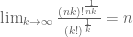
Example 1. (Convexity of 


As a first attempt to solve this problem, observe that 


But we can eliminate this loss of 2 by the tensor power trick. We pick a large integer 


From the Fubini-Tonelli theorem we see that

and similarly

If we thus apply our previous arguments with 


applying Fubini-Tonelli again we conclude that
Taking
Exercise. More generally, show that if 


whenever the right-hand side is finite, where 


Exercise. Use the previous exercise (and a clever choice of f, r, 
Example 2. (The maximum principle) This example is due to Landau. Let 


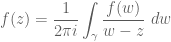
for 
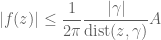
where 


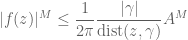
and on taking
Example 3. (New Strichartz estimates from old; this observation is due to Jon Bennet) Technically, this is not an application of the tensor power trick as we will not let the dimension go off to infinity, but it is certainly in a similar spirit.
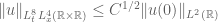
Strichartz estimates are an important tool in the theory of linear and nonlinear dispersive equations. Here is a typical such estimate: if 


for some absolute constant C. (In this case, the best value of C is known to equal 


Remark. A similar trick allows us to deduce “interaction” or “many-particle” Morawetz estimates for the Schrödinger equation from their more traditional “single-particle” counterparts; see for instance Chapter 3.5 of my book.
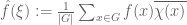
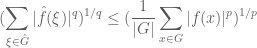
Example 4. (Hausdorff-Young inequality) Let G be a finite abelian group, and let 


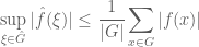
From the triangle inequality we have
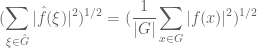
while from Plancherel’s theorem we have
By applying the Riesz-Thorin interpolation theorem, we can then conclude the Hausdorff-Young inequality
whenever 


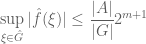
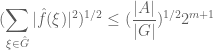
from which we establish a “restricted weak-type” version of Hausdorff-Young, namely
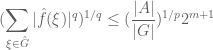
and thus
This inequality is restricted to those f whose non-zero magnitudes |f(x)| range inside a dyadic interval ![{}[2^m, 2^{m+1}]](https://s0.wp.com/latex.php?latex=%7B%7D%5B2%5Em%2C+2%5E%7Bm%2B1%7D%5D&bg=ffffff&fg=545454&s=0&c=20201002)


for general f. (There are of course an infinite number of dyadic scales 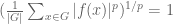


The estimate (3′) is off by a factor of
Taking 
Exercise. Establish Young’s inequality 


Exercise. Prove the Riesz-Thorin interpolation theorem (in the regime 
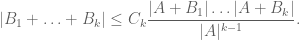
Example 5. (An example from additive combinatorics, due to Imre Ruzsa.) An important inequality of Plünnecke asserts, among other things, that for finite non-empty sets A, B of an additive group G, and any positive integer k, the iterated sumset 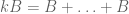

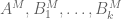
(This inequality, incidentally, is itself proven using a version of the tensor power trick, in conjunction with Hall’s marriage theorem, but never mind that here.) This inequality can be amplified to the more general inequality
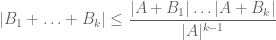
via the tensor power trick as follows. Applying (4) with 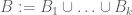
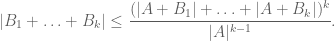
The right-hand side looks a bit too big, but we can resolve this problem with a Cartesian product trick (which can be viewed as a cousin of the tensor product trick). If we replace G with the larger group 


Optimising this in 

for some constant 

Example 6. (Cotlar-Knapp-Stein lemma) This example is not exactly a use of the tensor power trick, but is very much in the same spirit. Let 

for all i and some fixed A, then this is not enough to ensure that the sum 
for all i, then the very useful Cotlar-Knapp-Stein lemma asserts that 
Expanding the right-hand side out using the triangle inequality, we obtain

using (6) one soon ends up with a bound of 


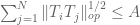
Now, one can estimate the operator norm 

or (using (5)) by

We take the geometric mean of these upper bounds to obtain

Summing this in 


Sending
Exercise. Show that the hypothesis of self-adjointness can be dropped if one replaces (6) with the two conditions
and

for all i.
Example 7. (Entropy estimates) Suppose that X is a random variable taking finitely many values. The Shannon entropy H(X) of this random variable is defined by the formula

where x runs over all possible values of X. For instance, if X is uniformly distributed over N values, then
If X is not uniformly distributed, then the formula is not quite as simple. However, the entropy formula (7) does simplify to the uniform distribution formula (8) after using the tensor power trick. More precisely, let 


which is of course consistent with the uniformly distributed case thanks to (8).
A key observation is that as 


One can use this “microstate” or “statistical mechanics” interpretation of entropy in conjunction with the tensor power trick to give short (heuristic) proofs of various fundamental entropy inequalities, such as the subadditivity inequality

whenever X, Y are discrete random variables which are not necessarily independent. Indeed, since 


taking
Exercise. Make the above arguments rigorous. (The final proof will be significantly longer than the standard proof of subadditivity based on Jensen’s inequality, but it may be clearer conceptually. One may also compare the arguments here with those in Example 1.)
Example 8. (Monotonicity of Perelman’s reduced volume) One of the key ingredients of Perelman’s proof of the Poincaré conjecture is a monotonicity formula for Ricci flows, that establishes that a certain geometric quantity, now known as the Perelman reduced volume, increases as time goes to negative infinity. Perelman gave both a rigorous proof and a heuristic proof of this formula. The heuristic proof is much shorter, and proceeds by first (formally) applying the Bishop-Gromov inequality for Ricci flat metrics (which shows that another geometric quantity – the Bishop-Gromov reduced volume, increases as the radius goes to infinity) not to the Ricci flow itself, but to a high-dimensional version of this Ricci flow formed by adjoining an M-dimensional sphere to the flow in a certain way, and then taking (formal) limits as
Example 9. (Riemann hypothesis for function fields) This example is much deeper than the previous ones, and I am not qualified to explain it in its entirety, but I can at least describe the one piece of this argument which uses the tensor power trick. For simplicity let us restrict attention to the Riemann hypothesis for curves C over a finite field 


where g is the genus of the curve, and 


As a corollary, we see that 

But because of the formula (10) and the functional equation, one can in fact deduce the Riemann hypothesis from the apparently weaker statement
where the implied constants can depend on the curve C, the prime p, and the genus g, but must be independent of the “dimension” M. Indeed, from (12) and (11) one can see that the largest magnitude of the
[This is of course only a small part of the story; the proof of (12) is by far the hardest part of the whole proof, and beyond the scope of this article.]
Further reading: The blog post “Amplification, arbitrage, and the tensor power trick” discusses the tensor product trick as an example of a more general “amplification trick”.

52 comments
Comments feed for this article
25 August, 2008 at 11:35 am
Mark Meckes
Here’s a very simple application of this trick, from this paper. The disadvantage is that it only proves a conditional result about an open problem.
Conjecture (the Gaussian Correlation Conjecture): Let denote the standard Gaussian probability measure on
  . Then for
  and
and  convex sets symmetric about the origin, we have
  .
.
Conditional theorem: it suffices to prove for some sequence
  such that
  .
.
Sketch of proof: For each , apply the known inequality to the
  -dimensional sets
  and
and  and take
  th roots.
The interest in such a conditional result is that it is also proved in the same paper that , which just falls short of being of use in connection with the conditional theorem.
25 August, 2008 at 3:44 pm
Anonymous
Cool post! One extraordinarily tiny correction: In your first example, in the two equations immediately following your first citation of Fubini-Tonelli, the rightmost should be
25 August, 2008 at 5:14 pm
Terence Tao
Dear Mark: Thanks for the example! It does seem that problems involving gaussians tend to be particularly amenable to the tensor power trick.
Dear Anonymous: thanks for the correction!
25 August, 2008 at 8:04 pm
Pete L. Clark
Dear Prof. Tao,
I’m surprised that you didn’t mention (here) the use of this sort of trick in Z. Dvir’s bounds for Kakeya sets over finite fields. In
Click to access Dvir08b.pdf
he uses it to deduce Corollary 1.2 from Theorem 1.1. Admittedly it does not quite fit your model, because here the constant _does_ scale with the
dimension. (Ironically, the improvements given by Alon and yourself circumvent this argument.) Prof. Laba in her blog entry
describes this as a “standard product set argument”, so I gather there are other Kakeya-type examples.
25 August, 2008 at 10:13 pm
Suresh
Another application of the tensor trick is in proving that certain NP-hard problems are even hard to approximate well. A standard direct application of this is to prove that CLIQUE cannot be approximated to any constant factor (by taking graph products repeatedly).
26 August, 2008 at 12:43 am
gowers
Dear Terry,
Many thanks for doing this — it will be a superb article for the site. Can I just take the chance to say two things? First, although we don’t have a definite date yet, we are hoping that it will be up and running, in some form at least, by the end of September, so a little sooner than you suggest. The other thing is to anyone who might be reading this: if you can think of a class of problems that you once found difficult and now find easy, at whatever level (anything from high school to cutting-edge research), and if you can explain clearly what it is that you now understand that you didn’t understand before, then please consider writing an article about it for the site. We’re eventually aiming for something very comprehensive, but in the initial stages we’d just like to get quickly to a large selection of interesting articles.
Tim
26 August, 2008 at 7:37 am
Felipe Voloch
Another application of this trick is to show that, for a norm on a field, the condition that the set of integers is bounded (non-archimedian property) implies the condition that the strong triangle inequality (ultrametric property) holds. Apply the usual triangle inequality to the binomial expansion of (x+y)^n and take n-th roots. The converse implication also holds and it’s easier.
26 August, 2008 at 7:47 am
Izabella Laba
Pete L. Clark:
There’s a very similar argument in this paper by Katz and Tao (see the end of the proof of Lemma 2.1).
26 August, 2008 at 10:02 am
Anonymous
Hello Professor Tao,
Thanks for posting that. I thought of another example, which though not really analysis seems somewhat relevant: If G is a group, then the dimension of any irreducible representation of G divides the index (G:C) where C is the center (I believe this is due to Tate). Let V be an irreducible representation of degree and take the tensor power
  , which is an irreducible representation for
  . The subgroup
  consisting of elements
  such that each
  and
and  acts trivially on
  . This means that we have an irreducible representation of
  on
on  , whose dimension is
  . Then since the dimension of an irreducible representation of a group divides the order of that group, and since the order of
  is
is  , we have:
  . Here
  is the order of
  ,
,  is the order of
  . Choosing
  very large, we get
  .
.
26 August, 2008 at 10:52 am
Gergely Harcos
One can learn from these posts, thanks! Two small suggestions: and
and  in the preceding Exercise. In (3) we have
  in place of
  .
.
In the Exercise about Hölder’s inequality I would include the additional hint that one can take
26 August, 2008 at 2:17 pm
Singularitarian
Wow, what a great blog where you have talented mathematicians posting insightful comments. Learning math is a lot easier than it used to be. (But it is still hard.)
27 August, 2008 at 2:08 am
Gergely Harcos
Actually there are two displays numbered (3). I meant the display right after (2) in Example 4.
27 August, 2008 at 5:02 am
Anonymous
I apologize for making a mistake in the proof of the result of Tate on group representations I posted above. The subgroup acts trivially
  because
  consists of a m-tuple of elements of the center
  of
of  . By Schur’s lemma, each of these elements is a homothety. This implies the statement. (Otherwise the theorem would work for arbitrary abelian normal subgroups.)
27 August, 2008 at 9:40 am
Terence Tao
Thanks for the corrections and the many further examples! I can add one more from my own blog: the Mahler conjecture for convex bodies tensorises in much the same way as Mark’s example above.
27 August, 2008 at 7:32 pm
Richard Borcherds.
Example 9 can be extended a bit: Deligne used this idea in his proof of the Riemann
hypothesis in higher dimensions. Roughly speaking, he shows that any zero z of the Weil zeta function must be within a distance 1/2 of the critical line. Applying this to the n’th power of the variety shows that nz must also be within a distance 1/2 of some critical line, so z must be within a distance 1/2n of some critical line for any n.
Exercise: find a good way to take products of Spec Z with itself. A good solution will prove the Riemann hypothesis for the Riemann zeta function.
27 August, 2008 at 10:45 pm
A wiki for math tricks! « Entertaining Research
[…] wiki for math tricks! Terence Tao brings these glad tidings with his latest post: As many readers may already know, my good friend and fellow mathematical blogger Tim Gowers, […]
28 August, 2008 at 1:59 am
Emmanuel Kowalski
Deligne’s argument was “helped” by the fact that given a polynomial zeta function with roots , there is another one with roots
  , whose analytic properties could be established. For the Riemann zeta function, getting to additive normalization, a directly similar reasoning would need to know that there is a “natural” zeta function with zeros
  , where
  and
and  run over zeros of
  . I think some people have looked a bit, and such functions do not seem to be so nice (for instance, they do not seem to be automorphic
  -functions).
28 August, 2008 at 2:55 am
Frank Morgan
Thanks to Gergely Harcos for additional hint for exercise about Hölder’s inequality.
28 August, 2008 at 11:14 am
Gergely Harcos
After the comments by Professors Borcherds and Kowalski I am tempted to remark that the Langlands Program envisions a proof of the Ramanujan-Selberg conjectures also by a tensor power trick. Namely, if is a Langlands parameter at a “nice prime” p of some automorphic form f then we expect, for each positive integer n, that there is some sort of “n-th power of f”, an automorphic form which has
  as a Langlands parameter at p. A general bound for Langlands parameters then would tell us that
  , hence in fact
  .
.
29 August, 2008 at 11:03 am
John Baez
I like the idea of a “Tricks Wiki”, but surely it would be more fun to call it a “Tricky Wiki”.
29 August, 2008 at 5:16 pm
Chris
Speaking of clever or cute names, how about TiddlyWiki.
(There is more of interest here than just the name!)
5 September, 2008 at 3:31 pm
Jose Brox
(I apologize for repeating this comment at the two blogs)
I see I arrived a bit late to the party. Nevertheless I hope this comment
gets read somehow :D
· First thing I thought about the subject: we NEED to get organized! In particular, we need to open a forum about the Tricki: the planification and organization of such a feat can’t be done from the zero-level, we must keep adding layers of data and information distribution until we arrive to the Wiki, and it seems to me that the first step should be a forum (blogs were the 0-step).
· About the difficult and fascinating subject of naming and identifying every trick (btw, this should be not a thread, but a whole subforum on the forum!):
a) I suggest we “impose” the official name, by being the de facto most authoritative source for math tricks (as it happens with OEIS or Wikipedia). Once we have launched the project and having such skilled, expert, famous people on it, authority will follow fast. People will tend to use the names we give to the tricks just because the rest of the people will want to look at them at our Wiki (here, when I say “we” and “our” I refer to everyone who wants to collaborate, of course!)
b) The name should be composed of (at least) three components:
1) An informal, catchy name.
This would be the best known name for the trick, and would methaphorically refer to its use or main characteristics, or to any circumstances around it or its first apparition, like theorems tend to be named “lately” (hairy ball theorem, sandwich theorem, rising sun lemma, egregius theorem, etc).
The word “TRICK” (or any other to be decide) should be the last name, just to let people know what we are talking about.
An invented example: The “1-is-not-so-trivial” trick -> In your main FORMULA [specialized term to be defined within the WIKI], substitute 1 for any fancy SUBFORMULA that does equal to 1, like sin^2(x)+cos^2(x), or partitions of unity, and REARRANGE the main formula (i.e. separate in “components”, simplify, glue, etc).
2) A technical name within an a priori specified naming rule system (to be defined yet) that already implies some categorization, something like the naming of new biological species. For example: FORMULA SUBSTITUTING+ (where Formula refers to the fact that the trick is about formulas, Substituting refers to the obvious fact, and the “+” means that the substitution actually gets more complex, and not less (-)).
Another invented categorization family name could be
Equation DifferentiatingN (take your equation and differentiate it N times)
3) A serial number. Just to catalogue the trick and make internal database work with it (but also to have it uniquely identified!)
c) To solve the search problem, a multitag system looks like the most reasonable system to me, but the selection of the tags is critical. I think we should have two kinds of tag:
predetermined distinguished tags, and configurably non-distinguished tags. The first ones would be created with the project (always subject to suggestions and changes) and would be things like:
WHERE (in which branchs of math)
IN (in which type of structures)
FROM (hypothesis and elements you need to have for the trick to make sense; i.e. the trick starting point)
TO (the generic result you accomplish by applying the trick)
WITH (”the how”, technical terms that describe key parts of the process)
NAME (informal name)
CATEGORY (formal name),
SN (serial number)
AUTHOR (the creator or best-known user of the trick, if it’s known)
REFERENCE (well-kown book, paper or source where it’s used in an important manner)
USES (well-known uses of this trick, theorems where it is important, etc)
The non-distinguished tags would all fall to the same category OTHERS, as a list, just like the tags in YouTube.
Not all the tags need to be filled, and some can be multivalued.
An example:
SN 0000
NAME “The connection trick”
CATEGORY Set Identificating Connected
WHERE Topology, Algebraic Topology
IN Topological spaces, Manifolds
FROM Connected set, subset
TO Subset is Whole Set
WITH Connected Sets Open-Closed Characterization
USES
OTHER Standard, Basic
Did you know what trick it was? The informal description (which I think it should be the first thing you get after the tags) would be “In a connected set C there are no subsets that are open and closed at the same time, other than the empty set and C. Therefore, if you want to prove that your subset D of your connected set S is in fact the whole S, just prove that D is open, closed, and non-empty”
·Other basic tricks I thought of just know (please forgive their triviality, I’m just a math student yet):
* Smart application of Hölder inequality
* Partitions of unity
* Linearization in the axioms of non-associative algebras
* Zorn’s Lemma and, similarly, the Ascending Chain Condition and Maximal Condition for noetherian modules
* If in a Normed Space you want to prove that x is 0, just prove that its norm is 0
* If you want to observe the ideals that contain I, then study A/I. If you want to study the ideals contained in the prime P, study the localization A_P.
* If you are working in a bound that involves exp(x) maybe you just need to work with (1+x). In general, if you are working in a bound that involves an analytic function, it may suffice to work with the first n terms of its Taylor Series (where n=0,1,…,5).
Well, I’ll adore to give more ideas and to get really involved with this great project, but we definitely need a forum! (If it isn’t implemented yet!). The other way all this effort will eventually come to waste…
Regards!
Jose Brox
16 September, 2008 at 6:39 am
Max Rabkin
Can you please turn off Snap Previews on your blog? I’d love to read it more often, but Snap Previews turn me off.
30 September, 2008 at 11:08 am
John Mangual
I agree. Snap Previews have the merit of being both useful and annoying. :-)
I really like the idea of “trickopedia.” There are many cases when the ideas in the proof are more useful to learn than the statement being proved. For example, if I learn about Ostrowski’s theorem in a book on p-adic numbers, the only place I learn to think abstractly about valuations is in the proof itself. Incidentally, the proof in Section 1.2 of Neal Koblitz’ book on p-adic numbers uses something like the “tensor-power trick”. In any case, I think such a site would have helped me in my studies as an undergraduate.
15 October, 2008 at 9:52 am
The forthcoming launch of the Tricki « Gowers’s Weblog
[…] See some of my recent blog posts for examples of articles written in this format. See also this article by Terence Tao, and this one by Emmanuel […]
24 October, 2008 at 3:55 pm
Distinguished Lecture Series II: Elias Stein, “The Cauchy integral in C^n” « What’s new
[…] or decay exponentially fast in . Applying the Cotlar-Stein lemma (which I discussed in this earlier blog post) one obtains the […]
10 January, 2009 at 4:28 pm
245B, notes 3: L^p spaces « What’s new
[…] Remark 4. For a different proof of this inequality (based on the tensor power trick), see Example 1 of this blog post of mine. […]
5 March, 2009 at 7:21 pm
Anonymous
it so difficult to understand……………………………………………………………………………
26 March, 2009 at 7:20 pm
While I’m linking… « Feed The Bears
[…] A further post on the tensor power trick. This gives more details an examples than the first post on how to use the tensor power trick. […]
30 March, 2009 at 8:58 am
245C, Notes 1: Interpolation of L^p spaces « What’s new
[…] is off by a constant factor by what we want. But one can eliminate this constant by using the tensor power trick. Indeed, if one replaces with a Cartesian power (with the product -algebra and product measure […]
6 April, 2009 at 2:59 pm
254C, Notes 2: The Fourier transform « What’s new
[…] asserts that the Fourier transform commutes with tensor products. (Because of this fact, the tensor power trick is often available when proving results about the Fourier transform on general groups.) Exercise […]
25 May, 2009 at 4:52 am
orr
Hello,
In example 2, in the denominator, w and z should be swapped (otherwise integrate in the clockwise direction). [Corrected, thanks – T.]
12 October, 2009 at 8:32 am
Divisibility theorems for group representations « Delta Epsilons
[…] proof (due to Tate) is an amusing application of the tensor power trick; one fixes an irreducible , and considers the representation of the direct product , which is […]
10 February, 2011 at 3:59 am
A new way of proving sumset estimates « Gowers's Weblog
[…] of which is a trivially sufficient condition for the inequality to hold in this case); using the tensor product trick and the construction of Plünnecke graphs that approximately have certain magnification ratios, […]
20 December, 2011 at 12:41 pm
The spectral theorem and its converses for unbounded symmetric operators « What’s new
[…] (v) Show that for all . Improve the to . (Hint: to get this improvement, use the identity and the tensor power trick.) […]
20 December, 2011 at 12:50 pm
The spectral theorem and its converses for unbounded symmetric operators | t1u
[…] (v) Show that for all . Improve the to . (Hint: to get this improvement, use the identity and the tensor power trick.) […]
31 August, 2012 at 5:03 pm
The Lang-Weil bound « What’s new
[…] For technical reasons, we only prove these bounds directly when is a perfect square; the general case then follows by using the explicit formula for as a function of and the tensor power trick, as explained in this previous post. […]
7 December, 2012 at 1:06 am
Ofir Gorodetsky
Hello Prof. Tao, :
:

 ‘th root, the AM-GM follows by the following limit:
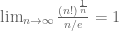 . Alternatively, one can say that
  is the largest binomial coefficient, hence
  , and after taking the
  ‘th power and
  , we’re done again.
Thank your for this beautiful post. I can share another example of this method – Harald Bohr’s proof of the arithmetic-geometric mean (in a paper named “The Arithmetic and Geometric Means”). It goes as follows:
By expanding, one can show that for any
Taking the
One doesn’t need Stirling’s approximation, merely the simple limit
12 June, 2013 at 2:13 pm
Estimation of the Type I and Type II sums | What's new
[…] that (this trick to “magically” delete the error is a canonical example of the tensor power trick), and the bound (15) then follows from […]
2 May, 2014 at 5:54 pm
The Bombieri-Stepanov proof of the Hasse-Weil bound | What's new
[…] upper bound to a matching lower bound, and if one then uses the trace formula (1) (and the “tensor power trick” of sending to infinity to control the weights ) one can then recover the full Hasse-Weil […]
13 May, 2014 at 9:36 pm
Dwork’s proof of rationality of the zeta function over finite fields | What's new
[…] we can prove the ultra-triangle inequality via the tensor power trick. If , then from (4) we […]
16 May, 2018 at 4:19 pm
Convex sets have many differences | George Shakan
[…] This would imply Conjecture (Convex) and Conjecture 1 for . The goal of the rest of this post is to prove the current state of the art progress due to Shkredov and Schoen. The proof of Theorem 1 is simple enough that we compute the constant (though one can remove it using the tensor power trick). […]
19 May, 2018 at 2:44 pm
Anonymous
In Example 4, does the trick work for the setting of Euclidean spaces instead of finite abelian groups?
20 May, 2018 at 1:58 pm
Terence Tao
With a little bit of effort, yes. Alternatively, once one has the Hausdorff-Young inequality for finite abelian groups, one can deduce the corresponding inequality on Euclidean spaces, basically by approximating the Euclidean Fourier transform by a discrete Fourier transform (assuming to begin with that the function belongs for instance to the Schwartz class, and removing this hypothesis with a limiting argument later).
2 May, 2020 at 11:10 am
247B, Notes 3: pseudodifferential operators | What's new
[…] the way to by iterating the method (this is an instance of a neat trick in analysis, namely the tensor power trick). For any integer that is a power of two, we see from iterating the method […]
9 June, 2020 at 2:09 pm
Anonymous
I have seen tensor product of (multi)linear maps. Is it just a convenient notion or is there an algebraic setting for the tensor product of arbitrary maps as in this post?
18 November, 2022 at 4:09 am
gdallara
Dear Tao,
concerning Riesz-Thorin theorem, are you claiming that one can recover the full statement, without the restriction ? It seems to me that one needs to know that
  , and I am only able to prove it if
  . But that could be a limit of my argument, of course…
19 November, 2022 at 3:51 am
Gian Maria D
ps. I just realized that the tensor power trick argument I had in mind does not distinguish the real from the complex case, and over the reals one one does not have log-convexity of operator norms on the upper triangle .
.
20 November, 2022 at 1:54 pm
Terence Tao
There are two proofs of this identity, one that works for and one that does not require this restriction. See (2.11) (and footnote 4) in this recent paper of Ben Krause, Marius Mirek and myself.
23 November, 2022 at 7:50 am
Gian Maria D
Thanks! If I understand correctly, the linked paper indeed observes that one has the needed multiplicativity of the operator norm under tensoring when either or the kernel is nonnegative.
Nevertheless, the log-convexity bound
does not hold for general -linear operators in the range
  (Riesz 1927 paper shows that a 45 degrees rotation in
  is a counterexample).
Hence, my suspect is that there cannot be a real-variable argument of Riesz-Thorin in complete generality. Does this make sense?
25 November, 2022 at 3:30 pm
Terence Tao
Hmm, I did not appreciate this subtlety before, that there are cases of Riesz-Thorin that lie outside of the scope of the tensor product trick (at least as naively applied). Will modify the text appropriately.
26 November, 2022 at 6:34 am
Gian Maria D
It seems indeed to be pretty subtle: given a real operator, one may complexify it, apply the complex Riesz-Thorin theorem, and recover an “almost log-convexity bound” in the real case:
where the implicit constant is absolute. If it were possible to apply the tensor power trick in the real case, one would expect this absolute constant to go away. But again, the rotation example shows that this cannot be done.
The moral is that one should use the fact that the ground field is in the proof of Riesz-Thorin.