Let  and
and  be two random variables taking values in the same (discrete) range
  , and let
  be some subset of , which we think of as the set of “bad” outcomes for either or . If and have the same probability distribution, then clearly

In particular, if it is rare for to lie in , then it is also rare for to lie in .
If and do not have exactly the same probability distribution, but their probability distributions are close to each other in some sense, then we can expect to have an approximate version of the above statement. For instance, from the definition of the total variation distance  between two random variables (or more precisely, the total variation distance between the probability distributions of two random variables), we see that

for any  . In particular, if it is rare for to lie in , and
  are close in total variation, then it is also rare for to lie in .
A basic inequality in information theory is Pinsker’s inequality

where the Kullback-Leibler divergence  is defined by the formula

(See this previous blog post for a proof of this inequality.) A standard application of Jensen’s inequality reveals that is non-negative (Gibbs’ inequality), and vanishes if and only if , have the same distribution; thus one can think of as a measure of how close the distributions of and are to each other, although one should caution that this is not a symmetric notion of distance, as  in general. Inserting Pinsker’s inequality into (1), we see for instance that

Thus, if is close to in the Kullback-Leibler sense, and it is rare for to lie in , then it is rare for to lie in as well.
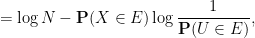
We can specialise this inequality to the case when a uniform random variable  on a finite range of some cardinality
  , in which case the Kullback-Leibler divergence
  simplifies to

where
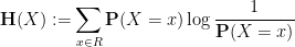
is the Shannon entropy of . Again, a routine application of Jensen’s inequality shows that  , with equality if and only if is uniformly distributed on . The above inequality then becomes

Thus, if is a small fraction of (so that it is rare for to lie in ), and the entropy of is very close to the maximum possible value of  , then it is rare for to lie in also.
The inequality (2) is only useful when the entropy  is close to in the sense that
  , otherwise the bound is worse than the trivial bound of
  . In my recent paper on the Chowla and Elliott conjectures, I ended up using a variant of (2) which was still non-trivial when the entropy was allowed to be smaller than
  . More precisely, I used the following simple inequality, which is implicit in the arguments of that paper but which I would like to make more explicit in this post:
Lemma 1 (Pinsker-type inequality) Let be a random variable taking values in a finite range of cardinality , let be a uniformly distributed random variable in , and let be a subset of . Then

Proof: Consider the conditional entropy  . On the one hand, we have


by Jensen’s inequality. On the other hand, one has


where we have again used Jensen’s inequality. Putting the two inequalities together, we obtain the claim. 
Remark 2 As noted in comments, this inequality can be viewed as a special case of the more general inequality

for arbitrary random variables taking values in the same discrete range , which follows from the data processing inequality

for arbitrary functions  , applied to the indicator function
  . Indeed one has
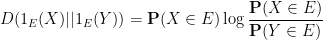

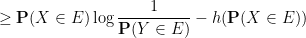

where  is the entropy function.
Thus, for instance, if one has

and

for some  much larger than
  (so that
  ), then

More informally: if the entropy of is somewhat close to the maximum possible value of , and it is exponentially rare for a uniform variable to lie in , then it is still somewhat rare for to lie in . The estimate given is close to sharp in this regime, as can be seen by calculating the entropy of a random variable which is uniformly distributed inside a small set with some probability  and uniformly distributed outside of with probability
  , for some parameter
  .
.
It turns out that the above lemma combines well with concentration of measure estimates; in my paper, I used one of the simplest such estimates, namely Hoeffding’s inequality, but there are of course many other estimates of this type (see e.g. this previous blog post for some others). Roughly speaking, concentration of measure inequalities allow one to make approximations such as

with exponentially high probability, where is a uniform distribution and  is some reasonable function of . Combining this with the above lemma, we can then obtain approximations of the form

with somewhat high probability, if the entropy of is somewhat close to maximum. This observation, combined with an “entropy decrement argument” that allowed one to arrive at a situation in which the relevant random variable did have a near-maximum entropy, is the key new idea in my recent paper; for instance, one can use the approximation (3) to obtain an approximation of the form


for “most” choices of  and a suitable choice of
  (with the latter being provided by the entropy decrement argument). The left-hand side is tied to Chowla-type sums such as
  through the multiplicativity of
  , while the right-hand side, being a linear correlation involving two parameters
  rather than just one, has “finite complexity” and can be treated by existing techniques such as the Hardy-Littlewood circle method. One could hope that one could similarly use approximations such as (3) in other problems in analytic number theory or combinatorics.


14 comments
Comments feed for this article
20 September, 2015 at 11:23 am
Anonymous
Dear Prof. Tao,
There is a simple exponential version of Pinsker’s inequality that almost gives what you want, even without the assumption that one of the RV’s is uniform:
\delta(X,Y) \le 1 – (1/2).exp(-KL(X,Y))
(This is proved for instance in Tsybakov’s book “Introduction to Nonparametric Estimation” (eq. 2.25).) Unfortunately this only gives constant bounds, instead of o(1), in your setting.
20 September, 2015 at 11:53 am
Yihong
A side remark on Lemma 1: (2) also follows from the “data processing” inequality in information theory, namely, , for any function
  . Taking
  implies (2). Furthermore, instead of deterministic
  , one can replace
  by any Markov kernel. Lemma 1 is useful in information-theoretic treatment of large deviation. For example, taking
  and
and  with iid components and
  shows that the large deviation exponent cannot exceed something, an idea due to Csiszar, see, e.g., http://www.emis.de/journals/em/docs/boletim/vol374/v37-4-a2-2006.pdf
[Nice! I’ve added this alternate argument to the main post. -T.]
21 September, 2015 at 2:34 am
K
What was the motivation from data processing for their inequality?
20 September, 2015 at 5:29 pm
David Roberts
The Remark 2 box has a broken equation. Also, at one point, shortly after KL-divergence is defined, you’ve got D_{KL}(X|Y).
[Corrected, thanks – T.]
21 September, 2015 at 12:13 pm
John Mangual
Can the prime number theorem as a kind of concentration of measure phenomenon? E.g. we can show Möbius valued coin-flips are not biased.
I don’t know how to formulate this precisely. Even the law of large numbers itself is fraught with difficult philosophical questions like “what is a typical infinite random sequence of coin flips?”
All proofs of PNT I have seen so far, ultimately lose their combinatorial flavor and either become delicate (but common) maneuvers of the zeta function with contour integrals or, equally challenging estimates about (starting with Bertrand’s postulate).
In either case you can’t just conclude “gee that is the max-ent distribution” but you have to prove that entropy is increasing – this is hard. I find many expositions of PNT start off great, but wind up sweeping important sources of complexity under the rug. Sadly, I have not said very much.
24 September, 2015 at 11:55 pm
Jesper
If you use the definition of total variation distance given on Wikipedia, then the constant in Pinsker’s inequality can be improved to 1/2. A constant of 2 is only needed if one defines the total variation distance to be the L_1 distance (in the Wikipedia definition, the total variation distance is half the L_1 distance).
[Corrected, thanks – T.]
3 October, 2015 at 4:26 am
Anonymous
Since there are several kinds of entropies (e.g. Gibbs, Shannon, Perelman), is there some unifying definition of entropy for general (for both stochastic or deterministic) dynamical systems ?
4 October, 2015 at 1:32 am
PerryZhao
Reblogged this on 木秀于林.
14 October, 2015 at 5:34 am
Bowen
Reblogged this on Statistics & ML Hack.
17 October, 2015 at 9:37 am
Steven Heilman
Is it possible to re-interpret your Pinsker inequalities using the Ricci curvature of the graph G_n,H discussed in the previous post? It is known (Theorem 1.10, http://arxiv.org/pdf/1509.07160v1.pdf) that if a graph has “positive Ricci curvature,” then the graph satisfies a Pinsker inequality. (See also: http://cedricvillani.org/wp-content/uploads/2012/07/031.BV-CKP.pdf). Checking for “positive Ricci curvature” typically amounts to showing that the graph has many short cycles, and it seems that the graph G_n,H has many short cycles. Unfortunately, maybe each of you has a different definition of a Pinsker inequality, so it may be difficult to connect these topics.
17 October, 2015 at 10:23 am
Terence Tao
As far as I can tell, these are unrelated uses of graphs. In the papers you cite, the Pinsker inequality is generalised by placing a graph metric on the underlying sample space that the probability measures are supported on, sand then replacing total variation norm with Wasserstein distance. With the random graphs G_n, the graphs are not used as sample spaces, but instead each outcome in the sample space is associated to one such graph. The metric geometry of these graphs is somewhat related to their expansion properties (e.g. expanders tend to have very small diameter, and the spectral gap property of expanders is closely tied to the existence of a Poincare inequality), but it’s unclear to me how to take advantage of this if one wishes to establish expansion of these graphs.
28 October, 2015 at 12:28 pm
Grisou
Hello,
Very interesting.
Is there any similar result for continuous random variables X and Y ?
5 March, 2017 at 10:39 am
Furstenberg limits of the Liouville function | What's new
[…] some . Using the Pinsker-type inequality from this previous blog post, we conclude the lower […]
4 November, 2018 at 8:45 am
Tao’s Proof of (logarithmically averaged) Chowla’s conjecture for two point correlations | I Can't Believe It's Not Random!
[…] Proof: This is Lemma 1 in this post of Tao. […]