Online reading seminar for Zhang’s “bounded gaps between primes”

4 June, 2013 in math.NT, polymath | Tags: polymath8, Yitang Zhang

In a recent paper, Yitang Zhang has proven the following theorem:

Theorem 1 (Bounded gaps between primes) There exists a natural number ${H}$ such that there are infinitely many pairs of distinct primes ${p,q}$ with ${|p-q| \leq H}$ .

Zhang obtained the explicit value of ${70,000,000}$ for ${H}$ . A polymath project has been proposed to lower this value and also to improve the understanding of Zhang’s results; as of this time of writing, the current “world record” is ${H = 4,802,222}$ (and the link given should stay updated with the most recent progress.

Zhang’s argument naturally divides into three steps, which we describe in reverse order. The last step, which is the most elementary, is to deduce the above theorem from the following weak version of the Dickson-Hardy-Littlewood (DHL) conjecture for some ${k_0}$ :

Theorem 2 ( ${DHL[k_0,2]}$ ) Let ${{\mathcal H}}$ be an admissible ${k_0}$ -tuple, that is to say a tuple of ${k_0}$ distinct integers which avoids at least one residue class mod ${p}$ for every prime ${p}$ . Then there are infinitely many translates of ${{\mathcal H}}$ that contain at least two primes.

Zhang obtained ${DHL[k_0,2]}$ for ${k_0 = 3,500,000}$ . The current best value of ${k_0}$ is ${341,640}$ , as discussed in this previous blog post. To get from ${DHL[k_0,2]}$ to Theorem 1, one has to exhibit an admissible ${k_0}$ -tuple of diameter at most ${H}$ . For instance, with ${k_0 = 341,640}$ , the narrowest admissible ${k_0}$ -tuple that we can construct has diameter ${4,802,222}$ , which explains the current world record. There is an active discussion on trying to improve the constructions of admissible tuples at this blog post; it is conceivable that some combination of computer search and clever combinatorial constructions could obtain slightly better values of ${H}$ for a given value of ${k_0}$ . The relationship between ${H}$ and ${k_0}$ is approximately of the form ${H \approx k_0 \log k_0}$ (and a classical estimate of Montgomery and Vaughan tells us that we cannot make ${H}$ much narrower than ${\frac{1}{2} k_0 \log k_0}$ , see this previous post for some related discussion).

The second step in Zhang’s argument, which is somewhat less elementary (relying primarily on the sieve theory of Goldston, Yildirim, Pintz, and Motohashi), is to deduce ${DHL[k_0,2]}$ from a certain conjecture ${MPZ[\varpi,\delta]}$ for some ${\varpi,\delta > 0}$ . Here is one formulation of the conjecture, more or less as (implicitly) stated in Zhang’s paper:

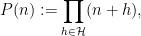
Conjecture 3 ( ${MPZ[\varpi,\delta]}$ ) Let ${{\mathcal H}}$ be an admissible tuple, let ${h_i}$ be an element of ${{\mathcal H}}$ , let ${x}$ be a large parameter, and define

$\displaystyle D := x^{1/4+\varpi},$

$\displaystyle {\mathcal P} := \prod_{p: p < x^{\delta}} p,$

$\displaystyle P(n) := \prod_{h \in {\mathcal H}} (n+h),$

$\displaystyle C_i(d) := \{ c \in {\bf Z}/d{\bf Z}: (c,d) = 1; P(c-h_i) = 0 \hbox{ mod } d \}$

for any natural number ${d}$ , and

$\displaystyle \Delta(\gamma;d,c) = \sum_{x \leq n \leq 2x: n = c \hbox{ mod } d} \gamma(n) - \frac{1}{\varphi(d)} \sum_{x \leq n \leq 2x: (n,d) = 1} \gamma(n)$

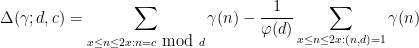
for any function ${\gamma: {\bf N} \rightarrow {\bf C}}$ . Let ${\theta(n)}$ equal ${\log p}$ when ${n}$ is a prime ${p}$ , and ${\theta(n)=0}$ otherwise. Then one has

$\displaystyle \sum_{d < D^2; d|{\mathcal P}} \sum_{c \in C_i(d)} |\Delta(\theta; d, c )| \ll x \log^{-A} x$

for any fixed ${A > 0}$ .

Note that this is slightly different from the formulation of ${MPZ[\varpi]}$ in the previous post; I have reverted to Zhang’s formulation here as the primary purpose of this post is to read through Zhang’s paper. However, I have distinguished two separate parameters here ${\varpi,\delta}$ instead of one, as it appears that there is some room to optimise by making these two parameters different.

In the previous post, I described how one can deduce ${DHL[k_0,2]}$ from ${MPZ[\varpi,\delta]}$ . Ignoring an exponentially small error ${\kappa}$ , it turns out that one can deduce ${DHL[k_0,2]}$ from ${MPZ[\varpi,\delta]}$ whenever one can find a smooth function ${g: [0,1] \rightarrow {\bf R}}$ vanishing to order at least ${k_0}$ at ${1}$ such that

$\displaystyle k_0 \int_0^1 g^{(k_0-1)}(x)^2 \frac{x^{k_0-2}}{(k_0-2)!}\ dx > \frac{4}{1+4\varpi} \int_0^1 g^{(k_0)}(x)^2 \frac{x^{k_0-1}}{(k_0-1)!}\ dx.$

By selecting ${g(x) := \frac{1}{(k_0+l_0)!} (1-x)^{k_0+l_0}}$ for a real parameter ${l_0>0}$ to optimise over, and ignoring the technical ${\kappa}$ term alluded to previously (which is the only quantity here that depends on ${\delta}$ ), this gives ${DHL[k_0,2]}$ from ${MPZ[\varpi,\delta]}$ whenever

$\displaystyle k_0 > (\sqrt{1+4\varpi} - 1)^{-2} \ \ \ \ \ (1)$

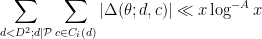
It may be possible to do better than this by choosing smarter choices for ${g}$ , or performing some sort of numerical calculus of variations or spectral theory; people interested in this topic are invited to discuss it in the previous post.

The final, and deepest, part of Zhang’s work is the following theorem (Theorem 2 from Zhang’s paper, whose proof occupies Sections 6-13 of that paper, and is about 32 pages long):

Theorem 4 (Zhang) ${MPZ[\varpi,\varpi]}$ is true for all ${0 < \varpi \leq \frac{1}{1168}}$ .

The significance of the fraction ${1/1168}$ is that Zhang’s argument proceeds for a general choice of ${\varpi > 0}$ , but ultimately the argument only closes if one has

$\displaystyle \frac{31}{32} + 36 \varpi \leq 1 - \frac{\varpi}{2}$

(see page 53 of Zhang) which is equivalent to ${\varpi \leq 1/1168}$ . Plugging in this choice of ${\varpi}$ into (1) then gives ${DHL[k_0,2]}$ with ${k_0 = 341,640}$ as stated previously.

Improving the value of ${\varpi}$ in Theorem 4 would lead to improvements in ${k_0}$ and then ${H}$ as discussed above. The purpose of this reading seminar is then twofold:

Going through Zhang’s argument in order to improve the value of ${\varpi}$ (perhaps by decreasing ${\delta}$ ); and
Gaining a more holistic understanding of Zhang’s argument (and perhaps to find some more “global” improvements to that argument), as well as related arguments such as the prior work of Bombieri, Fouvry, Friedlander, and Iwaniec that Zhang’s work is based on.

In addition to reading through Zhang’s paper, the following material is likely to be relevant:

A recent blog post of Emmanuel Kowalski on the technical details of Zhang’s argument.
Scanned notes from a talk related to the above blog post.
A recent expository note by Fouvry, Kowalski, and Michel on a Friedlander-Iwaniec character sum relevant to this argument.
This 1981 paper of Fouvry and Iwaniec which is the first result in the literature which is roughly of the type ${MPZ[\varpi,\delta]}$ . (This paper seems to give a related result for ${\varpi=1/42}$ and ${\delta = 1/883}$ , if I read it correctly; I don’t yet understand what prevents this result or modifications thereof from being used in place of Theorem 4.)

I envisage a loose, unstructured format for the reading seminar. In the comments below, I am going to post my own impressions, questions, and remarks as I start going through the material, and I encourage other participants to do the same. The most obvious thing to do is to go through Zhang’s Sections 6-13 in linear order, but it may make sense for some participants to follow a different path. One obvious near-term goal is to carefully go through Zhang’s arguments for ${MPZ[\varpi,\delta]}$ instead of ${MPZ[1/1168,1/1168]}$ , and record exactly how various exponents depend on ${\varpi,\delta}$ , and what inequalities these parameters need to obey for the arguments to go through. It may be that this task can be done at a fairly superficial level without the need to carefully go through the analytic number theory estimates in that paper, though of course we should also be doing that as well. This may lead to some “cheap” optimisations of ${\varpi}$ which can then propagate to improved bounds on ${k_0}$ and ${H}$ thanks to the other parts of the Polymath project.

Everyone is welcome to participate in this project (as per the usual polymath rules); however I would request that “meta” comments about the project that are not directly related to the task of reading Zhang’s paper and related works be placed instead on the polymath proposal page. (Similarly, comments regarding the optimisation of ${k_0}$ given ${\varpi}$ and ${\delta}$ should be placed at this post, while comments on the optimisation of ${H}$ given ${k_0}$ should be given at this post. On the other hand, asking questions about Zhang’s paper, even (or especially!) “dumb” ones, would be very appropriate for this post and such questions are encouraged.

140 comments

Comments feed for this article

4 June, 2013 at 12:52 pm

Terence Tao

I haven’t yet read Sections 6-13 of Zhang’s paper in detail yet, but plan to begin very shortly. A few obvious questions come to mind: firstly, how exactly does Zhang’s results differ from previous results of Fouvry-Iwaniec, Friedlander-Iwaniec, and Bombieri-Friedlander-Iwaniec? (Later on I guess we can ask the question of what is the new twist in Zhang’s work that is not present in the previous works, but first I want to understand why the results are different. For instance Fouvry-Iwaniec’s result already looks extremely similar to Zhang’s result; Zhang has more than one residue class mod q whereas FI has just one residue class mod q but otherwise it looks about the same.)

4 June, 2013 at 1:47 pm

v08ltu

One issue with Fouvry-Iwaniec is that they do not detect primes, but almost-883-primes. This is in general much easier. On a more technical basis, the relevant counting function akin to Lambda decomposes into suitable bilinear convolutions. This is not true for Lambda, as they state in the middle of page 136 (the decomposition is unsuited).

Another issue you state is that the residue is fixed as the modulus varies, though Zhang has a different method to deal with that.

For BFI, they are able to detect primes, but not with the correct sort of arithmetic in the convolutions to get true error bounds. They describe this well in their introduction. For instance, in their Theorem 8, one lacks the absolute value in the PNT error. In their Theorem 9, they are able to handle some products of moduli, but again the error over some of them is cancellative, not in absolute value. In their Theorem 10, they are not able to obtain that the sign function is well-factorable (as they indicate page 207), so again they don’t get this with absolute value.

I am not too familiar with Friedlander-Iwaniec (at least this paper), and it seems written in a different ansatz. Perhaps one can just say that Zhang (among all other things) imitates and enlarges their work for the ternary divisor function to Lambda.

4 June, 2013 at 1:00 pm

Terence Tao

When reading through a technical portion of a paper for the first time I find it convenient to activate some “cheats” to factor out some difficulties in the paper. Here are some such “cheats” that I plan to use (some of them suggested to me by Ben Green):

1. In order to get the basic ideas of the argument we may want to not keep track of exactly how many multiples of $\varpi$ we are losing at each stage, and just use notation such as $O(\varpi)$ instead. Of course, this conflicts with our other goal of trying to numerically optimise $\varpi$ as much as possible, but perhaps we can run these two goals in parallel, with one set of comments trying to get the “big picture” without being too careful with explicit constants, and the other set of comments focusing instead on the numerical details.

2. Given that the final bound in MPZ gains an arbitrary power $\log^{-A} x$ of a logarithm, we should be very happy to lose factors of $\log^{O(1)} x$ at various places in the argument. So factors such as the divisor function $\tau(n)$ , which has logarithmic order on the average, are likely to be harmless. So we might pretend as a first approximation that all numbers of interest have only $O(1)$ divisors.

3. Ben Green suggests replacing $\theta(n)$ (or $\Lambda(n)$ ) by the Mobius function $\mu(n)$ , as this has slightly better cancellation properties and the Heath-Brown type identities for this function are a bit cleaner. Up to logarithmic factors (which by 2. should be practically irrelevant), the von Mangoldt and Mobius functions should morally be about the same for this analysis.

4. Let’s pretend that rough cutoffs (such as restricting n to $x < n < 2x$ ) behave "as if" they are smooth, in particular "boundary issues" coming from the edges of a rough cutoff should be negligible in practice.

5. If we ignore all small primes (e.g. by the W-trick), then almost any pair of "independent" natural numbers should be coprime/squarefree, so it should be safe to pretend that this in fact occurs all the time (except when dealing with pairs of natural numbers which are forced by design to have a common factor or a square factor, of course).

4 June, 2013 at 1:26 pm

v08ltu

Sections 6-12 of Zhang are basically BFI, which I consider the most readable of that genre (specially the intro, though they usually describe what they are doing quite well). The most pressing trick Zhang has to take account of is, particularly Section 10, that he not dealing with just one residue class per modulus, per those with a multiplicative CRT structure.

Zhang 6 is the “endgame” decomposition that BFI applies to various target problems in their 15-17.

Zhang 7 is BFI 3, Zhang 8 is BFI 4, Zhang 9 is BFI 5, Zhang 10 is BFI 6-7 (page 37 and 10.11 is the 6/7 divider). Zhang 11&12 probably are best read directly, as BFI have multiple sections to handle R_1 in various ways and I see no absolute correlative. Zhang’s methods largely follow his previous parts (he calls it analogous himself). He uses a slight Kloostermann variant (Lemma 11) than the literature ascribes, but I don’t feel there is a lot new in that.

I might actually suggest starting reading 13 and 14 first (after 6 perhaps, to give motivation about why one cares about trliinear estimates), as they are independent, and that is more what is new. I extended a post on Mathoverflow to give a brief overview of what he does.

http://mathoverflow.net/questions/131185/philosophy-behind-yitang-zhangs-work-on-the-twin-primes-conjecture/132701#132701

See the second half, starting with “Let me try again”. Maybe it can be copied here somehow.

I have actually not perused the earlier sections (4&5) too carefully, but I take it they have already been sorted out.

4 June, 2013 at 1:42 pm

Terence Tao

Thanks for this! Yes, Sections 4 and 5 seem pretty well understood, my previous blog post gives an alternate presentation for this material that leads to better constants for a given value of $\varpi$ .

One thing that puzzles me is why having to deal with many residue classes per modulus is such a big deal. Suppose for instance that one could prove $MPZ[\varpi,\delta]$ with just a single residue class mod d for every d, more precisely that

$\sum_{d < D^2: d | {\mathcal P}} |\Delta(\theta; d, a \hbox{ mod } d)| \ll x \log^{-A} x$

for every residue class $a \hbox{ mod } {\mathcal P}$ . If one then selects the residue class $a$ at random over all classes in $C_i({\mathcal P})$ and then takes expectations, one concludes that

$\sum_{d < D^2: d | {\mathcal P}} |C_i(d)|^{-1} \sum_{c \in C_i(d)} |\Delta(\theta; d, c)| \ll x \log^{-A} x.$

On the other hand, from crude estimates one has

$\sum_{d < D^2: d | {\mathcal P}} |C_i(d)| \sum_{c \in C_i(d)} |\Delta(\theta; d, c)| \ll x \log^{O(1)} x$

so from Cauchy-Schwarz one gets Zhang's bound $MPZ[\varpi,\delta]$ . So it seems to me that one could reduce to the case of a single residue class per modulus pretty easily. (Even if there was something wrong with the above argument, I would certainly use the "one residue class per modulus" hypothesis as a "cheat" when reading through the paper for the first time.)

4 June, 2013 at 1:57 pm

v08ltu

I am sorry, I did not explain this well (I am not really in this field, just did analytic number theory may be a decade ago). First I should specify to make clear (though you have it right), It is not just a “single residue class” per modulus as I announced, but a *fixed* value as the modulus varies. The issue, then I suspect (did not think completely) is that the $a$ -uniformity in your first display is horrid, perhaps nonexistent as you allow it to be as big as $P$ .

4 June, 2013 at 5:34 pm

Terence Tao

Ah, got it – the dependence on a is key. Extrapolating from this, it suggests that Zhang’s argument must use at some point that the coefficients of the polynomial $P_i(n) = \prod_{h \in {\mathcal H}} (n+h-h_i)$ are fixed rather than growing in $x$ ; I guess we’ll see how the polynomial P is used (beyond just the Chinese Remainder Theorem) as we continue reading through the paper.

4 June, 2013 at 2:05 pm

Emmanuel Kowalski

Some remarks:

(1) The oldest Fouvry-Iwaniec paper was written before Heath-Brown’s identity was known, so there is some inefficiency there.

(2) For the later papers and Bombieri-Friedlander-Iwaniec, there is a dependency in the residue class $a$ , which is seen as a positive integer, when applying spectral theory of automorphic forms; this dependency is polynomial in $a$ (so one can handle all $a$ up to a a power of logarithm, but not more).

(3) Combining the two: in the “old” Fouvry-Iwaniec paper, the result is expressed for a single class $a$ , but the implied constant is uniform for $1\leq a\leq x$ (where looking at integers up to $x$ ), so summing over $\ll (log x)^A$ residue classes is OK, wherever they are located.

4 June, 2013 at 1:52 pm

Alastair Irving

In the definition of $C_i(d)$ in Conjecture 3 I think it should be $P(c-h_i) = 0 \hbox{ mod } d$ .

[Corrected, thanks – T.]

4 June, 2013 at 1:54 pm

Terence Tao

Just starting to look at Section 6 of Zhang. There are two easy reductions: by using Bombieri-Vinogradov, one restricts the range of $d$ from $d < x^{1/2+2\varpi}$ to $x^{1/2-\varepsilon} < d < x^{1/2+\varpi}$ for some arbitrarily small $\varepsilon$ , and one also replaces $\theta$ by the von Mangoldt function $\Lambda$ . Another reduction is to let $d$ mostly avoid all small primes, in that $(d, \prod_{p < \exp( \log^{1/k_0} x)} p ) < x^\varpi$ . This latter restriction seems analogous to the W-trick; as a "cheat", I take it to mean that we can assume that d is in fact not divisible by any small prime (e.g. smaller than $\exp( \log^{1/k_0} x)$ ).

Then comes the first tricky thing, which is some Heath-Brown type decomposition of $\Lambda$ into many different Dirichlet convolutions, which are then classified as "Type I", "Type II", and "Type III". It will take some time for me to digest what this decomposition is doing and what Type I, Type II, and Type III are (presumably they are related to the Type I and Type II sums in the Vinogradov-Vaughan estimation of exponential sums in terms of linear and bilinear sums; and presumably the earlier papers of FI and BFI will be helpful here). All the Dirichlet convolutions have to obey a certain Siegel-Walfisz theorem (hypothesis A_2 on page 7) but this is presumably standard. That's about as far as I've got for now; I have to do some other things for a few hours but will return to this.

4 June, 2013 at 2:29 pm

v08ltu

I don’t think Type I and II are as different here as they are in some works in this genre, and indeed dispersion handles them on an equal basis for awhile.

The idea behind the decomposition is to write Lambda as a convolution of (say) 20 things, with each thing in a dyadic (or such) interval at a certain size parameter. Then just by combinatorics, some subproduct of the 20 things must (hopefully) have a factor in a desirable range, that is, one to which a bilinear form can be admirably applied. You group the subproduct and its complement, calling these $\alpha_u$ and $\beta_v$ with the A-conditons on pages 6&7 met. The nuance between whether something is Type I or II only comes up a lot later, and indeed Zhang just declares this $x_2$ parameter to be the dividing line.

Type III is sort of the “leftovers” from the bilinear parts, where you could not force a divisor in a desired range. Maybe the way you go thinking about it is: I know I can prove a suitable bound for such-and-such bilinear forms with these parameters – now, what is left in the decomposition? In fact (top page 26), the only time you get Type III (that is, don’t get Type I/II) is when $\nu_2+\nu_3\ge 5/8-8\omega$ but $\nu_1\le 3/8+8\omega$ , which is rather restricted, given that the $\nu$ decrease.

Section 15 of BFI has a picture/cartoon of what is going in their case.

I’ve seen Type II estimates dealt with by bounding them in terms of linear ones (for instance Duke/Friedlander/Iwaniec, Annals paper on equidistrbution of roots to prime moduli), and here is seems Type I estimates are dealt with “bilinearly”, and the whole nomenclature is confusing to me at least, for authors differ.

4 June, 2013 at 3:26 pm

v08ltu

The closest that BFI has to a trilinear type estimate is their section 11 (Theorem 4), and if you read their Section 15 carefully (bottom half of page 247), you can see that in a similar sense to Zhang, this is the “leftover” of to what bilinear does not apply. I am no expert on BFI though, only looking at this maybe a decade ago on a request from someone else. They handle

The picture for Zhang is actually much easier than in BFI (for they use a multitude of methods in different ranges). If there is a partial sum in the range $[3/8+8\omega,5/8-8\omega]$ you win (either directly or by reflection in switching the labels about 1/2) via applying the dispersion method to the relevant bilinear form. Also if $\nu_1\ge 1/2+3\omega$ (maybe $2+\epsilon$ rather than 3) the desired result is trivial. So you need everything in the decomposition to be in rather specific ranges for this to go bad. Essentially they either have to be small, or to be at least $1/4-16\omega$ (the scope of that interval). They have to total 1, and having 4 of them large puts the sum of 2 of them near enough 1/2. Similarly, if only 2 are large, then $\nu_1$ will exceed 3/8 by enough (upon defining “small” appropriately, which also has to do with how many items are in the decomposition, 20 in Zhang’s case), and if only $\nu_1$ is large, as noted above the result is trivial. This leaves the middleroad case as there being 3 large $\nu$ values.

4 June, 2013 at 2:53 pm

David Roberts

Should equation (1) have a \varpi instead of \pi?

[Corrected, thanks – T.]

4 June, 2013 at 5:21 pm

v08ltu

OK, I think I have chased down much of the error analysis of $\delta$ versus $\omega$ in the later sections. The notation of 7-12 conflicts with that of 13&14 to partial degree. In the former, I think one needs $R\ll x^{1/2-2\omega}$ on a distribution basis, and the worst bound seems to come near the bottom of page 43, where I think Zhang’s display (third from bottom, with $Q^6$ ) actually is wrong (too small) by a factor of $Q$ , and I end up getting the necessitated $Q^9\ll x/N$ , or in essence $Q\ll x^{1/18}$ . This bothers $\delta$ , as one must be able to choose $r\sim R$ in a sufficient interval via Lemma 4, and this cannot be done while keeping $QR$ small unless the $R$ -region is large. I get $\delta\le 1/18-2\omega$ from all this (maybe there is a quadratic $\omega$ correction, I was not that careful).

I have not totally checked 13&14 yet (where one swaps Q and R to some flavor). I think the main $\delta$ -dependence should be here. The upper bound from (14.8) seems $r\ll x^{1/12-6\omega}$ though this depends on the precise Section 6 decomposition. You also need $r\gg x^{40\omega}$ or the like to win in the first place. This means Lemma 4 must produce a divisor $r$ in a range of length $x^{1/12-46\omega}$ to win, or $\delta\le 1/12-46\omega$ and $\delta\le 1/24-3\omega$ with Lemma 4 as/is (the latter from $D_1^2\le R^\star$ condition). The first limitation is more stringent for $\omega$ of probable interest, even if 46 becomes 20 or 30. Namely, even with $1/12-20\omega$ this is zero at $\omega\sim 1/240$ , which is what I suggested the argument could handle elsewhere. So there could be a dual optimization with $\omega$ and $\delta$ if this is in fact correct.

4 June, 2013 at 5:39 pm

Terence Tao

Great! I am several sections behind with the reading but hopefully I or someone else) will be able to confirm your calculations in the near future when I catch up. In the meantime, I’ll enter your value for $\varpi$ provisionally on the wiki page (http://michaelnielsen.org/polymath1/index.php?title=Bounded_gaps_between_primes#World_records).

4 June, 2013 at 6:13 pm

v08ltu

Well, there is also an issue with the $d_1(Kr)^2$ term in Section 14, as I get that one needs $r\ll x/dMN_1\sim x^{1/8-10\omega}$ . Again if I assume various optimizations can be made, it is around $\omega\sim 1/240$ that there is no room for $r$ or $\delta\le 0$ . But I would say this is more of a “limit” of what I could see working in the current form, rather than a “record”, even provisionally. I suspect that the “record” as in what I could currently write down – is maybe three times smaller.

It could also be the case, if $\delta$ is more prevalent for prime gaps, that one could aim to make $\omega$ smaller so as to enlarge reflexively $\delta$ . In this aspect, I find the above $\delta\le 1/24-3\omega$ to be the worst, though maybe the Fourier analysis with the $1/12$ in Section 14 can be improved (the $r$ -bound there is a bit unneeded IMO, but I have yet to detail it out). That would leave something like $\delta\le 1/18-2\omega$ as the limit. Is there an automated method to determine a prime gap size from a given $\delta$ and $\omega$ yet? I don’t want to aim to optimize the wrong one, though I admit all I have done so far is catalogue the error terms of Zhang, to see what looks feasible, and maybe level of distribution is in interest by its own.

4 June, 2013 at 6:22 pm

Terence Tao

OK, I will annotate these values accordingly onthe wiki.

Basically, the dependence of $k_0$ on $\delta$ and $\varpi$ is almost independent of $\delta$ : $k_0$ is basically $(2\varpi)^{-2}$ (up to a small correction) as long as $\delta$ is not incredibly small (e.g. $\delta > 1/10000$ should be OK). So as a first approximation one could even treat $\delta$ as being negligible and see if that helps increase the value of $\varpi$ . (The prime gap H one gets at the end of the day is roughly $k_0 \log k_0$ .)

4 June, 2013 at 7:12 pm

v08ltu

I see some improvement room in 13&14. Essentially, in 14.8 Zhang uses $N_3'\ll x^{1/3}$ while in 13.11 he uses $MN_3'\sim x^{3/8+8\omega}$ as the worst possible $N_3'$ value. But since $MN_1'N_2'N_3'\sim x$ : when the first condition holds, then $M$ is small. So in fact, one gets an improved 14.8. If I did this correctly, one achieves that $d_1^{3/2}\ge x/MN_3'\ge N_3'^2$ (else a trivial bound applies), and then in the worst case one gets 14.8 as $N_3'/d_1\le 1/d_1^{1/4}\le x^{-5/48+3\omega/2}$ from 13.11 (which is itself improvable, as Zhang saves $\omega$ rather than epsilon). Zhang essentially bounds $N_3'/d_1\le 1/N_3'^{1/3}$ instead. So one only needs $r\ll x^{5/48-3\omega/2}$ in (14.8). This is still worse that the bound I computed wth (14.5). I am still also not sure that (14.8) is all needed with the Fourier bound below.

4 June, 2013 at 9:09 pm

v08ltu

If I have computed correctly, with my assumed improvements to how Zhang wins with his choice of $r$ , you will need in Sections 13 and 14 to have $5/48-\omega\ge 32\omega$ and $1/8-(6+2)\omega\ge 32\omega$ , so the ballpark is $\omega\sim 1/320$ . This includes my reworking of his $x_1$ definition to be $x^{3/8+(3\cdot 2)\omega}$ rather than $(4\cdot 2)\omega$ . Again I say this is the “goal”, not something I have written down. It might be that the $32\omega$ could be reduced to $24\omega$ , I don’t really know. Zhang right now has essentially $4(2+4\cdot 2)\omega$ there as the margin that the $r$ needs to beat the Fourier losses, but I can see the room to improve.

5 June, 2013 at 12:55 am

v08ltu

In fact it might be a bit better than this. You can also use a 2-variable estimate in 13.7 in some cases (highly nontrivial Deligne result, but applied directly), see (2.4) of Friedlander/Iwaniec. I think this means that when $d_1^2M<x$ you are Ok, which again pokes up the $N_3'/d_1$ bound of (14.8), to $N_3'/d_1\le 1/d_1^{1/3}$ . This then now gives $r\ll x^{5/36-2\omega}$ , and by now this term is better in all ways that the $r\ll x^{1/8-10\omega}$ from (14.5) and congruence sums.

5 June, 2013 at 1:46 pm

v08ltu

In reply to my comment about the 2-variable Deligne estimate as in (2.4) of FI for Zhang’s 13.7: you can also try to use the FI Theorem 4. This produces nontrivial results for some more $d$ -ranges, though by now I think the Section 14 $r$ -limit is elsewhere. However, with $d\sim x^{1/2+2\omega}, N_i\sim x^{5/16-4\omega}, M\sim x^{1/16+12\omega}$ (this worst case appears on Kowalski blog too), the bound from FI Theorem 4 is $x^{21\omega/2}$ too large. All too, this seems to be what Zhang means near the very end of introduction, as he says FI gives an efficient estimate valid only for $MN_1\ll x^{3/8-5\omega/2}$ while he needs $MN_1$ as large as $x^{3/8+8\omega}$ , and the difference in exponents is exactly so.

4 June, 2013 at 8:46 pm

Terence Tao

Back to reading Section 6 of Zhang. The basic decomposition of the von Mangoldt function $\Lambda$ is via the Heath-Brown identity (Lemma 6 of Zhang). I have not had occasion to use this identity before (relying instead on the Vaughan identity when I needed to decompose von Mangoldt into truncated Dirichlet convolutions), so I am recording here how the identity is proven. If $L(n) := \log n$ , then we have the Dirichlet convolution identities

$\Lambda = \mu * L$ and $\delta = \mu * 1$

and hence

$\Lambda = \mu^{*10} * 1^{*9} * L$ (*)

where $f^{*n}$ is the n-fold Dirichlet convolution of f.

Now let $x_*$ be a little bit bigger than $x^{1/10}$ (it seems to me by the way that there is a tiny misprint in Lemma 6 of Zhang in that $x_*$ needs to be larger than $(2x)^{1/10}$ rather than $x^{1/10}$ but this is surely irrelevant). We split $\mu = \mu_{\leq x_*} + \mu_{>x_*}$ where $\mu_{\leq x_*}$ is $\mu$ restricted to the interval $[1,x_*]$ and similarly for $\mu_{>x_*}$ . Then on the interval $[x,2x]$ we have

$\mu_{>x_*}^{*10} * 1^{*9} * L = 0$

since one cannot factor an element of [x,2x] as the product of 10 elements larger than $x_*$ times a bunch of other factors. Splitting $\mu_{>x_*} = \mu - \mu_{\leq x_*}$ and expanding out using the binomial formula and (*), one eventually gets to write $\Lambda$ on [x_*,2x_*] as a whole bunch of convolutions:

$\Lambda = \sum_{j=1}^{10} (-1)^{j-1} \binom{10}{j} \mu_{\leq x_*}^{*j} * 1^{*j-1} * L$ .

This is the Heath-Brown identity of order 10. (Why does Zhang use 10? Could this be a parameter to optimise over?)

After some routine dyadic decomposition and dealing with some minor error terms, we can thus approximately express $\Lambda$ as a combination of a polylogarithmic number of convolutions basically of the form

$(\log N_1) \mu \chi_{M_1} * \ldots * \mu \chi_{M_j} * \chi_{N_j} * \ldots * \chi_{N_1}$ (**)

for some $1 \leq j \leq 10$ and parameters $M_1,\ldots,M_j,N_1,\ldots,N_j$ with (roughly speaking) $M_1,\ldots,M_j \leq x^{1/10}$ and $M_1 \ldots M_j N_1 \ldots N_j \sim x$ . Here $\chi_N$ is a dyadic (or slightly finer than dyadic) localisation to scale $N$ whose precise definition does not seem to be terribly important. Presumably the log factor $\log N_1$ is irrelevant since we are going to be gaining lots of log factors eventually.

There is one class of convolution (**) which is easy to dispose of, and that is the contributions when one of the $N_j$ , say $N_1$ , is very large, say bigger than $x^{1/2+3\varpi}$ . This is because in this case (**) becomes a combination of indicator functions of quite long arithmetic progressions of spacing less than $x^{1/2-3\varpi}$ , and so from the Chinese remainder theorem they are going to be very well distributed modulo $d$ for (almost) every $d \leq x^{1/2+2\varpi}$ . (Here it is clear, as v08ltu said, that there are several places where Zhang has been using a $\varpi$ where he could have used an infinitesimal epsilon instead, so there should be some cheap opportunities to save some factors of $\varpi$ here and there. I won’t try to seriously optimise these things though until maybe a second pass through these sections when I understand things better.)

For the remaining convolutions of the form (*), Zhang classifies them into “Type I”, “Type II”, or “Type III”, depending on the various sizes of the $M_1,\ldots,M_j,N_1,\ldots,N_j$ . I have not yet digested what these types are, but that is probably what I will turn to next in my reading.

4 June, 2013 at 9:17 pm

v08ltu

Zhang uses 10 to make $M\le x^{1/10}$ be small. This is used in the last sentence on page 25, when $j=2$ he gets $\nu_1\ge 2/5\ge 3/8+8\omega$ from it. I don’t think there is much to be had from fiddling with this, if you take 10 to be 1000, the argument is the same in the convolutions. You can get by with 9, if $\omega$ is small enough.

4 June, 2013 at 9:32 pm

castover

Reblogged this on riemannian hunger and commented:
Dr. Terence Tao has arranged for an online reading seminar to go through Dr. Yitang Zhang’s recent proof of the “Bounded Gaps Conjecture.” To say that this is a wonderful opportunity to pick something valuable up regarding a field that’s very hot right now in the research community would be the ultimate understatement.

4 June, 2013 at 11:43 pm

The polymath project: massively collaborative mathematics | Adsu's Blog

[…] raiz del post de Tao Online reading seminar for Zhang’s “bounded gaps between primes”, he sabido de la existencia del proyecto polymath […]

5 June, 2013 at 6:04 am

Polymath Project | Math Online Tom Circle

[…] https://terrytao.wordpress.com/2013/06/04/online-reading-seminar-for-zhangs-bounded-gaps-between-prim… […]

5 June, 2013 at 6:49 am

Klaus Lange

Wonderful work so far. But with this methods I think H < 10^3 isn't reachable.

5 June, 2013 at 8:57 am

Gergely Harcos

I think $H<10^5$ is realistic in the light of comments on https://terrytao.wordpress.com/2013/06/03/the-prime-tuples-conjecture-sieve-theory-and-the-work-of-goldston-pintz-yildirim-motohashi-pintz-and-zhang/ and http://sbseminar.wordpress.com/2013/05/30/i-just-cant-resist-there-are-infinitely-many-pairs-of-primes-at-most-59470640-apart/

5 June, 2013 at 9:08 am

Johan Commelin

It seems that after the serious attacks began (Morrison, Tao, et al.) and the polymath project launched they may have reduced the bound by a factor 200 in about 1 week. It will probably not go that fast from now on, but it looks very promising in my eyes.

5 June, 2013 at 11:49 am

Gil Kalai

I have a very naive background question. Suppose instead of “primes” you ask about integers with odd number of (all) distinct prime factors (namely mobius function=1). What is known then about gaps?

5 June, 2013 at 1:44 pm

Terence Tao

I think one can get gaps of size at most 2 by the following argument. Let $w$ be a moderately large number, and let $W := \prod_{p<w} p$ be the product of all the primes less than w. By the Chinese Remainder Theorem we can find three consecutive residue classes $b, b+1, b+2 \hbox{ mod } W^2$ which are square-free mod W^2, which implies that about $1-O(1/w)$ of each of these classes will consist of square-free numbers. On the other hand from the prime number theorem in arithmetic progressions we know that $\mu(n)$ takes the values +1 and -1 asymptotically equally often in each of these three residue classes. Thus the density of $\{ n: \mu(n) = -1 \}$ in each of these three classes is $1/2 - O(1/w)$ , which is greater than 1/3 for w large enough (actually w only needs to be as big as 11 or so), and the claim then follows from the pigeonhole principle.

This argument comes really really close to the optimal gap of size 1, but I don't see a way to prevent the absurd possibility that mu alternates in sign on every connected block of squarefree numbers.

5 June, 2013 at 6:12 pm

Ghaith

I don’t follow the first part of the argument where one finds three consecutive residue classes each consisting mostly of square-free numbers. Can you clarify that part please? Thanks.

5 June, 2013 at 6:51 pm

Terence Tao

One can take for instance the residue classes $1 \hbox{ mod } W^2$ , $2 \hbox{ mod } W^2$ , and $3 \hbox{ mod } W^2$ ; in each such class the density of square-free numbers is $\prod_{p \geq w} (1-\frac{1}{p^2}) = 1 - O(1/w)$ .

7 June, 2013 at 2:17 am

Ghaith

Thanks, though my question was really about the density $\prod_{p\ge w} (1-1/p^2)$ (whether it was simple to see it somehow); sorry I wasn’t being more precise. In any case, I had figured something shortly after.

5 June, 2013 at 6:30 pm

v08ltu

Maybe I am misunderstanding the question. For $\lambda$, Hildebrand showed that all eight $\pm 1$ sequences of length 3 occur infinitely often, while Buttkewitz and Elsholtz improved this to length 4 in AP.

http://mathoverflow.net/questions/78623/fluctuations-of-liouville-function

http://jlms.oxfordjournals.org/content/84/3/578

5 June, 2013 at 1:48 pm

v08ltu

I want to clairfy, is this a question about $\mu$ or $\lambda$ (the Carmichael function)?

9 June, 2013 at 12:54 am

Gil Kalai

Dear v08ltu, I asked about $\mu$ but my main point was to ask if it may provide a simpler “toy question” for some of the issues/techniques for the prime case, (so $\lambda$ also qualifies for that).

5 June, 2013 at 12:59 pm

A (partial) answer to my Goedelian conundrum? | cartesian product

[…] Online reading seminar for Zhang’s “bounded gaps between primes” (terrytao.wordpress.com) […]

5 June, 2013 at 1:47 pm

Yitang Zhang latest… | cartesian product

[…] Online reading seminar for Zhang’s “bounded gaps between primes” (terrytao.wordpress.com) […]

5 June, 2013 at 3:00 pm

bengreen

A comment from having a look at Section 6 today, without any books to hand, is that it was deeply unclear to me how these “Siegel-Walfisz” statements are supposed to hold for such large moduli (the Siegel-Walfisz result for primes only allows moduli up to $\log^{O(1)} x$ ). It seems, however, that all of the $\beta$ for which this is claimed are Dirichlet convolutions of two things, and I believe that gets you out of jail as you can expand into characters modulo $q$ and use Parseval. I haven’t checked the details of that, but it definitely makes Section 6 tough going for the uninitiated! I may also have overlooked something obvious. Terry, in answer to your comment above, I’m not sure there’s any good reason he applies HB with parameter 10; I think it could equally well be 10000. Maybe 10 is the smallest workable value.

5 June, 2013 at 3:29 pm

v08ltu

In the middle of page 246 of BFI, they similarly give 0 details about applying S-W. I had wondered about this at one point, but then I thought you just executed an innermost sum and got cancellation from that. Maybe I need to think more.

In another comment, I pointed out that Zhang has 10 so that (bottom page 25) $\nu_1\ge 2/5=(10-2)/10/2\ge 3/8+8\omega$ when $j=2$ , making his decomposition go through as-is. Here 9 also works if $\omega$ is small enough.

5 June, 2013 at 3:41 pm

Mark Lewko

Where in section 6 is he making use of a Siegel-Walfisz-type estimate for large moduli? (not that I’m not having my own issues with the section)

5 June, 2013 at 3:45 pm

v08ltu

I think the point is: for moduli $r$ larger than $\log(x)^{200A}$ , the bound is in A2 is trivial.

6 June, 2013 at 4:34 am

bengreen

Yes, I see that in my comment on SW I was mistaken in thinking that large moduli are required. I was confused by the fact that no restrictions are replaced on r – however, as pointed out by v08ltu, the way the bound is stated means that it is trivial unless r is less than $\log^{O(1)} x$ . So I’m happy that nothing at all underhand is going on here! I guess that for the purposes of initial discussion we should pretty much ignore this SW condition.

5 June, 2013 at 4:43 pm

Terence Tao

Returning to Section 6 again. Zhang is using the Heath-Brown identity to decompose $\Lambda$ (on $[x,2x]$ ) into components that factor as Dirichlet convolutions of factors supported at moderate scales (in particular, one doesn’t want to sum “rough” functions like $\mu$ over very large scales, e.g at scales close to $x$ ).

I’m more used to the Vaughan identity, which in this context would split

$\Lambda = \mu_{\leq U} * L - \mu_{\leq U} * \Lambda_{\leq V} * 1 + \mu_{>U} * \Lambda_{>V} * 1$

for some $U, V$ with $UV < x$ . This splits $\Lambda$ into Type I sums $\mu_{\leq U} * L$ and $\mu_{\leq U} * \Lambda_{\leq V} * 1$ (which contain one smoothly varying factor at a large scale, so that linear exponential sum or equidistribution estimates may be applied) and a Type II sum $\mu_{>U} * \Lambda_{>V} * 1$ (which contain two rough factors $\mu_{>U}$ , $\Lambda_{>V}$ that both span large scales and for which one can hope to use bilinear estimates)

With Heath-Brown, one instead splits $\Lambda$ into convolutions of the shape

$\mu \chi_{M_1} * \ldots * \mu \chi_{M_j} * \chi_{N_j} * \ldots * \chi_{N_1}$ (*)

where $M_1 \ldots M_j N_1 \ldots N_j \sim x$ and $M_1,\ldots,M_j$ are small (less than $x^{1/10}$ , say); also we can easily dispose of those sums where one of the $N_i$ is huge (larger than $x^{1/2+3\varpi}$ ). There are some log factors here which do not appear to be important and so I omit them here.

The remaining components of $\Lambda$ are then classified into three types, which are roughly as follows (pages 6-7 of Zhang):

* TYPE I: convolutions that can be expressed as $\alpha * \beta$ , where $\beta$ lives at some scale between $x^{3/8+8\varpi}$ and $x^{1/2-4\varpi}$ , which forces $\alpha$ to live at the opposite scale between $x^{1/2+4\varpi}$ and $x^{5/8-8\varpi}$ (ignoring some small factors).

* TYPE II: These are similar to Type I, i.e. expressions of the form $\alpha*\beta$ , but now $\beta$ lives at scales very close to $x^{1/2}$ (between $x^{1/2-4\varpi}$ and $x^{1/2}$ ), so $\alpha$ also lives close to $x^{1/2}$ (between $x^{1/2}$ and $x^{1/2+4\varpi}$ ).

* TYPE III: These convolutions factor as $\alpha * \chi_{N_1} * \chi_{N_2} * \chi_{N_3}$ where $\alpha$ is supported at some scale M with $M N_i \leq x^{3/8+8\varpi}$ for all i (or equivalently $N_i N_{i'} \geq x^{5/8-8\varpi}$ for all $1 \leq i < i' \leq 3$ .

In the Type I and Type II cases, the $\beta$ factor is required to obey a Siegel-Walfisz property (A_2), namely good equidistribution properties in progressions of very small moduli (polylogarithmic in size), but this property is automatic for any of the factors $\mu \chi_{M_i}$ or $\chi_{N_i}$ once it is of non-trivial size (with the former coming from the Siegel-Walfisz theorem), and the property is preserved by convolution, so this does not seem to be an issue.

Now we claim that all convolutions (*) can be factored into one of the three types I,II,III (after excluding the case when one of the $N_i$ is larger than $x^{1/2+3\varpi}$ ).

If there is any subset of the factors in (*) that multiply to something at scale between $x^{3/8+8\varpi}$ and $x^{5/8-8\varpi}$ then one is going to be in Type I or II by calling that product either $\alpha$ or $\beta$ as appropriate. So the only remaining case is in the rather unusual situation in which all subproducts in (*) have scale either less than $x^{3/8+8\varpi}$ or $x^{5/8-8\varpi}$ . Let’s call this the “gap property”.

Now order $N_1 > N_2 > \ldots > N_j$ . If $N_2 N_3 > x^{5/8-8\varpi}$ then we are in type III (taking $\alpha$ to be everything except for the $N_1,N_2,N_3$ terms). So by the previous discussion we may assume that $N_2 N_3 < x^{3/8+8\varpi}$ . In particular this makes $N_i < x^{3/16+4\varpi}$ for $i > 3$ , and also $N_1 N_4 \ldots N_j M_1 \ldots M_j > x^{5/8-8\varpi}$ . But if we remove all the small factors $N_4,\ldots,N_j,M_1,\ldots,M_j$ one by one using the gap property we conclude that $N_1 > x^{5/8-8\varpi}$ , a contradiction. So everybody gets to be in Type I, Type II, or Type III. I begin to see what v08ltu and Ben were saying that the 10 in Heath-Brown could be replaced by any larger constant without much impact on this decomposition (other than to pile on some more logarithmic factors which are going to eventually become irrelevant anyway).

Zhang says that Type I and Type II sums are to be controlled by the dispersion method and Type III sums require the Birch-Bombieri result on some sort of Kloosterman sum (Lemma 12). I guess this will become clearer in later sections…

5 June, 2013 at 5:03 pm

v08ltu

It might be better to think of it: we can bound well-enough the relevant ensuing sums, bilinear or trilinear – in range A via some method, in range B for via some other method (here closely related), and in range C by some third method (and maybe in range D for trivial reasons). Fortunately these ranges cover all possibilities. Compare Section 15 of BFI (where the methods for the applied Theorem 1-3 differ, and they need a couple of additional “special” cases a la Zhang’s trilinear work to make it all glue).

When going through the later parts, it is worthy to pin down exactly what ranges the various arguments indeed work (they return nontrivial estimates in larger ranges than merely A-C as Zhang demands). Some of the FI papers in this genre deliberately leave the combinatorial arguments to the end, trying to shine on the other parts, and write them to maximum flexibility in the parameters. Zhang does not gives this emphasis. For instance the Type I/II splitting point is essentially freely-chosen by him to be as close as possible to $\sqrt x$ with Type I still valid (evident in Section 11), while he instead could have determined how low the Type II estimates really work. Away from endpoints of ranges, he is winning by a power of $x$ in each Type, so there is room to phrase it either way.

5 June, 2013 at 7:09 pm

Terence Tao

That’s not a bad philosophy to keep in mind going forward. I guess as a cartoon, the Type I/II/III distinction is as follows:

* Type I/II components take the form $\alpha*\beta$ where $\alpha,\beta$ are supported at medium sized scales (more precisely, between $x^{3/8+8\varpi}$ to $x^{5/8-8\varpi}$ , but presumably this precise range will be negotiable);

* Type III components take the form $\alpha * \chi_{N_1} * \chi_{N_2} * \chi_{N_3}$ where $\chi_{N_1}, \chi_{N_2}, \chi_{N_3}$ are supported at medium sized scales and are “smoothly varying” on their support (indeed they are constant on their support).

* Type 0 components (which were disposed of very quickly) take the form $\alpha * \chi_{N_1}$ where $N_1$ is huge (at least $x^{1/2+3\varpi}$ , to be precise).

I got confused for a while because I thought Type I and Type II here somehow corresponded to Type I and Type II in Vingradov-Vaughan exponential sums, but there does not seem to be such a correspondence after all (here Type I and Type II look to be much closer to each other than to Type III). If anything, Type I in Vinogradov-Vaughan is a bit like Type 0 here, and Type II in Vinogradov-Vaughan is like Type I/II here.

Incidentally, for my own edification, I extracted the precise combinatorial lemma Zhang is relying on in Section 6 (though as you say we may end up doing a different combinatorial optimisation once we figure out what the limits of the Type I, Type II, and Type III analyses are):

Lemma Let $1/10 < \alpha < 1/2$ , and let $x_1,\ldots,x_n$ be non-negative numbers summing to 1. Then at least one of the following three statements hold:

(Type I/II): There is a partial sum $\sum_{i \in S} x_i$ that lies in $[1/2-\alpha,1/2]$ .

(Type 0): There is an $x_i$ that is larger than $1/2+\alpha$ .

(Type III): There exist distinct $i,j,k$ with $2\alpha < x_i,x_j,x_k < 1/2-\alpha$ and $x_i+x_j,x_i+x_k,x_j+x_k > 1/2+\alpha$ . (This case can only occur for $\alpha \leq 1/6$ .)

Zhang basically applies this lemma for $\alpha = 1/8 - 8\varpi$ . (This already restricts to $\varpi \leq 1/320$ , but there may be room to maneuver here.)

Proof Suppose Type I/II never occurs, then every partial sum is either “small” in the sense that it is less than $1/2-\alpha$ , or “large” in the sense that it is greater than $1/2+\alpha$ .

Call a summand $x_i$ “useless” if it cannot be used to turn a small partial sum into a large partial sum, thus there are no $S \subset \{1,\ldots,n\} \backslash \{i\}$ such that $\sum_{j \in S} x_j$ is small and $x_i + \sum_{j \in S} x_j$ is large. We then split $\{1,\ldots,n\} = A \cup B$ where $A$ are the useless elements and $B$ are the useful elements.

By induction we see that if $S \subset B$ and $\sum_{i \in S} x_i$ is small, then $\sum_{i \in S} x_i + \sum_{i \in A} x_i$ is also small. Thus every sum of useful elements is either less than $1/2-\alpha-\sum_{i \in A} x_i$ or larger than $1/2+\alpha$ . Since a useful element must be able to convert a small sum to a large sum, we conclude that every useful element has size greater than $2\alpha + \sum_{i \in A} x_i$ . We may assume we are not in Type 0, then every useful element is larger than $2\alpha + \sum_{i \in A} x_i$ and is less than $1/2 - \alpha - \sum_{i \in A} x_i$ . In particular, there have to be at least three useful elements, otherwise $\sum_{i=1}^n x_i$ cannot be as large as 1. As $\alpha > 1/10$ , we have $4\alpha > 1/2-\alpha$ , and we conclude that the sum of any two useful elements is large. Taking $x_i,x_j,x_k$ to be three useful elements we land in Type I/II.

5 June, 2013 at 7:32 pm

v08ltu

In the statement of (Type I/II) I perceive the interval should be $1/2-\alpha,1/2+\alpha]$ , not $[1/2-\alpha,1/2]$ .

5 June, 2013 at 7:38 pm

Terence Tao

Well, it’s equivalent: if $\sum_{i \in S} x_i$ lies in $[1/2,1/2+\alpha]$ then the complementary sum $\sum_{i \not \in S} x_i$ lies in $[1/2-\alpha,1/2]$ . (I guess I should have explicitly mentioned that I was relying on that symmetry though.)

5 June, 2013 at 5:15 pm

v08ltu

Just a note, the dispersion method also requires Kloosterman sums (well known ones), this will be clearer later… The idea is that you approximate the characteristic function of an interval smoothly, and with congruence conditions modulo $d$ this gives a sum artistically like $\sum_{h\le H}\sum{n_2}\sum_{n_3}e_d(h\overline{n_2n_3}))$ with small error when $H$ is of decent size. In this dispersion context, what you do is square the discrepancy $\Delta$ via Cauchy, giving $(X-Y)^2=X^2-2XY+Y^2$ and the above $h=0$ contributions from the 3 parts all cancel out. So you are left to handle the higher harmonics, and this is where an appeal to (incomplete) Kloostermann sums shall avail.

5 June, 2013 at 5:20 pm

v08ltu

Bah, that triple sum is written wrong (and is perhaps more complicated than need be). It should also contain $\hat f(h/d)$ of course, where $f$ is the smooth approximant. That’s what Fourier analysis is all about (Lemma 7) changing a sum over $f$ into the transform.

5 June, 2013 at 7:50 pm

More narrow admissible sets | Secret Blogging Seminar

[…] A reading seminar on Zhang’s Theorem 2. 2) A discussion on sieve theory, bridging the gap begin Zhang’s […]

6 June, 2013 at 4:39 am

E.L. Wisty

Reblogged this on Pink Iguana.

6 June, 2013 at 5:24 am

Américo Tavares

There’s a typo in Polymath1 World records: instead of 397,974 should be 387,974.

[Hmm, I can’t locate this error – maybe it has already been fixed. In any event, anyone can register to edit on the wiki. -T.]

6 June, 2013 at 5:50 am

bengreen

If you increase the number of terms in Heath-Brown’s identity upwards from 10, it looks ever more like Linnik’s identity, which asserts that $\frac{\Lambda(n)}{\log n} = \sum_k \frac{(-1)^k}{k} \tau'_k(n)$ , where $\tau'_k(n)$ is the number of representations $n = n_1\dots n_k$ with each $n_i > 1$ . In fact, the two identities may be proven in a very similar way by looking at Dirichlet series: for Linnik, one looks at

$\log(\zeta(s)) = \sum_{k=1}^{\infty} \frac{(-1)^{k-1}}{k} (\zeta(s) - 1)^k$ ,

whereas for Heath-Brown one replaces $\zeta(s)$ here by $\zeta(s) M_z(s)$ , where $M_z(s) = \sum_{n \leq z} \mu(n) n^{-s}$ . Zhang takes $z = X^{1/10}$ .

One advantage of Heath-Brown over Linnik is that every term in Heath-Brown is going to be bounded by a fixed power of the divisor function (20, in fact, as in the discussion at the bottom of page 6 of Zhang). The disadvantage is that one has all those terms $\mu \chi_{M_j}$ that are destined for nothing more than to be triangle-inequalitied or Cauchy-Schwarzed away, but otherwise seem somewhat harmless.

I wonder whether, for the purposes of gaining a handle on what Zhang is doing, we should pretend we are working with the conceptually simpler Linnik identity, but have magically truncated it after (say) 100 terms.

I guess one starts analysing $\tau'_k(n)$ by first dividing into (sub)dyadic ranges for the factors $n_i$ , let’s say $n_i \sim N_i$ . The critical case for Zhang would appear to be when $k = 3$ and $N_1 \sim X^{3/8}, N_1 \leq N_2 \leq N_3$ . Emmanuel Kowalski mentioned this on his blog, and also mentioned the paper of Friedlander and Iwaniec on level of distribution of the ternary divisor function. I haven’t looked at all at that paper, but I wonder if anyone could say why the techniques there aren’t in fact directly applicable here?

6 June, 2013 at 9:41 am

v08ltu

I think I vaguely answered part of this in a couple of comments above (1:46pm June 5).

https://terrytao.wordpress.com/2013/06/04/online-reading-seminar-for-zhangs-bounded-gaps-between-primes/#comment-232892

Note that the “main” term of Theorem 4 of FI (page 335) is the first one, and also when compared to Zhang’s 13.7, there needs to be a $\hat f(h/d)$ term included in $S(H,M,N)$ of FI, which is of size $N_1$ . In their remark on Theorem 4, FI say that one might do better with Holder than Cauchy. I am not sure, but I do not think the main term would be improved by this.

Then for comparison plug in to Theorem 4 for the values with $M=N_3, H=d/N_1, N=N_2, q=d$ comparing to a desired Zhang goal of $x/M$ . I get that $q^{3/4}H^{1/2}M^{1/2}=d^{5/4}\sqrt{N_3/N_1}$ , and we want $N_1$ times this to be less than $x/M$ . So when $d\sim x^{1/2+2\omega}, N_i\sim x^{5/16-4\omega}, M\sim x^{1/16+12\omega}$ you lose by $x^{21\omega/2}$ , which is (essentially?!) what Zhang will save from a convenient factor $r$ of $d$ , that is (see 13.12) he needs $r$ to be at least the fourth power of this (he wins by $sqrt r$ , and there is a Cauchy).

Via Lemma 4, we will be able to choose $r$ in a ratio-interval of size $x^\delta$ , and we need $r\ll x^{1/8-10\omega}$ or something to get the rest of Sect 14 to work (namely expanding the $n_3$ sum modulo $r$ and later Fourier analysis). This is where I get my $\omega$ estimates BTW, namely to choose $r$ desirously we need vaguely $\delta+42\omega\le 1/8-(8+2)\omega$ . Incidentally, I expect that $x^{3/8+8\omega}$ , which sits the borderline between Type I/III for Zhang, can be lowered to $3/8+6\omega$ , maybe $3/8+4\omega$ , which allows larger $\omega$ to be taken. But writing down the optimal conditions will be easier when everything is spread.

6 June, 2013 at 7:04 am

bengreen

A continuation of my last post. First of all, there was a misprint: in the last paragraph I meant $N_1 \geq N_2 \geq N_3$ .

Next, a Google search for ternary divisor problem revealed that Emmanuel Kowalski (and Fouvry and Michel) very recently (April 2013) wrote a paper

http://arxiv.org/abs/1304.3199

on the distribution of $\tau_3(n)$ in progressions. Looking at the paper, I guess these three must be seriously up on the Bombieri-Fouvry-Friedlander-Iwaniec stuff. They obtain a level of distribution for this problem of $\frac{1}{2} + \frac{1}{46}$ , without any assumption of the modulus $q$ being well-factorable. Indeed it works for prime moduli.

This led me to re-examine my question above, namely why these techniques aren’t directly applicable here, and actually the answer is reasonably obvious I think (though please correct me): there are Type III sums coming from the terms with $k \geq 4$ in Linnik’s formula. A particularly sensitive case would seem to be (say) $N_4 = N^{1/16}$ and $N_1 = N_2 = N_3 = N^{5/16}$ . This is Type III (take $\alpha = \chi_{N_4}$ ). This actually seems to me to be a pretty good test case in which to examine Zhang’s Type III argument.

By the way, I completely agree with v08ltu that the correct way to work out the best value of $\varpi$ is to write out each estimate in Zhang with all the parameters initially unspecified, then optimise at the end. On the other hand (for me at least) this is somehow the opposite of the right way to understand the paper on a conceptual level.

Finally, one could perhaps venture that the Fouvry-Kowalski-Michel exponent of $1/46$ is an absolute upper limit of what one can expect for $\varpi$ (and most probably we won’t get a value this good). I guess that if things could be taken that far then, by the discussion on the other blogs, the value of $k$ would decrease by something like $(25)^{3/2}$ , and hence the gap between primes by a factor of maybe $k \log k \sim 150$ .

6 June, 2013 at 10:26 pm

v08ltu

It might be well to say why the sensitive case is well-poised. Here it is, from the decomposition you need 4 pieces in 2 parts, and by philosophy the sizes in a part should be the same at worst, so $MN^3\sim x$ . The FI work of Deligne bound for 13.7 returns from Cauchy $M\cdot\sqrt{dN^2}\sqrt{d^{3/2}}\sim d^{5/4}MN$ needing to beat $x$ , and $d\sim x^{1/2}$ is critical. Writing $M=x^a,N=x^b$ , this is $a+3b=1$ and $5/8+a+b\le 1$ , so $(a,b)=(1/16,5/16)$ .

8 June, 2013 at 9:22 pm

Emmanuel Kowalski

Actually, we can (currently) only handle prime moduli for the distribution of the ternary divisor, although an extension to squarefree moduli should be relatively straightforward. (The reason is that we rely on earlier work depending on different relatively fine aspects of the theory of sums over finite fields, as in my recent Cambridge seminar talk…)

6 June, 2013 at 8:50 am

Terence Tao

Just starting to look at Section 7, which introduces the dispersion method to treat Type I/II sums. As I understand it, this part is more or less standard (similar to BFI), with the Type III analysis being the most original, but I am not so familiar with the dispersion method so I thought I would go through these sections first. But I might perhaps skip the Type II analysis which looks a tiny bit trickier than the Type I analysis.

Anyway, let’s take say a Type I component to $\Lambda$ , which takes the form $\gamma = \alpha * \beta$ where $\alpha$ is supported on some scale M that is somewhat less (but not too much less) than $x^{1/2}$ , and $\beta$ on the opposite scale $N \sim x/M$ that is somewhat larger than $x^{1/2}$ . These weights also obey some basic bounds (controlled by some power of the divisor function, and $\beta$ also has to obey some sort of Siegel-Walfisz type theorem) but I will ignore these technicalities here. (My guess is that the $\alpha,\beta$ are destined to be eliminated fairly soon by Cauchy-Schwarz, so their finer structure won’t be so relevant.)

Our objective is to get a $\log^{-A} x$ saving over the trivial bound for

$\sum_d \sum_{c \in C_i(d)} |\Delta(\gamma; d,c)|$

where $d$ is basically constrained to be a little bit larger than $x^{1/2}$ (think of $d \sim x^{1/2+2\varpi}$ ), and is also squarefree and $x^\delta$ -smooth (no prime factor larger than $x^\delta$ ), and having essentially no really tiny prime factor (as a model case, let’s say no prime factor less than $D_0 = \exp( \log^{1/k_0} x)$ ). Here $\Delta$ is the irregularity of $\gamma$ in the residue class $c \hbox{ mod } d$ :

$\Delta(\gamma;d,c) = \sum_{x \leq n \leq 2x; n = c \hbox{ mod } d} \gamma(n) - \frac{1}{\phi(d)} \sum_{x \leq n \leq 2x} \gamma(n)$ .

The first step is to factor $d$ as $d = qr$ where $r$ is now a little bit less than $x^{1/2}$ (think of something like $x^{1/2-\varpi/2}$ ) which makes q something like $x^{3\varpi/2}$ , say; one can also ensure that the small factor q has no tiny prime factors. Applying the Chinese remainder theorem, it then suffices to gain a $\log^{-A} x$ saving over the trivial bound for

$\sum_r \sum_{a \in C_i(r)} \sum_q \sum_{b \in C_i(q)} |\Delta(\gamma; r,a; q,b)|$

where $r$ ranges over squarefree numbers of size something like $x^{1/2-\varpi/2}$ , $q$ ranges over squarefree $x^{\delta}$ -smooth numbers with no tiny prime factors (and coprime to r), and $\Delta(\gamma; r,a; q,b)$ measures the irregularity of $\gamma$ in the joint residue class $a \hbox{ mod } r, b \hbox{ mod } q$ .

The rest of Section 7 is concerned with some standard-looking Cauchy-Schwarz maneuvers designed to eliminate the role of $\alpha$ , but at the cost of introducing a new factor, the sign $c(r,a;q,b)$ of $\Delta(\gamma; r,a; q,b)$ . The sharp cutoff of $\alpha$ to scale M is also replaced by a smoother cutoff $f$ (constructed in Lemma 7) which will have better equidistribution in arithmetic progressions (basically thanks to Poisson summation).

Sections 8-12 are then devoted to estimating the resulting sums $S_1,S_2,S_3$ that come out of this Cauchy-Schwarz. It appears that the Type I and Type II analysis is unified all the way through to Section 10, but then there is a tricky sum R_1 that needs separate treatment in the Type I and Type II cases (Sections 11 and 12 respectively). Given the standard-looking nature of the moves in the rest of Section 7, I will probably skip over this part of the paper and start reading Sections 8-12 instead (but I might skip Section 12 for now).

6 June, 2013 at 10:09 am

v08ltu

One comment that might be made about the signs $c(r,a;q,b)$ (I might have called them $\epsilon$ , not $c$ ): you can’t get any cancellation from them, because you know nothing about them. Stare at the display above 7.7, you can only get cancellation from the inner parenthesis, which is indeed squared via Cauchy in 7.7. Similarly, you only have $m$ and $n_1,n_2$ to see cancellative effect in the $S_i$ . These signs $c$ just come along for the ride, and the main terms (frequency 0 in the Fourier expansion of $f$ ) in the $S_1-2S_2+S_3$ expansion will all contain them and cancel out. The higher frequencies are bounded by absolute values in any event, so there they shall not matter either.

Also, one nicety (that BFI exploit too) is for each $S_i$ estimation to implore a gcd-condition on $q_1,q_2$ , which wins because $D_0$ beats all logs. Same again, to say $q/\phi(q)\sim 1+O(\tau(q)/D_0)$ , when achieving main terms of $S_i$ to cancel exactly.

You have a typo, it should be that $q$ ranges over squarefree $x^\delta$ smooth numbers, not $x^\omega$ .

I find Section 11 and 12 to be quite similar, the only difference is that (surprise) one uses a joint “bilinear” bound on pairs $(q_1,q_2)$ for “Type II” in 12, while in 11 for “Type I” one estimates over $q_2$ “linearly”. Both follow 9, if you can grok that, they should be easy (perhaps even repetitive). At the end of day, one uses a bound for incomplete Kloostermann sums, sometimes Lemma 11 in its full power, or sometimes just the more standard (3.13). Note that 9 has no Type I contribution, as the Fourier approximation is quite short here: $H_2=QR/M\ll x^{1/2+2\omega}(N/x)=N/x^{1/2-2\omega}$ , so unless $N$ is near $x^{1/2}$ , this is less than 1. But 11 and 12 have larger $H_1\sim Q^2R$ (see 10.7). Perhaps this point should be explained more when it is reached.

The hardest (and longest) part of 8-12 might be 10, which BFI split into 2 parts. Essentially you have to show that $S_1$ is on average what you want it to be so that the main terms cancel in $S_1-2S_2+S_3$ , up to errors that are then estimated in 11 and 12. And Zhang has to worry about his $C_i$ structure here.

[Corrected, thanks. – T.]

6 June, 2013 at 10:29 am

v08ltu

Typo: I meant $H_1\sim Q^2R/M$ in (10.7). Still, the effect of $Q^2$ rather than $Q$ is evident between these $H$ values (and 13 and 14 will see yet another specification of $H$ , which is really just handed to us as the length one needs to reach infinitesimal error in the Fourier expansion, given a modulus).

Note that $Q$ will be small for Type II in any event, since $R$ (via $N$ ) is so close to $\sqrt x$ . This what in reality forces a border between these Types, namely that when $N$ is near enough to $R$ one can estimate bilinearly in $q_1,q_2$ with little loss because $Q$ is small, while otherwise when $N$ is small, the diagonal terms (see above 11.3) can be estimated trivially in the sum over the $n$ -variable, because this sum is so “short” comparatively.

Also, to again complain about the nomenclature, although S9 is concerned with only “Type II” as I say, the $q$ -effect is done “linearly”, that is one inner $q$ -variable by itself. I guess the difference in entanglement with “linear” and “bilinear” is that in S9 and S11 Zhang has a “diagonal” $hq'=h'q$ and in S12 he has the diagonal as $h'q_1q_2=hq_1'q_2'$ .

6 June, 2013 at 11:47 am

bengreen

The aim of these notes is to follow Sections 13 and 14 of Zhang’s paper in a particular somewhat critical case. Namely, we shall look at the estimation of the Type III sum

$\mathbf{E}_{n \leq X, n \equiv c (d)} \alpha \ast \psi_{N_1} \ast \psi_{N_2} \ast \psi_{N_3}$

where $\alpha = \psi_{N^{1/16}}$ and $N_1, N_2, N_3 \sim X^{5/16}$ , and $d \sim X^{1/2}$ . Here $\psi_M$ denotes a suitably smooth cutoff to a (sub-) dyadic interval around $M$ . I’m using the additive combinatorialists’ convention of using $\mathbf{E}$ for averaging, because I find it helps keep track of what the trivial estimate is that we’re trying to beat. I write $\mathbf{E}_{x(d)}$ for the expectation over all $x$ mod $d$ .

In this first post I will try and evaluate this without any condition on $d$ . We shall see that we just fail to get a nontrivial estimate, even with the Bombieri-Birch bound. The crucial saving comes from factoring $d = qr$ . I’ll try and say why that helps in the next post.

I will make all manner of unwarranted assumptions and simplifications. In particular, I will use the following “fact”: If $P \mod{d}$ is an arithmetic progression of length $L$ , and if $f$ is some function, then we have

$\mathbf{E}_{n \in P} f(n) = \sum_{|h| < d/L} \mathbf{E}_{n(d)} f(n) e(-hn).$

A rigorous version of this follows from a suitable smoothing of $P$ and some Fourier analysis; I've assumed here that the $\mod{d}$ Fourier transform of $1_P$ takes the constant value $L/d$ for $|h| < d/L$ , and is zero otherwise, obviously an oversimplification of the truth. Zhang calls this a truncated Poisson summation formula, and it corresponds to his Lemma 7. I'll call it completion of sums: it's inefficient, and in fact is the main source of inefficiency in the argument.

Let's begin. The sum we're interested in is

$\mathbf{E}_{m \sim X^{1/16}} \mathbf{E}_{n_2, n_3 \sim X^{5/16}} \mathbf{E}_{n_1 = \overline{mn_2 n_3}c (d)} \psi_{X^{5/16}}(n_1).$

By completion of sums, we get a main term coming from $h = 0$ plus an error of

$\sum_{0 < h < X^{3/16}} \mathbf{E}_{m \sim X^{1/16}} \mathbf{E}_{n_2, n_3 \sim X^{5/16}} e_d(\frac{-ch}{mn_2n_3}).$

We want to show that this is $o(1)$ (in fact we want to win by a small power of $X$ ). The completion of sums has already hurt us, because the trivial bound is $X^{3/16}$ .

Thus we want

$\mathbf{E}_{h < X^{3/16}} \mathbf{E}_{m \sim X^{1/16}} \mathbf{E}_{n_2, n_3 \sim X^{5/16}} e_d(\frac{ch}{mn_2n_3}) = o(X^{-3/16}).$

Let's delete the averaging over $m$ ; thus we are shooting for the stronger bound

$\mathbf{E}_{h < X^{3/16}} \mathbf{E}_{n_2, n_3 \sim X^{5/16}} e_d(\frac{bh}{n_2n_3}) = o(X^{-3/16})$

uniformly in $b$ .

We'll introduce shifts over the range $K \sim X^{1/8}$ ; thus it suffices to show that

$\mathbf{E}_{k \sim X^{1/8}}\mathbf{E}_{h < X^{3/16}} \mathbf{E}_{n_2, n_3 \sim X^{5/16}} e_d(\frac{-bh}{(n_2 + hk)n_3}) = o(X^{-3/16}).$

The key point here is that $kh < X^{5/16}$ , so shifting $n_2$ to $n_2 + kh$ doesn't change much (I guess perhaps $k$ should be a tiny bit smaller; I don't think this is very important).

We're going to make the substitution $\ell = n_2/h \mod{d}$ . Now observe that as $n_2$ ranges over $\sim X^{5/16}$ and $h$ ranges over $X^{3/16}$ the ratio $\ell = n_2/h \mod{d}$ ranges over all $\ell \mod{d}$ pretty much uniformly. Thus we'd like to replace $\mathbf{E}_{n_2 \sim X^{5/16}} \mathbf{E}_{h < X^{3/16}}$ by $\mathbf{E}_{\ell \mod{d}}$ . In fact this turns out to be a little bit too much of a fudge, and Zhang writes $\nu(\ell)$ for the number of ways in which $\ell = n_2/h$ in this manner, then shows that the square mean of $\nu$ is bounded. By Cauchy-Schwarz, our task is then to show that

$\mathbf{E}_{\ell (d) } | \mathbf{E}_{k \sim X^{1/8}} \mathbf{E}_{n_3 \sim X^{5/16}} e_d(\frac{-b}{(\ell + k)n_3}) |^2 = o(X^{-3/8}).$

(Is it too much to hope to remove this application of Cauchy?)
Expanding this out, matters reduce to showing that

$\mathbf{E}_{\ell (d)} \mathbf{E}_{k, k' \sim X^{1/8}} \mathbf{E}_{n, n' \sim X^{5/16}} e_d ( \frac{b}{(\ell + k) n} - \frac{b}{(\ell + k') n'}) = o(X^{-3/8}).$

One can simplify this a little to pretty much

$\mathbf{E}_{\ell (d)} \mathbf{E}_{k\sim X^{1/8}} \mathbf{E}_{n, n' \sim X^{5/16}} e_d ( \frac{b}{\ell n} - \frac{b}{(\ell + k) n'}) = o(X^{-3/8}),$

by substituting $\tilde\ell = \ell + k$ and $\tilde k = k' - k$ (and then removing the tildes).

Now we take the hit of completion of sums once again, replacing the averages over $n, n' \sim X^{5/16}$ with averages over all of $n \mod{d}$ and $n' \mod{d}$ . This reduces things to showing that

$\sum_{h, h' < X^{3/16}} \mathbf{E}_{k \sim X^{1/8}} \mathbf{E}_{\ell, n, n' (d)} e_d ( \frac{b}{\ell n} - \frac{b}{(\ell + k) n'} + h n + h' n') = o(X^{-3/8}).$

The somewhat trivial manoeuvre of replacing the sum over $h, h'$ with an expectation reduces this to

$\mathbf{E}_{h,h',k} \mathbf{E}_{\ell, n, n' (d)} e_d ( \frac{b}{\ell n} - \frac{b}{(\ell + k) n'} + h n + h' n') = o(X^{-3/4}).$

But, lo and behold, the inner average over $\ell, n, n'$ was estimated by Bombieri and Birch using the full force of Deligne and it is $d^{-3/2} \sim X^{-3/4}$ . Thus the $\ell$ -adic machinery just fails to help us beat the trivial bound.

6 June, 2013 at 11:57 am

bengreen

This doesn’t render so well for me… I can try another version without strict inequality signs – or did I do something else wrong? Also, in the last display $\ell + k$ and $\ell + k'$ should be $\ell$ and $\ell + k$ respectively.

[Ben – I’ve cleaned up what I could; if there’s anything else to fix you can email me and I’ll deal with it. By the way, very nice writeup! -T.]

6 June, 2013 at 12:21 pm

v08ltu

BTW, you should compare the proof of Theorem 4 in FI (p335), it gets the same results as you annuciated, and indeed is a bit simplified from Zhang’s setting.

6 June, 2013 at 12:36 pm

v08ltu

Another detail of 13&14: regarding the choice of $K$ (number of shifts), this is completely transponded from the error in Weyl shifts (13.14) where it is made as large as possible. In the gyrations of S14, generically the errors have $K^2$ , and there is a diagonal contributant (bottom page 50 and top page 51) with only $K$ – when $K$ is as large as (13.14) allows, this diagonal part is contained sufficiently, as it is a factor $K$ less than the goal (up to smaller losses elsewhere).

6 June, 2013 at 12:15 pm

v08ltu

This is a fairly good rehearsal of why applying Deligne fails w/o the extra trick that will be seen later (of shifting not generically by $hk$ , but by a multiple of divisor $r$ namely $hkr$ ). I don’t think one can avoid Cauchy. To my view in these shifts by products (which FI p333 say go back to Vinogradov, and were used close to this context by Karatsuba for Burgess) you are always going to have that. There is a (very) nice PAMS paper of FI, indeed in this similar circular of ideas, that derives Burgess (a bit beyond even) via akin techniques and again you have to digress via Cauchy/Holder, counting multiplicative solutions to a modulus.

http://www.jstor.org/stable/2159916

6 June, 2013 at 1:04 pm

bengreen

Thanks for these comments! You seem to know your way around this stuff amazingly well. I didn’t quite understand what you say about $K$ , by the way – are you saying that the choice is delicate, or not? I didn’t work it through, but obviously you’ll need to take $K$ at least somewhat large to avoid the diagonal terms becoming important, the Bombieri-Birch estimate only being effective when $k \neq 0$ .

6 June, 2013 at 1:39 pm

v08ltu

I’m just saying that there is a balance for $K$ , and was trying to verbalize what that was. This parameter needs to be of some size to stop the diagonal $k_1=k_2$ from dominating (I guess this is a bit obvious a statement, but still should be made I suppose). Other than that, you can take it as large as the (congruential?) losses from Weyl shifts allow.

So there has to be room to choose $K$ large enough so as to beat any prior losses (like from $H$ in the Fourier expansion, though by the time you get to p50-51 he has been rewritten by his value $d/N_1$ ) when the diagonal is considered, but small enough so that the amount you lose at each shift (which is in essence $HMN_1N_3r=dMN_3r\sim X^{7/8}r$ , the last in your special case and I included $M$ multiplied throughout, so we are trying to beat $x$ ) does not total up.

I think Zhang just takes $K$ as large as allowed, namely $K\sim x^{1/8}$ in your special case, subtracting off enough $\omega$ multiples in the exponent to allow space for $r$ . Then the losses from the diagonal in S14 are only (if I compute correctly) $dMN_1\sqrt{N_3}/sqrt(K)\sim x^{33/32}/\sqrt K$ in your special case (again I included the $M$ -effect throughout here). Hmm, that was a bit different than I expected, as it seems that you really do need to take $K$ a bit largish, like $x^{1/16}$ , to win here (I had mentally expected something in terms of $\omega$ multiples).

6 June, 2013 at 2:10 pm

v08ltu

OK, it was good for me to do that calculation, in the critical case. The fact that $K$ is not all that small changes the $\omega$ optimization. Namely I get that we need something like $15/16+26\omega + 42\omega+\delta\le 1$ , which is essentially Zhang’s value, up to middling constants. I figure we can save some multiples of $\omega$ , maybe even halve them, but the $15/16$ looks less movable (I had $7/8$ before, but now the distance to 1 should be split with $K$ ). So all my previous $\omega$ guesses probably need to be cut in half or so.

6 June, 2013 at 2:32 pm

bengreen

Here are some further comments on Section 14 of Zhang. I may expand on this a little in due course. In my earlier post we saw a convoluted argument which, even with the application of an optimal bound coming from Deligne’s work, failed (just) to recover the trivial bound.

Recall that we had reduced our goal (of estimating a certain Type III sum – I refer the reader to the previous post for details) to proving that

$\mathbf{E}_{\ell (d)} \mathbf{E}_{k\sim X^{1/8}} \mathbf{E}_{n, n' \sim X^{5/16}} e_d ( \frac{b}{\ell n} - \frac{b}{(\ell + k) n'}) = o(X^{-3/8}).$

Suppose now that $d$ has the specific form $d = qr$ , with $r \sim X^{\delta}$ for some very small $\delta$ . At the expense of reducing $X^{1/8}$ by a tiny bit, we could have averaged over shifts $kr$ that are multiples of $r$ instead of over all shifts $k$ as above. Thus, it suffices to show that

$\mathbf{E}_{\ell (d)} \mathbf{E}_{k\sim X^{1/8}} \mathbf{E}_{n, n' \sim X^{5/16}} e_d ( \frac{b}{\ell n} - \frac{b}{(\ell + kr) n'}) = o(X^{-3/8}).$

Now the idea is to write $n = mr + s$ , $n' = m' r + s'$ with $0 \leq s, s' \leq r$ the remainders upon division by $r$ . The average $\mathbf{E}_{n,n' \sim X^{5/16}}$ will be replaced by $\mathbf{E}_{m,m' \sim X^{5/16}/r} \mathbf{E}_{s, s' \leq r}$ , and we shall (by the Chinese remainder theorem) replace the average $\mathbf{E}_{\ell(d)}$ with averages $\mathbf{E}_{\ell'(q)}\mathbf{E}_{\ell''(r)}$ , where $\ell = \ell' r + \ell'' q$ . There is then a short calculation at the bottom of page 49 of Zhang, which reveals that the expression $e_d(\frac{b}{\ell n} - \frac{b}{(\ell + kr) n'})$ factors as

$e_q \big(\frac{b}{r^2 \ell' (m r + s)} - \frac{b}{r^2 (\ell' + k)(m' r + s')} \big) e_r \big( \frac{s' - s}{q^2 s s' \ell''} \big) .$

(or something morally equivalent to this!)
I shan’t write out the whole expression that comes from substituting this into what we had before. The argument henceforth is (pretty roughly) as follows: the expectation over $\ell''$ is zero unless $s = s'$ , so the expectation $\mathbf{E}_{\ell'', s, s'}$ gives us a factor of $r^{-2}$ . (In the paper, this step is quite a bit more complicated; in particular the expectation is not over all $\ell''$ , but only over those $\ell''$ coprime to $r$ , so one has instead a Ramanujan sum. But this still has very good cancellation properties, better than square root, albeit not quite as good as the sum over all $\ell''$ . The elaboration of this crucial estimate deserves a further post at some point.

We compute the average over everything else more-or-less exactly as before, except that where we had $d$ before we now have $q$ . Note that the incomplete sums now have shorter length $X^{5/16}/r$ , but to compensate the modulus $q$ has been reduced too: it is now $d/r$ . Proceeding pretty much as before, using the Bombieri-Birch bound, we pull out a factor of $q^{-3/2}$ .

The upshot of this is an estimate $q^{-3/2} r^{-2}$ which, miraculously, saves the all-important factor of $r^{-1/2}$ over what went before. My guess is that somehow this is the heart of Zhang’s new argument?

6 June, 2013 at 3:16 pm

v08ltu

I would simply not say that $r\sim x^\delta$ “for some very small $\delta$ ” – in fact, one whole idea is that $r$ should be as *large* as you can take it elsewhere, for indeed this is where the savings are. I might say, “where $r$ exceeds a small power and satisfies $Kr\le x^{1/8}$ in this special testcase” – then indicate that $K\ge x^{1/16}$ is mandated and suffices with these parameters to quell the diagonal, so there is room for $r$ , if one can factor $d=qr$ with some $x^{A\omega} r\ll x^{1/16-B\omega}$ .

7 June, 2013 at 4:45 am

bengreen

You’re right, of course. All this hopefully addressed in my latest post.

6 June, 2013 at 2:51 pm

v08ltu

My understanding is that for this application, the length of an incomplete sum does not matter too much. See for instance 3.13, the $N$ -dependence is almost nil unless you have a large gcd. Though this is maybe this is a difference in phrasing, from what you are saying with the Fourier expansion, as the higher harmonics will dirty the error terms.

On the other hand, the FI work (also BFI) is (at least more directly) delved toward such balanced estimates, with sundry nontrivial results for choices of sizes of the sum-length and modulus.

I think the savings in Zhang, which as you say is the heart, is from the arithmetization of the $r$ factor, in that when you Weyl shift by multiples of $r$ , this Ramanujan sum of size O(1) rather than $\sqrt(r)$ pops out. But AFAIK, even experts are puzzling over exactly why it all works, and how it can be applied elsewhere.

To compare (I have not done it explicitly), see if you just shift by $hk$ and still try to factor $e_d()$ down to $e_q()e_r()$ as page 50 – it perhaps should work, but the $e_r$ will not be anything of speciality, so $r^{3/2}$ will arise. You would still have shorter incomplete sums, but any effect would just be lost in the roundabouts of the three $r$ sums.

6 June, 2013 at 4:18 pm

Terence Tao

Reading Section 8 now, which estimates the third (and easiest) of the three terms $S_1,S_2,S_3$ coming out of the Cauchy-Schwarz performed in Section 7. (The reason for the three terms is that the discrepancy $\Delta(\gamma;r,a;q,b)$ is a difference of two terms, so when you square it you get three terms.) More precisely, we seek a good bound on

$\sum_r \sum_{a \in C_i(r)} (S_1-2S_2+S_3)(r,a)$ (*)

where “good bound” means “gains at least $\log^{-A} x$ over the trivial bound”, $r$ ranges over squarefree numbers in a scale $R$ a bit less than $x^{1/2}$ , and $S_1,S_2,S_3(r,a)$ are certain complicated sums. However for all three sums one expects an approximation of the form

$S_i(r,a) \approx \hat f(0) X(r,a)$ (**)

for i=1,2,3, where $X(r,a)$ is a certain expression that comes from approximately performing the $m$ summation (this is the variable that $\alpha$ used before it was killed by Cauchy-Schwarz). The approximation (**) can be established in a pointwise sense for the easier sums $S_2(r,a), S_3(r,a)$ but only in an average sense for the more difficult sum $S_1(r,a)$ , but this is all still good enough to get a good bound for (*) which is good enough to control Type I/II sums. It seems that the precise value of $X(r,a)$ is not going to be important as it will cancel itself out when we get to $S_1-2S_2+S_3$ . (I suspect that by making sure that $\beta$ has at least one factor of $\mu$ in its Dirichlet convolution, one could in fact ensure that $X(r,a)$ was very small, that the second term in $\Delta(r,a;q,b)$ was negligible, and that one could skip over the S_3,S_2 analysis and jump straight to S_1, but this would be a relatively minor simplification.)

~~Section 7~~ Section 8 is devoted to establishing (**) for S_3, which is the easiest expression as one does not have congruence conditions such as $nm = a(r)$ or $nm=b(q)$ here. $S_3(r,a)$ is the quantity

$\sum_{q_1,q_2} \sum_{b_1 \in C_i(q_1), b_2 \in C_i(q_2)} \frac{c(r,a;q_1,b_1) c(r,a;q_2,b_2)}{\phi(q_1 r) \phi(q_2 r)}$

$\times \sum_{n_1,n_2} \beta(n_1) \beta(n_2) \sum_{m: (m,q_1q_2 r)=1} f(m)$

where

* $q_1,q_2$ are squarefree, coprime to mr, $x^\varpi$ -smooth, have no tiny prime factors, and range over a scale that is something like $x^{2\varpi}$ ,

* $n_1,n_2$ are coprime to $q_1r, q_2r$ respectively;

* $f$ is a smooth localisation to a scale M somewhat less than $x^{1/2}$ , thus $m$ is also localised to this scale;

* $c(r,a;q,b)$ are quantities that are bounded but otherwise uncontrolled,

* $\beta$ is controlled by some power of the divisor function and obeys Siegel-Walfisz type estimates.

From Poisson summation the innermost sum is very well controlled, basically

$\sum_{m: (m,q_1q_2 r)=1} f(m) \approx \frac{\varphi(q_1q_2r)}{q_1q_2 r} \hat f(0)$ .

Applying this approximation we get the desired representation (**) (with $X(r,a)$ defined to basically be all the mess that remains after applying this approximation and factoring out $\hat f(0)$ .)

I will probably skip Section 9 (which treats the cross term S_2) and plunge straight into Section 10, which tackles the S_3 term which is the heart of the Type I/II analysis.

6 June, 2013 at 4:53 pm

v08ltu

For your first bullet point, I think $q_1,q_2$ can be as large as $d^{1/2+2\omega}/R\approx d^{1/2+3\omega}/N$ and $N$ can be as small as $x^{3/8+8\omega}$ . So they can actually be of some size (and indeed this reasons why Type I has a lower limit on $N$ ).

Zhang is terse on the Mobius inversion to get 8.2 (as are BFI), but you spin out the gcd condition as $\sum_{e|\gcd}\mu(e)$ , swap variables, clip any large $e$ ahead of time and apply Lemma 7 to the resulting progressions which thus have an extra multiplier of $e$ on the free variable. Standard perhaps, but can be quizzical if never seen. BFI do explain a bit more something vaguely similar (but much more complicated) near the bottom of p240.

You also seem to have renumbered Zhang’s sections.

6 June, 2013 at 6:55 pm

Gergely Harcos

János Pintz increased Zhang’s $\varpi$ , see http://arxiv.org/abs/1306.1497

7 June, 2013 at 1:46 am

bengreen

It looks as though Pintz has gone through Zhang’s argument and worked out a better (possibly optimal) exponent $\varpi$ : he seems to get the value $\varpi = 1/488$ . I guess this will be a useful check for our reading seminar once we get to the point where we fully understand the interdependence of parameters. It seems to me as though Pintz is unaware of the work on the other blog at the GPY ends of things, because his arguments are not so optimised there (so far as I can tell).

7 June, 2013 at 3:15 am

Alastair Irving

More generally it looks like Pintz shows we can take any $\varpi,\delta$ satisfying $119\varpi+19\delta<\frac14$ . He then chooses $\delta=\frac{3\varpi}{19}$ , giving the specific value of $\varpi$ . I don't see why he made that choice for $\delta$ .

7 June, 2013 at 11:53 am

v08ltu

On the other page, I computed that $(\omega,\delta,k_0)=(1/538,1/23044,10719)$ works, and that this $\omega$ minimizes $k_0$ (at least locally). One simply has $\delta$ determined by the constraint $119\omega+19\delta=1/4$ , as this Type I/III barrier dominates the analysis (in fact, I find Zhang has an error or two in Type II statements, but these do not bother the Pintz analysis as far as I can see). From the critical case analysis I (now) do get the same 1/16 in 2.39 as Pintz, and I trust that he has counted/optimized $\omega$ multiples correctly. One annoyance is that “Q” and “R” are parameters that are re-used in 7-12 and 13&14, but are different in the two parts (as you split $d$ differently).

7 June, 2013 at 4:41 am

bengreen

(Edited)
This is the third of my postings on Zhang’s treatment of the Type III sums in Sections 13 and 14 of his papers. I’m now going to sketch out the argument with a more general choice of parameters, rather than simply in a model critical case as before. Thus we’ll consider now the problem of estimating

$\mathbf{E}_{n \equiv c(d)} \alpha \ast \psi_{N_1} \ast \psi_{N_2} \ast \psi_{N_3} (n),$

where $\alpha$ is supported on the subdyadic range $\sim M$ and $M \sim X^{\mu}$ , $N_1 \sim X^{\nu_1}$ , $N_2 \sim X^{\nu_2}$ , $N_3 \sim X^{\nu_3}$ , $\nu_3 \leq \nu_2 \leq \nu_1 \leq \frac{1}{2}$ , and $d \sim X^{1/2 + 2\varpi}$ . Here, $\varpi$ is the quantity we’re really interested in, and we’d like to take it as large as possible. On a first run through the calculation, detailed below, I get the constraint

$16 \varpi \leq 4 \nu_1 + 4 \nu_2 + 5 \nu_3 - 4 - \delta.$

Here, $\delta$ is the parameter used in the smoothed truncation of the GPY sieve, thus $d$ is comprised only of prime factors less than $X^{\delta}$ . This is going to give flexibility in factoring $d$ as $qr$ later on.

There are a couple of possible sources of error here: first my arithmetic could be dodgy, though this should be easily ironed out. Secondly, it’s possible I’ve overlooked some important feature of the argument that places some nontrivial further constraint. Hopefully other readers of this blog can flag up any likely issues in this regard.

I’m broadly following the lines of my earlier pair of posts, so will be a little brief with explanations here.

The quantity to be estimated is

$\mathbf{E}_{m \sim X^{\mu}} \alpha(m) \mathbf{E}_{n_2 \sim X^{\nu_2}} \mathbf{E}_{n_3 \sim X^{\nu_3}} \mathbf{E}_{n_1 \equiv \overline{m n_2 n_3} c (d)} \psi_{X^{\nu_1}}(n_1).$

Completing sums and taking out the main term with $h = 0$ , the task is then to show that

$\mathbf{E}_{0 \leq h \leq X^{1/2 + 2\varpi - \nu_1}} \mathbf{E}_{n_2 \sim X^{\nu_2}} \mathbf{E}_{n_3 \sim X^{\nu_3}} e_d (\frac{bh}{n_2 n_3}) = o(X^{\nu_1 - \frac{1}{2} - 2\varpi}).$

uniformly in $b$ . I also took out the sum over $m$ , by the way, which serves no further purpose in proceedings.

Now we introduce a shift. Later on we’re going to factor $d = qr$ , with $r \sim X^{\rho}$ . We average over shifts of $n_2$ by $khr$ , for $K \leq X^{\kappa}$ . Thus the preceding is replaced by

$\mathbf{E}_{k \sim X^{\kappa}} \mathbf{E}_{0 \leq h \leq X^{1/2 + 2\varpi - \nu_1}} \mathbf{E}_{n_2 \sim X^{\nu_2}} \mathbf{E}_{n_3 \sim X^{\nu_3}} e_d (\frac{bh}{ (n_2 + khr) n_3}) = o(X^{\nu_1 - \frac{1}{2} - 2\varpi}).$

Now this is only permissible if $khr \leq X^{\nu_2}$ , and this gives us our first key constraint, which I’ll call (1):

$\kappa \leq \nu_1 + \nu_2 - 2\varpi - \rho - \frac{1}{2}.$

Later on, $\kappa$ will also be required to satisfy a lower bound (so that a certain diagonal contribution is negligible) and this will ultimately put a strain on how big $\rho$ can be.

Now as $n_2$ varies over $\sim X^{\nu_2}$ and $h$ varies over $\sim X^{\frac{1}{2} + 2\varpi - \nu_1}$ , $n_2/h$ varies over $\sim X^{\frac{1}{2} + 2\varpi + \nu_2 - \nu_1}$ values of $\ell$ modulo $d$ . Write $v(\ell)$ for the number of representations of $\ell$ in this form; thus $\nu(\ell)$ is roughly $1$ for $\sim X^{\frac{1}{2} + 2\varpi + \nu_2 - \nu_1}$ values of $\ell$ , and zero otherwise. The estimate we now want is

$X^{\nu_1 - \nu_2} \mathbf{E}_{\ell (d)} v(\ell) \mathbf{E}_{k \sim X^{\kappa}} \mathbf{E}_{n_2 \sim X^{\nu_2}} \mathbf{E}_{n_3 \sim X^{\nu_3}} e_d (\frac{b}{(\ell + kr) n_3} ) = o(X^{\nu_1 - \frac{1}{2} - 2\varpi}).$

(The weight $X^{\nu_1 - \nu_2}$ has been included because we are now taking expectations over all of mod $d$ ; this was the error in the previous version).

Applying Cauchy in $\ell$ , and using the estimate (coming from the remarks above)

$\mathbf{E}_{\ell(d)} \nu(\ell)^2 \sim X^{\nu_2 - \nu_1},$ we see that the task is reduced to showing that

$\mathbf{E}_{\ell(d)} | \mathbf{E}_{k \sim X^{\kappa}} \mathbf{E}_{n_3 \sim X^{\nu_3}} e_d ( \frac{b}{(\ell + kr) n_3} ) |^2 = o(X^{\nu_1 + \nu_2 - 1 - 4\varpi}).$

Expanding out the square, this is

$\mathbf{E}_{\ell(d)} \mathbf{E}_{k, k' \sim X^{\kappa}} \mathbf{E}_{n, n' \sim X^{\nu_3}} e_d (\frac{b}{\ell n} - \frac{b}{(\ell + (k - k')r) n'} ) = o(X^{\nu_1 + \nu_2 - 1 - 4\varpi}).$

Now (and this is a point I glossed over without proper comment in my previous posts) we need to remove the diagonal contribution $k = k'$ , because the Bombieri-Birch bound does not give as much cancellation in that case. As I’ve written things in this rough workthrough, the contribution from $k = k'$ is

$X^{-\kappa} \mathbf{E}_{n, n' \sim X^{\nu_3}} \mathbf{E}_{\ell(d)} e_d (\overline{\ell} (\frac{b}{n} - \frac{b}{n'})).$
The inner expectation will be zero unless $n = n'$ , in which case it’s 1, so we get an estimate of $X^{-\kappa - \nu_3}$ for this diagonal term. In a rigorous writeup (such as Zhang’s!) this step is more complicated and one must estimate a Ramanujan sum, but I think the constraint is pretty much the same.

Comparing this with our aims, we see that in order for this diagonal contribution not to ruin our hopes we must have

$\kappa \geq 1 - \nu_1 - \nu_2 - \nu_3 + 4\varpi.$

We now have upper and lower bounds for $\kappa$ , but for the argument to work there must be some legal choice for $\kappa$ . Thus, comparing with constraint (1), we see that

$1 -\nu_1 - \nu_2 - \nu_3 + 4\varpi \leq \nu_1 + \nu_2 - 2\varpi - \rho - \frac{1}{2},$ which tells us that

$\rho \leq 2\nu_1 + 2\nu_2 + \nu_3 - 6\varpi - \frac{3}{2}.$

I’ll call this constraint (2). Note that in the model case discussed before, namely $\mu = \frac{1}{16}$ and $\nu_1 = \nu_2 = \nu_3 = \frac{5}{16}$ and $\varpi = 0$ , we didn’t see this issue; $\kappa$ could have been chosen to be anything in the range $\frac{1}{16} \leq \kappa \leq \frac{1}{8} - \rho$ .

Let’s suppose from now on that constraint (2) is satisfied, and that we have chosen an appropriate value of $\kappa$ (it doesn’t matter which). Thus our task now is to show

$\mathbf{E}_{\ell(d)} \mathbf{E}_{k \sim X^{\kappa}, k \neq 0} \mathbf{E}_{n, n' \sim X^{\nu_3}} e_d (\frac{b}{\ell n} - \frac{b}{(\ell + k r) n'} ) = o(X^{\nu_1 + \nu_2 - 1 - 4\varpi}).$

Now we complete sums again to replace the averages over $n,n'$ by averages over all $n,n' \mod{d}$ , and must prove

$\sum_{h, h' \leq X^{\frac{1}{2} + \varpi - \nu_3}} \mathbf{E}_{\ell(d)} \mathbf{E}_{k \sim X^{\kappa}, k \neq 0} \mathbf{E}_{n, n' (d)} e_d (\frac{b}{\ell n} - \frac{b}{(\ell + k r) n'} ) = o(X^{\nu_1 + \nu_2 - 1 - 4\varpi}),$

thus
$\mathbf{E}_{h, h' \leq X^{\frac{1}{2} + 2\varpi - \nu_3}} \mathbf{E}_{k \sim X^{\kappa}, k \neq 0} \mathbf{E}_{n, n' ,\ell(d)} e_d (\frac{b}{\ell n} - \frac{b}{(\ell + k r) n'} ) = o(X^{\nu_1 + \nu_2 + 2\nu_3 - 2 - 8\varpi}).$

The inner sum is $\ll d^{-3/2}$ by Bombieri-Birch (BB) but, as we saw before, this does not give a nontrivial estimate. To get one, employ Zhang’s trick of writing $d = qr$ and factoring

$e_d(BB) = e_q(BB) e_r(Ramanujan).$ The estimate is now the crucially stronger $q^{-3/2} r^{-2} = d^{-3/2} r^{-1/2}$ , which is $\sim X^{-\frac{3}{4} - 3\varpi - \frac{1}{2}\rho}$ .

Comparing this with our aim, we see that victory may be declared if

$\frac{1}{2}\rho \geq \frac{5}{4} + 5\varpi - 2\nu_1 - 2\nu_2 - 4\nu_3.$

Finally, we compare this with constraint (2), which gave an upper bound on $\rho$ of

$\rho \leq 2\nu_1 +2\nu_2+ \nu_3 - 6\varpi - \frac{3}{2}.$

Now we are assuming that $d$ is comprised of primes less than $X^{\delta}$ , so we are free to choose $\rho$ in any range of length at least $\delta$ . Thus in order for there to be room for us to be able to factor $d = qr$ with $r \sim X^{\rho}$ being of an appropriate size we need

$2\nu_1 + 2\nu_2 + \nu_3 - 6\varpi - \frac{3}{2} \geq 2 ( \frac{5}{4} + 5\varpi - 2\nu_1 - 2 \nu_2 - 4\nu_3) + \delta,$

which gives

$16 \varpi \leq 4\nu_1 + 4\nu_2 + 5\nu_3 - 4 - \delta.$

We remark that under the constraints $\nu_1 \geq \nu_2 \geq \nu_3$ and $\nu_2 + \nu_3 \geq \frac{5}{8}$ the right hand side is at least $\frac{1}{16}$ . Equality occurs when $\nu_1 = \nu_2 = \nu_3 = \frac{5}{16}$ . This appears to set an upper limit of $\frac{1}{256}$ for what we can hope for, but more stringent upper bounds may be required in the Type I and II analyses. I am told by v08ltu that the condition $\nu_2 + \nu_3 \geq \frac{5}{8}$ needs to be weakened still further, to $\nu_2 + \nu_3 \geq \frac{5}{8} - C\varpi$ , to accommodate the limits of the Type I/II analysis; this will weaken the bound still further.

7 June, 2013 at 12:21 pm

v08ltu

First statement: you say $d\sim x^{1/2+\omega}$ , but I think our rendition is that $d\sim x^{1/2+2\omega}$ . Multiply by 2 throughout.

“Comparing this with our aim we see victory may be declared”: I think you mulitplied the $\nu_1,\nu_2,\nu_3$ by 2, but not the other parts (possibly thinking of $\rho/2$ )? I just get
$rho/2\ge 5/4 + 5\omega/2 - \nu_1 - \nu_2 - 2\nu_3$ .

7 June, 2013 at 12:25 pm

v08ltu

OK, now I see, the next big displays make the same typographical error then rectify it. In the “appropriate size we need” display the RHS $\nu_i$ inside parenthesis should be divided by 2, but in the very next line you get the math correct I think.

7 June, 2013 at 12:35 pm

v08ltu

You have not stated the final constraints in most precision. It is not just $\nu_2+\nu_3 \ge 5/8$ , but $5/8-8\omega$ (in current form). A worst case of $\nu_i=5/16-4\omega$ might be closer to valid, though as I say, you have multiplied $\omega$ by 2 from its definition. And the Type I/III barrier will be optimized itself, not being $8\omega$ but $(11\omega+3\delta)/2$ in Pintz.

7 June, 2013 at 2:36 pm

v08ltu

In the other thread (about optimizing $k_0$ ), I noted that Pintz appears to have made a math error, which I detected when trying to reconcile your estimates (which I determined matched what he wrote in 2.30 and 2.35, but then he screws up in 2.39). I am getting $1/4\ge 207\omega+43\delta$ after correcting his work, and indeed get the same from your estimates with the Pintz choice (optimal I think) of the Type I/III split. Plug in $\nu_i=5/16-11\omega/4$ into your final bound, multiply $\omega$ by 2 for the right normalization, and get $16\omega\ge 13(5/16-11\omega/4-3\delta/4)-4-\delta$ , or $207\omega+43\delta\le 1/4$ . It remains to see that Pintz is correct about Type I/III splitting, which is the top line of page 4, coming from Section 11.

7 June, 2013 at 3:05 pm

bengreen

Thanks for these – corrected $\varpi$ to $2\varpi$ throughout.

8 June, 2013 at 5:43 am

Bound on prime gaps bound decreasing by leaps and bounds | The Aperiodical

[…] Interested followers should take a look at an online reading seminar conducted by Terry Tao which is going through the original paper. […]

8 June, 2013 at 7:00 am

List of Misconceptions and Prime Gap Checkin | Pink Iguana

[…] Interested followers should take a look at an online reading seminar conducted by Terry Tao which is going through the original paper. […]

8 June, 2013 at 7:05 am

bengreen

Maybe I should make the point that a lot of features of the Type I analysis will be very familiar to people who have worked with the method of bilinear forms, or in other areas such additive combinatorics where one has an expression such as $\mathbf{E}_{x \in X, y \in Y} f(x) g(y) \psi(x,y)$ with the functions $f$ and $g$ unknown. Two applications of Cauchy-Schwarz will destroy them, leaving a quantity like

$\mathbf{E}_{x, x' \in X, y, y' \in Y} \psi(x,y) \psi(x',y) \psi(x,y') \psi(x', y')$ .

The argument above was like this, but with an intermediate step of Fourier expanding a cutoff $1_{m \equiv c \mod{d}}$ before the second Cauchy.

8 June, 2013 at 7:15 am

Terence Tao

I’ve started a section on the wiki on Errata at

http://michaelnielsen.org/polymath1/index.php?title=Bounded_gaps_between_primes#Errata

v08ltu, I was unable to see the issue in (9.9) of Zhang you reported. Could you elaborate on why the $x^{-3\varpi}$ factor there should be $N^{-3\varpi}$ instead? Also, if you have found any other errata for Zhang’s paper it could be useful to state them explicitly there (or as a comment here), even if they end up having no significant impact on the final bounds.

8 June, 2013 at 12:49 pm

v08ltu

Ok, I am wrong, I rewrote the definition in (7.2) wrong (I thought the $x^{-3\omega}$ parameter was $N^{-3\omega}$ , it made more sense to write it in terms of $N$ rather than $x$ ).

8 June, 2013 at 9:33 am

bengreen

(Edited version of an earlier post, now deleted, clarifying a few points.)

In this post I’m going to examine the Type I case. Combining this with our previous analysis of the Type III case, we shall see what happens at the border between these two cases, which seems to be critical in determining the efficiency of Zhang’s argument. In particular I believe I can confirm the analysis of v08ltu, who showed that Zhang’s argument in fact leads to the constraint

$207 \varpi + 43 \delta \leq \frac{1}{4}.$

The point of this very lengthy post, in addition to trying to demonstrate this bound, is to explain the analysis of the Type I case.

Thus I’m going to examine how to get bounds on

$\mathbf{E}_{c \in P(d)} \mathbf{E}_{d \sim X^{1/2 + 2\varpi}} |\mathbf{E}_{x \sim X, x = c(d)} (\alpha \ast \beta)(x) |$

where $\alpha$ is supported on a dyadic interval $M \sim X^{1/2 + \epsilon}$ and $\beta$ is supported near $N \sim X^{1/2 - \epsilon}$ . Here, $P(d)$ is the set of residue classes mod $d$ at which the polynomial $(x + h_1) \dots (x + h_k)$ vanishes.

Our conclusion will be that the Type I analysis works if

$11\varpi + 3\delta \leq \frac{1}{4} - 2\epsilon$ and if

$2\varpi \leq \epsilon$ .

Remember that the parameter $\delta$ is coming from the assumed smoothness of $d$ : $d$ is comprised only of primes less than $X^{\delta}$ .

Thus we see that the analysis is effective (for some $\varpi$ , and if $\delta$ is sufficiently small) provided that $\epsilon$ lies in the open interval $(0,\frac{1}{8})$ . To deal with the case of very small $\epsilon$ (and in particular $\epsilon = 0$ ) we need the Type II analysis. I plan to post on this soon, but I do not expect it to be a quantitative bottleneck in the argument. To deal with $\epsilon \geq \frac{1}{8}$ we need the Type III analysis, which seems to be the major new input of Zhang’s work.

Let’s get down to business. The above expression is already not quite what Zhang looks at, because from our term
$E_1 = \mathbf{E}_{x = c (d)} (\alpha \ast \beta)(x)$

he subtracts a term

$E_2 = \frac{1}{\phi(d)} \mathbf{E}_{(x,d) = 1} (\alpha \ast \beta)(x)$ inside the modulus signs. As Terry has been remarking in his study of this Type I situation, taking account of these terms basically takes up Sections 8 and 9 of Zhang’s paper. In fact, because Zhang looks at the average of the square $(E_1 - E_2)^2$ , one ends up having to analyse terms with $E_1^2$ , $E_1 E_2$ and $E_2^2$ . In the notation of his paper, these correspond to the sums $S_1, S_2$ and $S_3$ respectively on page 28. As Terry notes, it seems as though the business end of proceedings is the analysis of $S_1$ , and indeed a glance at the relative lengths of/seriousness of input to the corresponding sections would seem to back this up. Thus, following Terry’s lead, I’m going to completely ignore $E_2$ and proceed straight to Section 10 of Zhang’s paper.

Set $M \sim X^{1/2 + \epsilon}$ and $N \sim X^{1/2 - \epsilon}$ .

Now Zhang cannot say anything about the average

$\mathbf{E}_{c \in P(d)} \mathbf{E}_{d \sim X^{1/2 + 2\varpi}} |\mathbf{E}_{x \sim X, x = c (d)} (\alpha \ast \beta)(x) |$

itself. He must restrict only to those $d$ that are nicely factorable as $qr$ with $q$ and $r$ in some favoured ranges. I’m going to suppose that this can be done with $q \sim Q = X^{\phi}$ and $r \sim R = X^{1/2 + 2\varpi - \phi}$ , where $\phi$ is a quantity to be specified later. For the benefit of anyone reading through this, let me say that if we assume $\varpi \approx 0$ then we shall take $\phi \approx \epsilon$ . A factorisation like this also appeared in the analysis of the Type III method. Emmanuel Kowalski made the nice remark that the factorisation $d = qr$ appears to be a technical trick (albeit a completely crucial one) in the analysis of the Type III sums, but is absolutely intrinsic to the analysis of the Type I sums. We will see this now.

What we need to estimate, then, is

$\mathbf{E}_{a \in P(r)}\mathbf{E}_{b \in P(q)} \mathbf{E}_{r \sim R} \mathbf{E}_{q \sim Q} | \mathbf{E}_{x = a(r), b(q)} (\alpha \ast \beta)(x)|.$

The averages over $a$ and $b$ are rather minor, being of essentially bounded size, so I’m going to delete them in the ensuing discussion and just assume that $a$ and $b$ are fixed. It is important (perhaps this is the only thing that is important in this regard) that $P(d) = P(q) P(r)$ (by the Chinese remainder theorem). (A very minor issue is that it seems lexicographically eccentric that Zhang pairs $a$ with $r$ and $b$ with $q$ , but I don’t want to deviate from broadly following the notation of his paper here).

Now we begin properly. Let me warn the reader that, even with many simplifying cheats, things are going to get a bit horrific: quite a bit worse than the analysis of the Type III sums. This really is unavoidable. Thus we look at

$\mathbf{E}_{r \sim R} \mathbf{E}_{q \sim Q} |\mathbf{E}_{x = a(r), b(q)} (\alpha \ast \beta)(x)|.$

We want to show that this is $o(1)$ (in fact we want to win by a small power of $X$ ). Opening up the convolution, this is

$\mathbf{E}_{r \sim R} \mathbf{E}_{m \sim M} \alpha(m) \mathbf{E}_{q \sim Q} c(q,r) \mathbf{E}_{n \sim N} 1_{n = a \overline{m}(r), b \overline{m} (q)} \beta(n) = o(\frac{1}{QR}),$

where here $c(q,r)$ is just some $\pm 1$ sign. We shan’t be able to say anything useful about it (there was a discussion between Terry and v08ltu about this) and it is destined only to be annihilated by Cauchy. Was it valid to invert $m$ modulo $r$ and $q$ ? We simply won’t care about this kind of issue and many others like it, which add a lot of additional complexity to Zhang’s paper but do not affect the substance.

Now we Cauchy to eliminate $\alpha(m)$ , reducing our task to

$\mathbf{E}_{r \sim R} \mathbf{E}_{m \sim M} | \mathbf{E}_{q \sim Q} c(q,r) \mathbf{E}_{n \sim N} 1_{n = a \overline{m}(r), b \overline{m} (q)} \beta(n) |^2= o(\frac{1}{Q^2 R^2}).$

Expand out the square, and ditch the averaging over $r$ . This reduces things to showing that

$\mathbf{E}_{q_1, q_2 \sim Q} c(q_1) c(q_2) \mathbf{E}_{\substack{n_1, n_2 \sim N \\ n_1 = n_2(r)}} \beta(n_1)\beta(n_2) \mathbf{E}_{m \sim M } 1_{m = \mu(q_1q_2 r)} = o(\frac{1}{Q^2 R})$

for all $r \sim R$ . Call this expression (1). Here I wrote $\mu = \mu(a,b,n_1,n_2, q_1, q_2, r)$ mod $q_1 q_2 r$ for the solution to the congruences $m = a\overline{n_1}(r), b\overline{n_1}(q_1), b\overline{n_2}(q_2)$ . Note that the signs $c(q_1), c(q_2)$ also depend on $r$ but we have now supressed this.

I should say at this point that pages 34, 35 and the first half of page 36 of Zhang are devoted to showing that we can basically neglect the contribution from everything in which $q_1, q_2$ have a common factor; I’m going to completely ignore this point, hoping that it isn’t the point at which serious constraints are placed on the analysis (I think this is right).

In the preceding expression, I want to draw attention to the fact that in the crucial range of parameters we’ll have $rq_1 q_2 \geq M$ , so typically the inside expectation over $m$ is empty. Otherwise, the analysis would actually be quite easy (and somehow this is one of the main points of why sieve theory is difficult: if $d \geq Y$ then the number of $x \in [X, X+Y]$ with $x = a(d)$ is either 0 or 1, but it’s hard to know which).

Somewhat schematically, we have the Fourier expansion

$\mathbf{E}_{m \sim M } 1_{m = \mu(q_1q_2 r)} \sim \frac{1}{Q^2 R}\sum_{h \leq X^{\eta}} e_r( \frac{ah}{q_2q_1 n_1}) e_{q_1} ( \frac{b_1 h}{q_2 r n_1}) e_{q_2}( \frac{b_2 h}{q_1 r n_2} ).$

Call this expression (2). Here, $X^{\eta} = Q^2 R/M$ and so

$\eta =2\varpi + \phi - \epsilon$ , and for the argument to work we need this to be positive.

This Fourier expansion is an important step (it’s the first place one sees a hint of things that may lead to Kloosterman sums) so I’ll elaborate a bit. Those wanting to get to the point can skip this section. Writing $\mu$ mod $q_1 q_2 r$ for the solution to the congruences $m = a\overline{n_1}(r), b\overline{n_1}(q_1), b\overline{n_2}(q_2)$ , we detect

$1_{m = \mu(q_1 q_2 r)}= \frac{1}{q_1 q_2 r} \sum_{h (q_1 q_2 r)} e_{q_1q_2 r} e(h(m - \mu))$

by orthogonality. Taking expectations over $m \sim M$ , the left hand side of (2) can then be expressed as

$\frac{1}{q_1 q_2 r} \sum_{h (q_1q_2r)} e_{q_1q_2 r} (h\mu)\mathbf{E}_{m \in M} e_{q_1 q_2 r}(hm).$

But the inner expecation is the Fourier transform mod $q_1 q_2 r$ of the dyadic range $m \sim M$ , and roughly speaking it is $1$ for $|h| \leq Q^2 R/M$ and zero else. This is an oversimplification, of course, and also the dyadic range $m \sim M$ will need to be smoothed appropriately. Details are in Zhang’s Lemma 7; this is basically the same thing as the “completion of sums” I talked about in the Type III analysis.

Finally I factored $e_{q_1 q_2 r}(\mu h)$ as a product $e_{q_1}(.) e_{q_2}(.) e_r(.)$ ; for the routine details see Zhang, top of page 38.

Now let’s return to the main line of argument. We combine expressions (1) and (2) above to see that our task is reduced to showing that

$\sum_{|h| \leq X^{\eta}} \mathbf{E}_{q_1, q_2 \sim Q} c(q_1) c(q_2) \mathbf{E}_{n_1, n_2 \sim N, n_1 = n_2(r)} \beta(n_1) \beta(n_2) e_r( \frac{ah}{q_2q_1 n_1}) \times$

$\times e_{q_1} ( \frac{b_1 h}{q_2 r n_1}) e_{q_2}( \frac{b_2 h}{q_1 r n_2} ) = o(1).$

Note that the trivial bound is now only $X^{\eta}$ , not $O(1)$ ; we’ve seen this issue that completion of sums can hurt before, in the analysis of the Type III sums. The term with $h = 0$ is a kind of main term, which (as it turns out) cancels out with other similar terms coming from the analysis of $E_1 E_2$ and $E_2^2$ , a part of Zhang’s argument that we’re glossing over. Thus we’ll assume from now on that $h \neq 0$ .

Make ths substitutions $n = n_1$ and $n + kr = n_2$ and replace $\mathbf{E}_{n_1, n_2 \sim N, n_1 = n_2 (r)}$ by the average $\mathbf{E}_{n \sim N, k \sim N/R}$ .
This is only permissible if $N \geq R$ , which imposes the constraint

$\phi \geq \epsilon+ 2\varpi.$

This trumps our earlier constraint coming from the requirement than $\eta$ be positive, so we may now forget that constraint.

Then delete the average over $k$ , reducing our task to showing that

$\sum_{|h| \leq X^{\eta}} \mathbf{E}_{q_1, q_2 \sim Q} c(q_1) c(q_2) \mathbf{E}_{n \sim N} \beta(n) \beta(n + kr) e_r( \frac{ah}{q_2q_1 n}) e_{q_1} ( \frac{b_1 h}{q_2 r n}) \times$

$\times e_{q_2}( \frac{b_2 h}{q_1 r (n + kr)} ) = o(1).$

Now we know that we’re going to have to Cauchy away the unknown coefficients $\beta$ as some point. Taking a deep breath, by Cauchy with the variables $n, q_1$ on the “outside” and $h, q_2$ on the “inside” this reduces matters to

$\mathbf{E}_{q_1, q_2, q'_2 \sim Q} \sum_{h, h' \leq X^{\eta}} c(q_2) c(q'_2) \mathbf{E}_{n \sim N} e_r\big( \frac{a}{q_1 n} (\frac{h}{q_2} - \frac{h'}{q'_2}) \big) e_{q_1} \big( \frac{b_1}{rn} (\frac{h}{q_2} - \frac{h'}{q'_2}) \big) \times$ $\times e_{q_2}( \frac{b_2 h}{q_1 r (n + kr)} ) e_{q'_2}( \frac{b_2 h'}{q_1 r (n + kr)} ) = o(1).$

Call this expression (3).

The case $h' q_2 = h q'_2$ is singular here, and it is this feature which makes the analysis ineffective in the limit as $\epsilon \rightarrow 0$ and necessitates the Type II analysis.

The number of solutions to $h' q_2 = h q'_2$ with $h, h' \sim X^{\eta}$ and $q_2, q'_2 \sim Q$ is bounded by $\sum_{h \sim X^{\eta}, q \sim Q} \tau(hq)^2 \sim X^{\eta}Q \sim X^{\eta + \phi}$ .

Thus we can estimate the contribution from these singular terms by essentially $X^{\eta - \phi}$ . For this to be a win, we thus need $\phi \geq \eta$ . Since $\eta = 2\varpi + \phi - \epsilon$ , this implies the constraint

$2 \varpi \leq \epsilon$ .

This shows why the analysis breaks down as $\epsilon \rightarrow 0$ (the Type I/II border), but this constraint is irrelevant for the Type I/III border.

Assume henceforth that we have successfully despatched this singular $h' q_2 = h q'_2$ case. Then our inner expectation has the form

$\mathbf{E}_{n \sim N} e_{d_1}(\frac{c_1}{n}) e_{d_2}(\frac{c_2}{n + l})$

where $d_1 = rq_1$ and $d_2 = q_2 q'_2$ , and $c_1 \neq 0$ . This is, I believe, a fairly standard type of sum and it is estimated using completion techniques and the Weil estimates for Kloosterman sums. This is Lemma 11 of Zhang and I shall write a short post on it presently, in the simplified language used so far in these posts. Anyhow, the bound obtained is $(d_1 d_2)^{1/2}/N \sim R^{1/2} Q^{3/2} N^{-1} \sim X^{-\frac{1}{4} + \varpi + \phi + \epsilon}$ .

Finally the whole of expression (3) is bounded by $X^{2\eta}$ times this, that is to say by $X^{2(2\varpi + \phi - \epsilon) + (-\frac{1}{4} + \varpi + \phi + \epsilon)}$ .

Hence we win if

$5\varpi \leq \frac{1}{4} - 3\phi + \epsilon$ . Call this (A).

This condition is, of course, least damaging when $\phi$ is taken as small as possible.

Our constraint on $\phi$ is that

$\phi \geq \epsilon + 2\varpi$ .

Clearly we should try and take $\phi \approx \epsilon + 2\varpi$ .
Remember, however, that we cannot necessarily factor $d = qr$ with $q, r$ having exactly any desired size: we are assuming that the divisors of $d$ are $X^{\delta}$ smooth. However we can take some

$\phi \in [\epsilon + 2\varpi, \epsilon + 2\varpi + \delta]$ .

Constraint (A) now becomes

$11 \varpi + 3\delta \leq \frac{1}{4} - 2\epsilon$ . Call this (B).

Finally, let’s use this to confirm v08ltu’s constraint on $\varpi$ and $\delta$ coming from the Type I/III border. Here $\epsilon$ will be in the vicinity of $\frac{1}{8}$ .

Recall that the Type III estimate was

$16 \varpi \leq 4\nu_1 + 4 \nu_2 + 5 \nu_3 - 4 - \delta.$

(Here, we were looking at averages over progressions of some $\gamma = \alpha_* \ast \psi_{N_1} \ast \psi_{N_2} \ast \psi_{N_3}$ , with $\alpha$ supported on the dyadic range $\sim X^{\mu}$ and $N_i \sim X^{\nu_i}$ .)

I think the worst situation is when

$\mu = \frac{1}{16} + \frac{3}{2}\epsilon_1, \nu_1 = \nu_2 = \nu_3 = \frac{5}{16} - \frac{1}{2}\epsilon_1.$ Then we have a choice whether to use Type III or Type I. If we use Type III we obtain the bound

$16 \varpi \leq \frac{1}{16} - \frac{13}{2}\epsilon_1 - \delta.$

Alternatively, we could use Type I (with $\alpha = \alpha_* \ast \psi_{N_1}$ and $\beta = \psi_{N_2} \ast \psi_{N_3}$ ) with parameter $\epsilon =\frac{1}{8} - \epsilon_1$ .

then we obtain the bound

$11 \varpi \leq 2\epsilon_1 - 3\delta.$ The worst case is when these bounds are equal, which appear to confirm the constraint

$207 \varpi + 43 \delta \leq \frac{1}{4}.$

found by v08ltu.

8 June, 2013 at 1:08 pm

v08ltu

It is correct the $q_1,q_2$ with a nontrivial gcd contribute nothing, due to his imposition that they have no prime factors smaller than $e^{(\log x)^{1/k}}$ beating all logs. Compare S6 of BFI. However, I think 34-36 with this estimation, are the only places where he uses the multiplicative structure of his residue system.

8 June, 2013 at 1:32 pm

v08ltu

Another point is that the estimates in S10 are where the Siegel-Walfisz bound A2 is used. This is used to show that the principal terms ( $h=0$ ) asymptote the same (it is here where small moduli matter). BFI calls this a Barban-Davenport-Halberstam theorem, and split Zhang 10 into S6&7, which is perhaps easier to digest (the borderline being about 10.11 of Zhang).

8 June, 2013 at 1:42 pm

bengreen

Interesting points, both of these. I’ll try and edit my posts to mention them in due course. I have to say I’d been complete ignoring the SW condition on my first reading.

8 June, 2013 at 2:26 pm

v08ltu

There is a discussion of dispersion (I actually found this link from an earlier 2012(?) post on this blog) at the Encyclopedia of Math.
http://www.encyclopediaofmath.org/index.php/Dispersion_method

[An informative link, thanks! (I may not have read that link in full when I encountered it last, or maybe it was not as well developed as it is now. I’ve added the link to the wiki. -T.]

8 June, 2013 at 2:42 pm

bengreen

I spotted this during a recent Google search. It’s not incredibly easy to see how it sheds light on the present situation, I have to say, except for the formal similarity with the sum $\Sigma_1 - 2\Sigma_2 + \Sigma_3$ and some notion that setting up multiplicative convolutions and hence bilinear forms is a good thing. But I would be interested to learn more about the dispersion method in general.

8 June, 2013 at 2:46 pm

v08ltu

One rationale for why you never have to worry about whether it was “valid” to invert $m$ modulo whatever, is that I guess you get a gcd condition when it is not (in Lemma 11), but these are “small” gcds compared to the “singular” $hq'-h'q$ contribution (which is a gcd with 0, as it were). Zhang’s phrase in S11 (after 11.5) is “a much sharper bound for the second term … can be obtained”, and similarly with 9.11-9.15 and 12.5-12.6 the same is true.

8 June, 2013 at 10:54 am

bengreen

For the errata: in Zhang’s paper equation (12.3) has a the divisor function to the power $B$ ; I think $B = 2$ . I guess he does say that $B$ can be any positive constant, not the same at each occurrence, but I think it would be perverse not to take it to be $2$ at this particular point.

[Added, thanks – T.]

8 June, 2013 at 11:52 am

bengreen

In this post I shall finally get to the Type II sums, the analysis of which is Section 12 of Zhang’s paper. Notationally, this might be the most forbidding of the three cases.

Similarly to the Type I case, we shall be interested in estimates for

$\mathbf{E}_{c \in P(d)} \mathbf{E}_{d \sim X^{1/2 + 2\varpi}} |\mathbf{E}_{x \sim X, x = c(d)} (\alpha \ast \beta)(x) |$

where $\alpha$ is supported on a dyadic interval near $M \sim X^{1/2 + \epsilon}$ and $\beta$ is supported near $N \sim X^{1/2 - \epsilon}$ .

I aim to show that the Type II analysis is nontrivial for $\epsilon \in [0,\frac{1}{10})$ (and, crucially, at the point $\epsilon = 0$ left out from the Type I analysis). Moreover in this range we shall establish that the constraint imposed on $\varpi$ and $\delta$ is

$24 \varpi + 7 \delta \leq \frac{1}{2} - 5 \epsilon.$

We follow the Type I analysis, defining parameters $Q \sim X^{\phi}$ and $R \sim X^{1/2 + 2\varpi - \phi}$ (the aim being to factor $d = qr$ with $q \sim Q$ and $r \sim R$ ).

Continue to the point just before the second application of Cauchy, where we had reduced matters to establishing that

$\sum_{|h| \leq X^{\eta}} \mathbf{E}_{q_1, q_2 \sim Q} c(q_1) c(q_2) \mathbf{E}_{n \sim N} \beta(n) \beta(n + kr) e_r( \frac{ah}{q_2q_1 n}) \times$

$\times e_{q_1} ( \frac{b_1 h}{q_2 r n}) e_{q_2}( \frac{b_2 h}{q_1 r (n + kr)} ) = o(1).$

We can assume $h \neq 0$ . Here, $k$ is some parameter, and

$\eta = 2\omega + \phi - \epsilon.$

To make matters proceed smoothly to this point, we needed to assume the constraint

$\phi \geq \epsilon + 2 \varpi.$

At this point the analysis diverges from the Type I case, and we instead despatch the unknown (and unwanted) quantities $\beta$ by the triangle inequality, reducing things to proving that

$\mathbf{E}_{n \sim N} \big| \sum_{h < X^{\eta}} \mathbf{E}_{q_1, q_2 \sim Q} c(q_1) c(q_2) e_r( \frac{ah}{q_2q_1 n}) e_{q_1} ( \frac{b_1 h}{q_2 r n}) e_{q_2}( \frac{b_2 h}{q_1 r (n + kr)} ) \big| = o(1).$

Now apply Cauchy, so we need to prove that

$\sum_{h, h' \leq X^{\eta}} \mathbf{E}_{q_1, q_2, q'_1, q'_2 \sim Q} c(q_1)c(q'_1) c(q_2) c(q'_2) \mathbf{E}_{n \sim N} e_r\big( \frac{a}{n} (\frac{h}{q_1 q_2} - \frac{h'}{q_1 q_2}) \big) e_{q_1}\big( \frac{b_1h}{nrq_2} \big) \times$
$\times e_{q'_1}\big( \frac{b_1h'}{nrq'_2} \big)e_{q_2}\big( \frac{b_1h}{(n+ kr)rq_1} \big)e_{q'_2}\big( \frac{b_1h'}{(n+ kr)rq'_1} \big) = o(1).$

(It might have been better to say that we Cauchy with just $n$ on the “outside” and all of $h, q_1, q_2$ on the inside; before, we Cauchy’d with $n$ and $q_1$ on the outside.)

As before, there is a "singular" case in which $h' q_1 q_2 = h q'_1 q'_2$ . The number of solutions to this equation is bounded by

$\sum_{h \sim X^{\eta}, q_1, q_2 \sim Q} \tau(h q_1 q_2)^2,$ which is essentially $X^{\eta} Q^2 \sim X^{\eta + 2\phi}$ . Thus the contribution to our main expression from these singular cases is basically at most $X^{2\eta - \eta - 2\phi}$ , and we win if $2\phi \geq \eta$ . Note that, crucially, this is a weaker condition than in the Type I case, where we need $\phi \geq \eta$ . Unfortunately the bounds imposed by subsequent parts of the argument become weaker as $\epsilon$ increases, and for $\epsilon \in [\frac{1}{10}, \frac{1}{8})$ the Type II argument gives nothing whereas the Type I argument is nontrivial. This condition $2\phi \geq \eta$ is automatically satisfied given our earlier stipulation that $\phi \geq \epsilon + 2\varpi$ .

Thus we can ignore these singular cases. In the nonsingular cases the inner expectation over $n$ is, after a certain amount of messing around, basically of the form

$\mathbf{E}_{n \sim N} e_{d_1}(\frac{c}{n}) e_{d_2}(\frac{c'}{n + l}),$

where $d_1 = q_1 q'_1 r \sim Q^2 R$ and $d_2 = q_2 q'_2 \sim Q^2$ (and $l = kr$ ). We can apply the same estimate for incomplete Kloosterman sums as before (Lemma 11 in Zhang) to conclude that this is bounded by $(d_1 d_2)^{1/2}/N \sim Q^2 R^{1/2}/N$ . I calculated this to be $X^{-\frac{1}{4} + \frac{3}{2}\phi + \varpi + \epsilon}$ .

Not forgetting that we still need to sum over $h, h' \leq X^{\eta}$ , we see that the problem surrenders if

$2\eta - \frac{1}{4} + \frac{3}{2}\phi + \varpi + \epsilon \leq 0.$
Recalling that

$\eta = 2\varpi + \phi - \epsilon,$

this gives

$5 \varpi \leq \frac{1}{4} - \frac{7}{2}\phi + \epsilon.$

We want to take $\phi$ as small as possible subject to the constraint $\phi \geq \epsilon + 2 \varpi$ , but remember we only get to specify $\phi$ up to a tolerance of $\delta$ . Thus the constraint is now

$5 \varpi \leq \frac{1}{4} - \frac{7}{2}(\epsilon + 2\varpi + \delta) + \epsilon,$ which can be rearranged as

$24 \varpi + 7 \delta \leq \frac{1}{2} - 5 \epsilon,$

as claimed.

Note that improving this part of the argument is going to be pretty futile, because this dependence is vastly better than that imposed by the Type I/III border.

8 June, 2013 at 3:33 pm

v08ltu

To spell it out a bit differently, the unfortunate reason why the bounds become weaker as $\epsilon$ increases, is that you took two $q$ ‘s in the Cauchy here (rather than one in “Type I”), and so have $Q^2$ rather than $Q$ appearing. As $Q\sim x^{\epsilon+2\omega(+\delta)}$ , this becomes problematic as $\epsilon$ progresses larger. On the other hand, in the $\epsilon\rightarrow 0$ limit, you don’t have an extra term outside the Cauchy, sothereby saving (a needed) $Q$ on the diagonal. In other words for Type II, the sum over $q\sim Q$ is short enough that you can square its length without bother, and doing so saves (relatively) on the diagonal.

In other contexts there are similar instances with such short sums and Holder can profit more (see the proof of Burgess in “Estimates for Character Sums” by FI), but here that is not needed.

8 June, 2013 at 12:00 pm

Gergely Harcos

Another small correction to Zhang’s paper: in the first display on page 5 $\mathcal{E}$ should be multiplied by $\mathcal{L}^{2k_0+2l_0}$ , because $\lambda(n)^2$ in (2.2) can be that large, cf. (2.4)

[Added, thanks – T.]

8 June, 2013 at 1:23 pm

v08ltu

Some of Zhang’s most annoying errors occur right at the end. For instance, in 14.17 he garbly puts $k_1,k_2$ , when he only wants this a single sum over $k$ (same on RHS). Three displays before the $q$ should be in a denominator. The penultimate display on page 51 has a trivial typo (two commas), as does the top line of page 49. The display below 10.5 has an unnecessary subscript on the $J$ , the last line of the definition of $R_1$ below 10.14 has the $k$ in the 8-fold $\xi$ in the wrong place (compare next display).

One previous problem I had was following (12.5), but I think that is Ok now (I had used a generic bound on $1/d_1\ll 1/QR$ , but by the definition on line 3 of page 43 it cancels an lcm).

8 June, 2013 at 1:52 pm

Terence Tao

I recorded all of these errata except for the (14.17) one, since it appears to me that what he is doing is splitting the $k$ variable of summation in (14.15) as $k = k_1 r_2 + k_2$ , and then $k_2$ is relabeled $k$ and $m_1+m_2+k_1r_2$ is simply denoted $m$ .

Thanks to your and Ben’s exposition I think I might be able to read through all of Zhang and summarise it for the next rollover post (it’s about time for this thread to roll over at any rate). It may take a few days though.

8 June, 2013 at 2:02 pm

bengreen

Sounds like a plan! I’m more or less done at this point, or at least I’m prepared to let the dust settle for a while. I’ll pen a short post about the incomplete Kloosterman sum estimate (Lemma 11) and possibly also revisit Section 6, but I think Sections 7 to 14 are covered now at least to the first level of detail (which, for the most part, is probably as far as things need to go on this blog except for the occasional interesting comment like v08ltu’s one above about getting $q_1, q_2$ coprime). Sections 8 and 9 have been given short shrift, but they seem to be similar to, but strictly easier than, Section 10.

One observation is that one could make the $207 \varpi + 43 \delta \leq \frac{1}{4}$ bound completely rigorous just by reference to Zhang’s paper (because, indeed, that bound comes from working out the optimal exponents everywhere in what he does). If any conceptual improvements come to light, though, it might be much more painful as the second (and third…) levels of detail may need to be penetrated.

8 June, 2013 at 3:23 pm

Terence Tao

I’m slowly beginning the writing up of our numerically optimised version of Zhang’s Theorem 2 with various notational simplifications. One question: now that you have gone through the paper, what properties of the residue classes $C(q)$ (or $C_i(q)$ ) do you see used by Zhang, other than cardinality bounds and the Chinese remainder theorem $C(qr) \equiv C(q) C(r)$ ? Is the fixed nature of the polynomial $P(n) = \prod_{h \in {\mathcal H}}(n+h)$ used to define the classes used at some point? Presumably yes (otherwise one is very close to proving Elliot-Halberstam, at least on the smooth moduli) but I don’t yet see where it is actually used.

8 June, 2013 at 3:36 pm

v08ltu

Yes, this is in Section 10, see (10.6) and the display above in particular, and the resulting divisor-sum estimates.

8 June, 2013 at 4:27 pm

Terence Tao

Thanks! That’s a relatively crude use of the bounded coefficient nature of the polynomial P – it seems to me that it would suffice for the coefficients of P to be of polynomial size $O( x^{O(1)})$ and one would still get comparable results. If this were the case (and the bounded coefficient nature of the polynomial P is not used elsewhere in the proof of Theorem 2), this would allow one to delete Sections 8 and 9 of Zhang by the following trick: instead of looking at discrepancies such as

$\sum_{n = c\ (d)} \gamma(n) - \frac{1}{\phi(d)} \sum_{(n,d) = 1} \gamma(n)$

that compare one congruence class to the mean, instead look at discrepancies such as

$\sum_{n = c\ (d)} \gamma(n) - \sum_{n = c+t\ (d)} \gamma(n)$

that compare one congruence class to a shift of that class by some integer t of polynomial size, which is essentially amounting to translating the polynomial P by a polynomial size shift (which keeps all coefficients of polynomial size). If one squares this sort of thing out then one only gets S_3 type terms and no S_1,S_2 terms and the key point is that all the cross terms should end up giving a contribution that is essentially independent of the shift t. Averaging over all t of size up to, say, x^10, we should get back the classical discrepancies (there is a bit of book-keeping to ensure that one only works with primitive residues, but I think this can be managed by some relatively simple combinatorial manipulations).

8 June, 2013 at 8:12 pm

Terence Tao

Incidentally, related to the above discussion, I believe that the estimate on the third display of page 36 needs some factors of $\tau(q_0r)$ because it is possible that $a_j + h_\mu - h_i$ has some large common factor with $q_0 r$ , but this does not significantly impact the later analysis.

8 June, 2013 at 8:19 pm

v08ltu

I must admit that I found the top of page 36 too hard to parse, and made my own argument there.

8 June, 2013 at 8:48 pm

v08ltu

Note that Zhang does not win by a power in this part, but only by $e^{(\log x)^{1/k}}$ . Maybe this can be $e^{\log/\log\log}$ , or whatever what you call the $W$ -trick can handle. For a divisor-bound, this might demand more uniformity than varying the $P$ -coefficients allows.

His method essentially says $\tau(P(n-h_i))=\prod_{i=1}^k \tau(n-h_i)\le\sum_i \tau(n-h-i)^k$ , and then estimates this over $n$ in AP.

8 June, 2013 at 2:11 pm

v08ltu

Another minor error, on the display after Mobius inversion on page 47, the condition on the inner sum should have $l\in I_i(sh)$ I think (the inversion replaced $h$ by $sh$ ).

[Added, thanks. -T]

8 June, 2013 at 2:20 pm

v08ltu

The display on the bottom of page 14 is missing a right parenthesis on the second condition in the summation.

[Corrected, thanks -T.]

I just (14.17) is Ok after your explanation, though I have not convinced myself that what he does is a bit superfluous compared to something more direct (given his goals).

9 June, 2013 at 12:35 am

v08ltu

Since Zhang wins in the “main” term in S13&14, it may be useful to think about how to improve the secondary terms (eg the diagonal), to optimize the error. In their rendition, FI Theorem 4, they get the main term that Zhang would get w/o the factor-trick, and various secondary terms. In their remarks, they say that one might improve, for instance by using Holder instead of Cauchy. An idea along these lines might be to shift by $hk_1k_2r$ instead of $hkr$ (the idea of shifting by a product in essence), where $k_1k_2\sim K$ but can be in convenient subranges, say $k_1$ small and Holder that variable (somehow). This might help quell the diagonal, though I suspect the losses elsewhere (completion?) will ruin it.

9 June, 2013 at 6:09 am

bengreen

It seems as though the “Level 1” structure of Zhang’s paper has now been mostly discussed on this blog. I thought I’d start looking at the “Level 2” structure of the paper, just to check that no unforeseen constraints or difficulties are lurking there. By “Level 2” structure I mean certain technical issues that one would definitely not mention in a seminar on the subject, but which are more important than “Level 3” issues such as checking that cutoffs can be smoothed out, book-keeping of coprimality constraints, and so on.

By the way, I should say that this top down method is my favoured one for reading papers, and is probably something to be borne in mind when writing them (though I am certainly guilty of not paying attention to this principle).

The most worrying piece of Level 2 structure for me is the material on pages 34, 35 and 36 of Zhang’s paper. It has been discussed to some extent by Terry and v08ltu above. In my discussion of the Type I case, I had mentioned how things are reduced to showing that

$\mathbf{E}_{q_1, q_2 \sim Q} c(q_1) c(q_2) \mathbf{E}_{n_1, n_2 \sim N, n_1 = n_2(r)} \beta(n_1) \beta(n_2) \mathbf{E}_{m \sim M} 1_{m = a\overline{n_1}(r), b \overline{n_1} (q_1), b \overline{n_2}(q_2)}$

$= o(\frac{1}{Q^2 R}).$

Call this (1).

(I am assuming familiarity with that post, though the notation there is similar to Zhang’s paper).

I then remarked that pages 34, 35 and 36 of Zhang are devoted to showing that one may restrict the expectation just to those $q_1, q_2$ that are coprime.

I now realise, following comments from others, that to make this happen requires a few modifications that make the argument look even more complicated than it already is.

Remember that $d = qr$ , and that we have attained this factorisation using the fact that $d$ is $X^{\delta}$ -smooth. It turns out that one should also make sure that $q$ does not have any small prime factors: the right notion is that we should have $p | q \Rightarrow p \geq \exp(\log^{1/k_0} X)$ . I will explain this more in a subsequent post. Now this cannot be attained automatically; one instead has to go right back to the start of what we are trying to do, and observe that in our goal of trying to estimate

$\mathbf{E}_{c \in \mathcal{C}_i(d)}\mathbf{E}_{d \sim X^{1/2 + 2\varpi}} |\mathbf{E}_{x = c(d)} (\alpha \ast \beta)(x)|$ ,

we can in fact ignore the contribution of those $d$ for which

$\prod_{p | d \Rightarrow p \leq \exp (\log^{1/k_0} X)} p \geq X^{\delta}$ ,

essentially because there are very few such $d$ . Zhang notes that this can be done by “trivial estimation”, but the definition of trivial here is a little niche and that is why a MathOverflow question was devoted to this point:

http://mathoverflow.net/questions/131825/a-technical-question-related-to-zhangs-result-of-bounded-prime-gaps

The question was answered by Sungjin Kim of UCLA, and it *is* trivial, at least if you have really known your way around estimates for divisor-like functions for a few years.

Incidentally Zhang performs this step before he decomposes $\Lambda$ using Heath-Brown’s identity, but I think it is only required in the analysis of the Type I and II sums, and is technical, so perhaps it should be moved over there.

So now we know that we can assume $d = qr$ , with $q$ and $r$ being within $X^{\delta}$ of any given power we like, and furthermore with $q$ having no small prime factors (smaller than $\exp (\log^{1/k_0} X)$ . The point about doing this is that the variables $q_1, q_2$ in the expression (1) now satisfy a dichotomy: either they’re coprime (the case we saw, at least roughly, how to analyse before) or else they share a common factor $q_0 \geq \exp (\log^{1/k_0} X)$ . In this case we end up winning by a factor of $1/q_0$ which, because it beats all powers of $\log X$ , is fine for our purposes.

I’ll post details of this calculation in a second post, which I do not have time to write right now. There is an additional key point, which is that for once it is a bit too simplistic to simply delete (as I did right at the start) the extra averagings over $a \in \mathcal{C}_i(r)$ and $b \in \mathcal{C}_i(q)$ , which I dismissed before as being “essentially bounded”. The problem is that taking account of these sets leads to functions behaving a bit like the divisor function, which can grow as big as $\exp (C \log x/\log \log x)$ , so if we’re not careful the factor of $q_0$ won’t be enough to kill these contributions. (This was not an issue anywhere else, where we always got power savings. As noted by v08ltu, we do not get power savings from this part of the argument).

As it turns out the factor of $q_0$ does still kill these potentially unruly contributions, but we must check this carefully and here (and only here) we use something of the specific structure of the residue sets $\mathcal{C}_i(d)$ beyond mere multiplicativity. Recall that these are defined to be those $n \mod d$ for which $(n,d) = 1$ and $d| \prod_{j = 1}^{k_0} (n + h_i - h_j)$ .

I’ll say more about this in the next post.

9 June, 2013 at 8:26 am

Terence Tao

Dear Ben,

I was grappling with this issue too as I try to write up a post on Zhang’s theorem (and am currently trying to deal with Section 10). The issue isn’t so much the cardinality of the ${\mathcal C}_i(q)$ (actually I have a randomisation trick that allows one to reduce to the case $|{\mathcal C}_i(q)|=1$ ), but rather the size of the “divisor function” $\tau_{{\mathcal C}_i}(n) := | \{ q: n \ (q) \in {\mathcal C}_i(q) \}|$ . As you say, sup-norm bounds on this function (i.e. the divisor bound) are too weak to be absorbed by the tiny gain of $1/q_0 \ll \exp( - \log^{1/k_0} x)$ . Instead one needs $\ell^2$ type bounds on this quantity along any non-trivial arithmetic progression (length $\gg x^\varepsilon$ ) with bounds that are basically polylogarithmic in nature. For this Zhang appeals to a standard bound in the literature (Brun-Titchmarsh for multiplicative functions, see Lemma 8 and [11]).

Abstractly, the only axioms for C(q) = C_i(q) that appear to be necessary in Zhang’s argument are:

* Primitivity: $C(q) \subset ({\bf Z}/q{\bf Z})^\times$

* Chinese remainder theorem $C(q) \times C(r) \equiv C(qr)$

* Bounded size at primes: $|C(p)| = O(1)$

* $\ell^2$ divisor bound: $\sum_{n \sim x: n = a\ (q)} \tau_C(n)^2 \ll \frac{x}{q} \tau(q)^{O(1)} \log^{O(1)} x + x^{o(1)}$

where $\tau_C(n) := | \{ q: n\ (q) \in C(q) \}|$ . For the application at hand $\tau_C(n)$ can be controlled by a polynomial combination of functions of the form $\tau( n + h )$ for various $h$ , but one could imagine other applications of Zhang’s theorem involving fancier systems of congruence classes $C(q)$ .

Anyway, if one abstracts the above axioms on $C(q)$ , one gets a convenient consequence: one can then pass for free to the singleton case $|C(q)|=1$ . The idea is to just pick randomly one representative of $C(p)$ for each prime $p$ and use Chinese remainder to then form a singleton congruence class for each $q$ . If one can then prove Zhang’s theorem for these singleton classes, take expectations and one recovers Zhang’s theorem for the original classes $C(q)$ (there is now a weight of $1/|C(q)|$ but this weight may be easily disposed of by the usual Cauchy-Schwarz with a trivial bound with the opposite weight of $|C(q)|$ and no $\log^{-A} x$ gain).

On the other hand, the other trick I was proposing before, namely to replace the usual discrepancy $\sum_{n=a\ (q)} - \frac{1}{\phi(q)} \sum_{n: (n,q)=1}$ with a more symmetric discrepancy $\sum_{n=a\ (q)} - \sum_{n=a'\ (q)}$ , does not interact well with the stage of the argument where one is trying to get q_1 and q_2 to be coprime. My trick kills off the S_2 and S_3 terms, and replaces the S_1 term with a more general version of this term in which the moduli b_1, b_2 are completely unrelated (one lies in C_1(q_1) and one lies in C_2(q_2) for different systems of congruence classes C_1(q), C_2(q). I had thought that this generalisation was harmless but actually it seems to screw up the argument that eliminates the case when q_1, q_2 have a common factor. (But there is a chance that the screw up actually works in one’s favor. Still working to clear this up…)

9 June, 2013 at 8:44 am

Terence Tao

Regarding ways to modify the discrepancy: I did find that when computing a discrepancy for a combined residue class $n = b\ (q), n = a\ (r)$ as is done in the treatment of Type I/II sums, it was slightly convenient to split up the full discrepancy

$\displaystyle \sum_{n= b\ (q); n=a\ (r)} - \frac{1}{\phi(qr)} \sum_{n: (n,qr) = 1}$

as the sum of two subdiscrepancies, namely

$\displaystyle \sum_{n= b\ (q); n=a\ (r)} - \frac{1}{\phi(q)} \sum_{n: (n,q)=1; n = a\ (r)}$

and

$\displaystyle \frac{1}{\phi(q)} \sum_{n: (n,q)=1; n=a\ (r)} - \frac{1}{\phi(qr)} \sum_{n: (n,q)=(n,r)=1}.$

The second discrepancy can be handled by Bombieri-Vinogradov (because the r parameter lies safely below $x^{1/2-\varepsilon}$ ); it is the first discrepancy which is the main one. But the point is that when one Cauchy-Schwarz’es this discrepancy instead of the full discrepancy, one gets the constraint $n_1 = n_2\ (r)$ for free (which seems to be rather essential to the analysis, since we need the key reparameterisation $n_2 = n_1 + kr$ for the Type I argument). (Doing things this way substitutes for the arguments on pages 37-38 of Zhang and demystified for me why we had two slightly different h=0 terms, X(r,a) and X^*(r,a), in the analysis.)

9 June, 2013 at 1:24 pm

v08ltu

Yes, in 37&38 (or BFI S7) the idea is that the asymptotic $h=0$ terms cancel up to a small error (distinction between X and X*), and this extra bit is bounded via a B-V style argument with the large sieve (see the proof of BFI Theorem 0, cited in Zhang Lemma 10) ending with more of a Barban-Davenport-Halberstam result (Zhang Lemma 10, BFI S7) upon the Cauchy.

The input to make this B-V machinery work is the small moduli Siegel-Walfisz bound, and then the large sieve induces what is wanted for moduli up to sqrt. I think Ben Green in his prior confusion over A2 ended up rederiving the same, that once one has the bootstrap from S-W, the rest is a large sieve (in some guise).

9 June, 2013 at 9:22 am

bengreen

Terry: thanks, yes, you’re right that it isn’t the size of these sets $\mathcal{C}_i(q), \mathcal{C}_i(r)$ themselves that causes the problem. I edited my post slightly in the light of your comment. The size of the set $\mathcal{C}_i(q_0)$ does come into play – I think this leads to the term $\varrho_2(q_0)^2$ (for whose definition you have to go back to Sections 1 and 3) on page 36. But this particular term will not harm the gain from $1/q_0$ ,

10 June, 2013 at 3:12 am

bengreen

Given my mathematical background I was certainly proposing to take the estimate of Bombieri and Birch, namely

$\mathbf{E}_{n, n' \ell} e_p ( \frac{c_1}{\ell n} + \frac{c_2}{(\ell + k) n'} + hn + h' n') = O( p^{-3/2})$ ,

as a black box.

However while looking at Friedlander-Iwaniec “Incomplete Kloosterman sums and a divisor problem”, which seems to have been a big inspiration for Zhang, I did realise what I suppose is a pretty obvious point: that after the substitution $x_1 = c_1/\ell n$ , $x_2 = c_2/(\ell + k) n'$ , $x_3 = hn$ , $x_4 = h'n'$ this exponential sum may be written in the more suggestive form

$\mathbf{E}_{(x_1, x_2,x_3,x_4) \in V} e_p(x_1 + x_2 + x_3 + x_4)$ ,

where $V$ is the variety $\alpha x_2 x_4 + \beta x_1 x_3 = k x_1 x_2 x_3 x_4$ with $\alpha = c_2h'$ , $\beta = -c_1 h$ . This then links things to a much more general discussion of exponential sums of this type, to which Chapter 11 of Iwaniec-Kowalski seems to me to be a superb introduction for the nonspecialist.

The discussion of this sum by Fouvry, Kowalski and Michel here

doesn’t seem to want to write it in this way, though: I’m not sure why.

10 June, 2013 at 11:20 am

Emmanuel Kowalski

We prefer writing the sum as in the note essentially because writing it as a sum of products of two Kloosterman sums at different arguments allows us to have a very simple conceptual argument (quasi-orthogonality) for the Birch-Bombieri estimate, instead of involving the geometry of algebraic threefolds, which is a rather delicate matter (though this is the way Birch and Bombieri give the first of their two proofs of the square-root cancellation estimate).

For instance, it’s not immediately obvious — to me — that the sum you write is of size at most p^2, whereas this is the “trivial” bound from the Kloosterman sum point of view.

Also, the Kloosterman sum expression (with slightly different arguments) turns out to appear in quite a few other papers of analytic number theory (Pitt, Munshi, our — F-K-M — own work on algebraic twists of modular forms). This seems unlikely to be a coincidence.

10 June, 2013 at 11:45 am

bengreen

Emmanuel, but would you say that writing things as $\mathbf{E}_{\vec{x} \in V} e_p(x_1 + \dots + x_n)$ , even if it’s not the quickest way to proceed in this context, affords one the most general access to the deep theory? I ask mainly in case we start trying to mess about with Zhang’s argument, trying different Cauchys, etc. By the way I do enjoy your use of the word trivial here… are you sure the quotation marks are even necessary?

10 June, 2013 at 9:12 pm

Emmanuel Kowalski

I think it is harder to prove square-root cancellation in many-variable character sums, absent extra information, than in one-variable sums with more complicated arguments than character values. More importantly here, the fact that the sums arise from Kloosterman sums seems to be such a piece of extra information that should be kept in view.

10 June, 2013 at 4:57 am

Online reading seminar for Zhang’s “bounded gaps between primes” | Apparel ego

[…] Read more… […]

10 June, 2013 at 7:54 am

Terence Tao

Just a note to say that I am about halfway through the writeup of Zhang’s Theorem 2 (in our notation, and with dependencies on $\varpi$ and $\delta$ optimised and made explicit). More specifically, I have confirmed (modulo verifying the exponential sum estimates) that the Type I/II analysis works whenever

$11 \varpi + 3\delta + 2 \sigma < \frac{1}{4}$

and

$37\varpi + 5 \delta < \frac{1}{4}$ .

The first condition was already identified by both Ben and v08ltu (and in the corrected version of Pintz). The second one is needed for the Type II analysis to work, but in practice this condition is a bit weaker than the current ranges of $\varpi,\delta$ that we are currently faced with. (But if we want to break past, say, $\varpi = 1/168$ , then we will need to tighten the Type II analysis somehow.) A minor remark: in the Type II analysis, it turns out that the second term in the exponential sum bound ends up dominating over the first term for the purposes of determining constraints on parameters, in particular even when $\varpi,\delta \approx 0$ this term ends up killing the estimate once $\sigma$ exceeds 1/14 rather than 1/10 (which is what Ben computed as the threshold using the first term in the exponential sum estimate instead). It's fortunate though that the Type II analysis is not critical to any immediate optimisation goals, and one can afford to be a bit sloppy here.

Also the Cauchy-Schwarz for Type I and Type II is actually very similar. In both cases one is estimating a bilinear expression of the form

$\sum_{h,q_1,q_2} \sum_n a_{h,q_1,q_2} b_n \Phi(h,q_1,q_2;n)$

where $a_{h,q_1,q_2}, b_n$ are more or less arbitrary coefficients of controlled size, and $\Phi$ is a certain explicit phase function (with some technical localisations to enforce some coprimality constraints). In Type II one Cauchy-Schwarz'es in n and then applies the triangle inequality to end up with estimating

$\sum_{h,q_1,q_2,h',q'_1,q'_2} |\sum_n \Phi(h,q_1,q_2;n) \overline{\Phi(h',q_1,q'_2;n)}|$

whereas in Type I one Cauchy-Schwarz'es in $n,h_1$ and then applies the triangle inequality to instead estimate

$\sum_{h,q_1,q_2,h',q'_2} |\sum_n \Phi(h,q_1,q_2;n) \overline{\Phi(h',q_1,q'_2;n)}|$

i.e. one keeps $q_1,q'_1$ equal. This constraint $q_1=q'_1$ improves the exponential sum bound in the non-diagonal case, but makes the diagonal case denser, and it is this tradeoff which is causing the Type I/Type II barrier.

It just occurred to me that one might be able to squeeze a better bound than the trivial bound out of the treatment of the diagonal case $h' q_2 = h q'_2$ in Type I, but then I realised that this just improves the Type I/II boundary and has no discernible effect on the final constraints on $\varpi,\delta$ .

Starting on the Type III analysis now. The trick of factoring a Ramanujan sum (which has better than square root cancellation!) out of a Bombieri-Birch sum is pretty cool, and I guess is ultimately the most powerful new idea in Zhang's paper (though one which can only be seen after applying all the powerful old ideas).

10 June, 2013 at 9:30 pm

Terence Tao

A small comment: the coefficients $a_{h,q_1,q_2}$ that get killed by the triangle inequality in the above analysis are not completely arbitrary; they basically factor as $a_{q_1} a_{q_2}$ times a smooth cutoff on $h$ (admittedly there is this $\hat f(\frac{h}{q_1 q_2 r})$ that ostensibly provides some more coupling here, but this is a smoothly varying factor and I think it can be more or less ignored). Potentially this extra structure could be used to squeeze out a bit more cancellation here by working with a Gowers box norm which corresponds to a higher dimensional exponential sum (and thus, in principle, a higher dimensional square root gain) but perhaps the gain here is worse than the price one would have to pay from completion of sums.

10 June, 2013 at 8:28 am

bengreen

Thanks Terry. I’ll go back and modify what I wrote on Type II so that there’s nothing (too grossly) incorrect on your blog. Am currently preparing to give a general audience lecture on this tomorrow in Cambridge…..

10 June, 2013 at 2:27 pm

Polymath8: Bounded Gaps Between Primes | Combinatorics and more

[…] Zhang’s proof and improving the upper bound for the gaps. Here are links for three posts (I, II, III) on Terry Tao’s blog and for a post on the polymath blog. And here is the table for […]

11 June, 2013 at 7:30 am

Klaus Lange

Now on arxiv I found a new paper from Pintz et. al. about finding small gaps between consecutive primes (regarding optimal weight function): http://arxiv.org/pdf/1306.2133.pdf

12 June, 2013 at 1:03 pm

Estimation of the Type I and Type II sums | What's new

[…] is one of the continuations of the online reading seminar of Zhang’s paper for the polymath8 project. (There are two other continuations; this previous […]

14 June, 2013 at 8:47 am

Estimation of the Type III sums | What's new

[…] is the final continuation of the online reading seminar of Zhang’s paper for the polymath8 project. (There are two other continuations; this previous […]

14 June, 2013 at 9:05 am

Terence Tao

Now that all the followup posts have been written, it’s time to close this particular thread and continue the polymath discussion at one of the followup threads:

* discussion of the Type I/II sums at

https://terrytao.wordpress.com/2013/06/12/estimation-of-the-type-i-and-type-ii-sums/

* discussion of the Type III sums at

https://terrytao.wordpress.com/2013/06/14/estimation-of-the-type-iii-sums/

* everything else about the Zhang paper at

https://terrytao.wordpress.com/2013/06/10/a-combinatorial-subset-sum-problem-associated-with-bounded-prime-gaps/

21 June, 2013 at 1:37 pm

The proof that frightened Pythagoras | cartesian product

[…] Online reading seminar for Zhang’s “bounded gaps between primes” (terrytao.wordpress.com) […]

9 July, 2013 at 11:23 am

The p-group fixed point theorem | Annoying Precision

[…] into bounds on the former, and this has various applications, for example the original proof of Zhang’s theorem on bounded gaps between primes (although my understanding is that this step is unnecessary just to […]

4 October, 2013 at 1:53 pm

zhang twin prime breakthru vs academic track/grind | Turing Machine

[…] 7. Online reading seminar for Zhang’s “bounded gaps between primes” | What’s new […]

19 November, 2013 at 4:13 pm

An online reading seminar from Terry Tao’s blog | The Conscious Mathematician

[…] https://terrytao.wordpress.com/2013/06/04/online-reading-seminar-for-zhangs-bounded-gaps-between-prim… […]

25 June, 2014 at 9:52 pm

大数学家张益唐的唐诗舒怀 | Chinoiseries 《汉瀚》

[…] https://terrytao.wordpress.com/2013/06/04/online-reading-seminar-for-zhangs-bounded-gaps-between-prim… […]

17 December, 2014 at 5:59 am

王晓明

从张益唐论文不能发表评数学批判家王晓明的批判艺术

开场白：

张益唐的论文因为王晓明的搅局，至今没有发表，这是因为王晓明在2014年3月20日写信给美国【数学年刊】编辑部，阻止了原计划在5月出版的179-3期杂志，不能按照正常时间出版。如今已经12月中旬，以后是否能够发表暂且不说，仅仅一个无名之辈就让大名鼎鼎的【数学年刊】改变计划，足以证明王晓明出手不凡。王晓明是怎么样的批评，能够让世界上数一数二的杂志接受批评呢？

也有人说张益唐是遭到嫉妒，木秀于林风必摧之，如果张益唐文章没有致命错误，什么妖风可以摧毁呢？

如果王晓明是一个平庸之人，他的意见都是无稽之谈，没有思想的利器，他给【数学年刊】的信件只会成为笑柄。这是因为在所有学科中，数学的证明最严格，可以做到没有任何歧义，可以做到让全世界数学家都可以接受的严密程度。

是什么原因让王晓明去挑战全世界最权威的数学家已经认可的理论？王晓明难道就是一个数学无赖存心与科学界捣蛋吗？这样做王晓明可以得到什么呢？

一定是这个命题的魅力，永不凋谢的青春产生神秘的诱惑，在她的入口处，正向在地狱的入口处一样。张益唐没有通过凯旋门，而是走到了地狱。

第一刀：

王晓明杀入张益唐的第一刀是什么？

数学批判一般有三个批判点，第一是论（命）题批判，第二的论据批判，第三是论证方法批判。

对张益唐结论的杀伤力无疑最强烈，这是因为，否定了结论就彻底否定了整个工作。

张益唐公式：

一开始就让人感觉丑陋，不等式左边表明一种性质，下确界是针对一组数据，极限针对函数和序列，而右边70000000是说左边的素数对，好了，破绽就在这里。小于70000000的素数对是一个“集合概念”。集合概念反映的是集合体，集合体有什么不对吗？

概念的种类：

1，单独概念和普遍概念

a，单独概念反映独一无二的概念，例如，上海，孙中山，，，。它们反映的概念都是独一无二的。

b，普遍概念，普遍概念反映的是一个对象以上的概念，反映的是一个“类”，例如：工人，无论“石油工人”，“钢铁工人”，还是“中国工人”，“德国工人”，它们必然地具有“工人”的基本属性。

2，集合概念和非集合概念。

a，集合概念反映的是集合体，例如“中国工人阶级”，集合体的每一个个体不是必然具备集合体的基本属性，例如某一个“中国工人”，不是必然具有“中国工人阶级”的基本属性。

b，非集合概念（省略）。

大家明白了吗？张益唐如果要说不超过70000000的素数对具有无穷性质，必须对所有小于70000000的素数对逐一证明，就是要使用完全归纳法：

1）相差2的素数对（这是一个类）无穷。

2）相差4的素数对（类）无穷。

3）相差6的素数对（类）无穷。

…….

35000000）相差7000000的素数对（类）无穷。

张益唐没有确定相差不超过70000000的素数对都是无穷的。张益唐等于什么也没有说。

第二刀

什么是判断？判断就是对思维对象有所断定的形式。

判断的基本性质：

1，有所肯定或者有所否定。

2，判断有真假。

张益唐没有确定任何一个类是无穷或者有限，张益唐什么也没有说。就是说，张益唐的证明违背了一个判断的基本要求，暂且不说对与错。就连一个明确的判断都没有。

数学证明就是要求对数学对象给予一个明确的判断。

第三刀

就算张益唐想说：“相差不超过70000000的素数对至少有一对是无穷的”。这个也没有做到一个定理的要求啊？张益唐是说“有些A是B”,这是一种“特称判断”这样的说法不能作为数学定理，因为数学定理要求明确的“全称判断”，就是“一切都A是B”。特称判断在日常生活中使用没有问题，甚至在其它学科也没有问题，例如物理学。唯独在数学证明中特称判断无效。

第四刀

一个定理陈述一个给定类的所有数学元素不变的关系，适用于无限大的类，在任何时候都无区别成立。张益唐公式左边的变量部分输入一个值，得出结果是需要区别的，就不是定理了，这些结果，人们无法知道，张益唐自己也无法知道：“无穷还是有限”。或者说右边70000000以内的任何一个值对应左边是什么？是无法知道的。

第五刀

特称判断为什么不能作为定理？因为特称判断暗含“假定存在”的非逻辑前提，数学证明是严禁使用非逻辑前提，在逻辑学也不允许引入非逻辑前提。这是我们数学中常常发现一个显然的事实却不能成为定理的困难。如果可以引入非逻辑前提，那么数学难题就不会有这么多了。

小节

浪漫情怀不能代替严肃的证明，迷信和伪科学让人们不动脑筋就可以欢欣鼓舞，迷信迎合人们懒得思考的需求。而科学是在逐一消除错误的基础之上发展起来的。张益唐的错误工作被否定，私人感情当然受到伤害，但是这种否证公认为科学的核心。

26 November, 2015 at 7:17 pm

tomcircle

Reblogged this on Math Online Tom Circle.

29 March, 2016 at 10:18 am

Quora

What math problem has never been solved?

If you’re referring to the twin primes hypothesis, the hypothesis is just that there are infinite primes that satisfy the condition (only one integer apart from another prime). The hypothesis is *not* that all primes are twin primes. A very, very weak…

	kellytrinhonline on Which universities should one…
	duck_master on Is there a non-analytic functi…
	duck_master on Is there a non-analytic functi…
	Goursat and Furstenb… on The quantitative behaviour of…
	Cuatro matemáticos d… on On the universality of the inc…
	Aditya Guha Roy on Is there a non-analytic functi…
	Aditya Guha Roy on Is there a non-analytic functi…
	Anonymous on Is there a non-analytic functi…
	Johan Aspegren on Is there a non-analytic functi…
	Donald on Is there a non-analytic functi…
	Cuatro matemáticos d… on On the universality of the inc…
	Anonymous on Analysis I
	William Deng on Analysis I
	Anonymous on Equidistribution of Syracuse r…
	Anonymus on 245C, Notes 4: Sobolev sp…

Online reading seminar for Zhang’s “bounded gaps between primes”

Recent Comments

Articles by others

Diversions

Mathematics

Selected articles

Software

The sciences

Top Posts

Archives

Categories

The Polymath Blog

140 comments

Leave a Reply Cancel reply

For commenters

Online reading seminar for Zhang’s “bounded gaps between primes”

Share this:

Like this:

Recent Comments

Articles by others

Diversions

Mathematics

Selected articles

Software

The sciences

Top Posts

Archives

Categories

The Polymath Blog

140 comments

Leave a Reply Cancel reply

For commenters