The Erdos-Ulam problem, varieties of general type, and the Bombieri-Lang conjecture

In 1946, Ulam, in response to a theorem of Anning and Erdös, posed the following problem:

Problem 1 (Erdös-Ulam problem) Let be a set such that the distance between any two points in is rational. Is it true that cannot be (topologically) dense in ?

The paper of Anning and Erdös addressed the case that all the distances between two points in were integer rather than rational in the affirmative.

The Erdös-Ulam problem remains open; it was discussed recently over at Gödel’s lost letter. It is in fact likely (as we shall see below) that the set in the above problem is not only forbidden to be topologically dense, but also cannot be Zariski dense either. If so, then the structure of is quite restricted; it was shown by Solymosi and de Zeeuw that if fails to be Zariski dense, then all but finitely many of the points of must lie on a single line, or a single circle. (Conversely, it is easy to construct examples of dense subsets of a line or circle in which all distances are rational, though in the latter case the square of the radius of the circle must also be rational.)

The main tool of the Solymosi-de Zeeuw analysis was Faltings’ celebrated theorem that every algebraic curve of genus at least two contains only finitely many rational points. The purpose of this post is to observe that an affirmative answer to the full Erdös-Ulam problem similarly follows from the conjectured analogue of Falting’s theorem for surfaces, namely the following conjecture of Bombieri and Lang:

Conjecture 2 (Bombieri-Lang conjecture) Let be a smooth projective irreducible algebraic surface defined over the rationals which is of general type. Then the set of rational points of is not Zariski dense in .

In fact, the Bombieri-Lang conjecture has been made for varieties of arbitrary dimension, and for more general number fields than the rationals, but the above special case of the conjecture is the only one needed for this application. We will review what “general type” means (for smooth projective complex varieties, at least) below the fold.

The Bombieri-Lang conjecture is considered to be extremely difficult, in particular being substantially harder than Faltings’ theorem, which is itself a highly non-trivial result. So this implication should not be viewed as a practical route to resolving the Erdös-Ulam problem unconditionally; rather, it is a demonstration of the power of the Bombieri-Lang conjecture. Still, it was an instructive algebraic geometry exercise for me to carry out the details of this implication, which quickly boils down to verifying that a certain quite explicit algebraic surface is of general type (Theorem 4 below). As I am not an expert in the subject, my computations here will be rather tedious and pedestrian; it is likely that they could be made much slicker by exploiting more of the machinery of modern algebraic geometry, and I would welcome any such streamlining by actual experts in this area. (For similar reasons, there may be more typos and errors than usual in this post; corrections are welcome as always.) My calculations here are based on a similar calculation of van Luijk, who used analogous arguments to show (assuming Bombieri-Lang) that the set of perfect cuboids is not Zariski-dense in its projective parameter space.

We also remark that in a recent paper of Makhul and Shaffaf, the Bombieri-Lang conjecture (or more precisely, a weaker consequence of that conjecture) was used to show that if is a subset of with rational distances which intersects any line in only finitely many points, then there is a uniform bound on the cardinality of the intersection of with any line. I have also recently learned (private communication) that an unpublished work of Shaffaf has obtained a result similar to the one in this post, namely that the Erdös-Ulam conjecture follows from the Bombieri-Lang conjecture, plus an additional conjecture about the rational curves in a specific surface.

Let us now give the elementary reductions to the claim that a certain variety is of general type. For sake of contradiction, let be a dense set such that the distance between any two points is rational. Then certainly contains two points that are a rational distance apart. By applying a translation, rotation, and a (rational) dilation, we may assume that these two points are and . As is dense, there is a third point of not on the axis, which after a reflection we can place in the upper half-plane; we will write it as with .

Given any two points in , the quantities are rational, and so by the cosine rule the dot product is rational as well. Since , this implies that the -component of every point in is rational; this in turn implies that the product of the -coordinates of any two points in is rational as well (since this differs from by a rational number). In particular, and are rational, and all of the points in now lie in the lattice . (This fact appears to have first been observed in the 1988 habilitationschrift of Kemnitz.)

Now take four points , in in general position (so that the octuplet avoids any pre-specified hypersurface in ); this can be done if is dense. (If one wished, one could re-use the three previous points to be three of these four points, although this ultimately makes little difference to the analysis.) If is any point in , then the distances from to are rationals that obey the equations

for , and thus determine a rational point in the affine complex variety defined as

By inspecting the projection from to , we see that is a branched cover of , with the generic cover having points (coming from the different ways to form the square roots ); in particular, is a complex affine algebraic surface, defined over the rationals. By inspecting the monodromy around the four singular base points (which switch the sign of one of the roots , while keeping the other three roots unchanged), we see that the variety is connected away from its singular set, and thus irreducible. As is topologically dense in , it is Zariski-dense in , and so generates a Zariski-dense set of rational points in . To solve the Erdös-Ulam problem, it thus suffices to show that

Claim 3 For any non-zero rational and for rationals in general position, the rational points of the affine surface is not Zariski dense in .

This is already very close to a claim that can be directly resolved by the Bombieri-Lang conjecture, but is affine rather than projective, and also contains some singularities. The first issue is easy to deal with, by working with the projectivisation

 

of , where is the homogeneous quadratic polynomial

with

and the projective complex space is the space of all equivalence classes of tuples up to projective equivalence . By identifying the affine point with the projective point , we see that consists of the affine variety together with the set , which is the union of eight curves, each of which lies in the closure of . Thus is the projective closure of , and is thus a complex irreducible projective surface, defined over the rationals. As is cut out by four quadric equations in and has degree sixteen (as can be seen for instance by inspecting the intersection of with a generic perturbation of a fibre over the generically defined projection ), it is also a complete intersection. To show (3), it then suffices to show that the rational points in are not Zariski dense in .

Heuristically, the reason why we expect few rational points in is as follows. First observe from the projective nature of (1) that every rational point is equivalent to an integer point. But for a septuple of integers of size , the quantity is an integer point of of size , and so should only vanish about of the time. Hence the number of integer points of height comparable to should be about

this is a convergent sum if ranges over (say) powers of two, and so from standard probabilistic heuristics (see this previous post) we in fact expect only finitely many solutions, in the absence of any special algebraic structure (e.g. the structure of an abelian variety, or a birational reduction to a simpler variety) that could produce an unusually large number of solutions.

The Bombieri-Lang conjecture, Conjecture 2, can be viewed as a formalisation of the above heuristics (roughly speaking, it is one of the most optimistic natural conjectures one could make that is compatible with these heuristics while also being invariant under birational equivalence).

Unfortunately, contains some singular points. Being a complete intersection, this occurs when the Jacobian matrix of the map has less than full rank, or equivalently that the gradient vectors

 

for are linearly dependent, where the is in the coordinate position associated to . One way in which this can occur is if one of the gradient vectors vanish identically. This occurs at precisely points, when is equal to for some , and one has for all (so in particular ). Let us refer to these as the obvious singularities; they arise from the geometrically evident fact that the distance function is singular at .

The other way in which could occur is if a non-trivial linear combination of at least two of the gradient vectors vanishes. From (2), this can only occur if for some distinct , which from (1) implies that

 

and

 

for two choices of sign . If the signs are equal, then (as are in general position) this implies that , and then we have the singular point

 

If the non-trivial linear combination involved three or more gradient vectors, then by the pigeonhole principle at least two of the signs involved must be equal, and so the only singular points are (5). So the only remaining possibility is when we have two gradient vectors that are parallel but non-zero, with the signs in (3), (4) opposing. But then (as are in general position) the vectors are non-zero and non-parallel to each other, a contradiction. Thus, outside of the obvious singular points mentioned earlier, the only other singular points are the two points (5).

We will shortly show that the obvious singularities are ordinary double points; the surface near any of these points is analytically equivalent to an ordinary cone near the origin, which is a cone over a smooth conic curve . The two non-obvious singularities (5) are slightly more complicated than ordinary double points, they are elliptic singularities, which approximately resemble a cone over an elliptic curve. (As far as I can tell, this resemblance is exact in the category of real smooth manifolds, but not in the category of algebraic varieties.) If one blows up each of the point singularities of separately, no further singularities are created, and one obtains a smooth projective surface (using the Segre embedding as necessary to embed back into projective space, rather than in a product of projective spaces). Away from the singularities, the rational points of lift up to rational points of . Assuming the Bombieri-Lang conjecture, we thus are able to answer the Erdös-Ulam problem in the affirmative once we establish

Theorem 4 The blowup of is of general type.

This will be done below the fold, by the pedestrian device of explicitly constructing global differential forms on ; I will also be working from a complex analysis viewpoint rather than an algebraic geometry viewpoint as I am more comfortable with the former approach. (As mentioned above, though, there may well be a quicker way to establish this result by using more sophisticated machinery.)

I thank Mark Green and David Gieseker for helpful conversations (and a crash course in varieties of general type!).

Remark 5 The above argument shows in fact (assuming Bombieri-Lang) that sets with all distances rational cannot be Zariski-dense, and thus (by Solymosi-de Zeeuw) must lie on a single line or circle with only finitely many exceptions. Assuming a stronger version of Bombieri-Lang involving a general number field , we obtain a similar conclusion with “rational” replaced by “lying in ” (one has to extend the Solymosi-de Zeeuw analysis to more general number fields, but this should be routine, using the analogue of Faltings’ theorem for such number fields).

— 1. Singularities —

Let us inspect the local behaviour of near an obvious singularity, when is close to for some . We may normalise so that and , and then we may use the affine chart , so that we are looking at the affine variety

for near . Note that for , stays away from zero and so is a smooth branch of the square root of near an obvious singularity. Thus, up to an invertible analytic map, the local behaviour of near the obvious singularity is that of a cone

Such a cone is blown up to the surface

where

is the closure of the equivalence class in ; the origin blows up to the conic curve

and the blowup locally looks (on the level of real smooth manifolds, at least) like the cylinder . In particular, the blown up variety is smooth near the blowup of the original singularity.

Now we look at the behaviour of near a non-obvious singularity (5); for sake of discussion we work with the sign . Here the calculations are messier; unfortunately, I do not know of a slick way to avoid excessive computation. We use the affine chart and write , then we are looking at the affine variety

for near . We can rewrite this as

Using the equations, we can solve for and (using the general position of the ) to obtain equations of the form

for some homogeneous quadratics and complex coefficients determined by the . Substituting this into the equations we obtain equations of the form

for some homogeneous quadratics and complex coefficients determined by the . One can solve the first two equations by power series (or the inverse function theorem) for near zero to obtain an analytic representation

for some functions analytic near the origin with . The second two equations then become

for some functions analytic near the origin that vanish to second order at . Thus, near this non-obvious singularity, is analytically equivalent to the complex surface

near .

It may be possible to simplify the surface further into an even better normal form, though I was unable to do so. Nevertheless, the current form is simple enough that one can understand the blowup (in the category of real smooth manifolds, at least), which in this case is

or equivalently the three-dimensional manifold

quotiented by the equivalence , where is the function

which is locally analytic near the origin. One can cover this manifold by the four affine charts . For instance, the chart becomes the affine manifold

The point blows up to the curve

 

that is to say the intersection of two quadrics in . For generic, the vectors and are linearly independent, and one easily verifies that this is a smooth curve in , which by Bezout’s theorem is of degree four. If one projects from a point of this curve to a generic hyperplane, one obtains a smooth planar curve of degree three, that is to say an elliptic curve . Thus, on the level of real smooth manifolds at least, the blowup of is equivalent to , by the inverse function theorem; in particular, the blowup is smooth near the fibre of the original singularity.

To summarise, the blown up surface is smooth, with the obvious singularities blowing up to a conic curve with neighbourhood structure , and the non-obvious singularities blowing up to an elliptic curve with neighbourhood structure (at the level of real smooth manifolds; I was not able to understand the complex or algebrai geometry structure properly).

— 2. General type —

Let be a smooth complex projective variety of some dimension . The canonical bundle (also known as the determinant bundle) is then the top-dimensional exterior product of the cotangent bundle , thus sections of this bundle are holomorphic -forms on . Since the space of possible top-dimensional forms at a point is one-dimensional, this is a line bundle. One can also take higher powers of this bundle for any natural number to create further line bundles, known as pluricanonical bundles; sections of the pluricanonical bundle of order can then be locally represented as formal -fold products of holomorphic -forms.

For each pluricanonical bundle , define to be the space of global sections of this bundle; in particular, is the space of globally holomorphic -forms. It turns out (as can be proven for instance using compactness theorems such as Montel’s theorem) that this space is always a finite-dimensional complex vector space; the global sections are also always algebraic (this follows from Serre’s GAGA paper, but presumably can be derived from earlier results also). If the space has some positive dimension (that is, at least one non-trivial global section exists), we say that the bundle is effective, and then we can define an (almost everywhere defined) pluricanonical map by the formula

where is a complex basis for the space ; note that this map can be undefined if the all simultaneously vanish, but this is a measure zero set. The pluricanonical map is only defined up to choice of basis , but changing the basis only amounts to applying a projective linear transformation to . In particular, the image of is well defined up to projective transformations. We refer to the case of the pluricanonical map (when it exists) as the canonical map.

The Kodaira dimension of is then defined to be the maximum of the dimensions of for all natural numbers with effective pluricanonical bundles, or if no such exists (some authors use instead of ). From the definition it is clear that the Kodaira dimension of is at most the dimension of as an algebraic variety (or as a complex manifold). The variety is said to be of general type if the two dimensions are equal, that is to say that there is a pluricanonical map whose image has the same dimension as .

Example 6 Suppose is a projective space. On the one hand, an -form on is an object that assigns to each point an alternating -form from tangent vectors to complex numbers. But is the quotient of by dilations. Thus, one can also view the -form as a lifted object that assigns to each point an alternating -form from complex vectors to complex numbers, such that one has the vanishing property

if any of the are a scalar multiple of , as well as the scale invariance property

for any , or equivalently

(This homogeneity of order , together with some calculations involving the changes of coordinate between the different affine patches of projective space, can be used to show that the canonical bundle is isomorphic to the line bundle , the power of the tautological line bundle .) In particular, if is a globally holomorphic -form, are arbitrary vectors, and is an arbitrary homogeneous polynomial of degree , then is a holomorphic map from to which is dilation invariant, and thus descends to a holomorphic function on , which by Liouville’s theorem is then necessarily constant. By varying the polynomial , this shows that must vanish identically. Thus the canonical bundle here is not effective. A similar scaling argument shows that the pluricanonical bundles are not effective either, thus has a Kodaira dimension of (or ).

Example 7 In the case of smooth projective algebraic curves, it turns out that genus zero curves like have Kodaira dimension (or ), genus one curves (such as elliptic curves) have Kodaira dimension zero, and higher genus curves have Kodaira dimension one and are thus of general type. This is basically a corollary of the Riemann-Roch theorem. Intuitively, the more “holes” or other topologically interesting structure a variety has, the more opportunity there is for the canonical and pluricanonical bundles to have interesting global sections, and the more likely it becomes that the variety is of general type.

Remark 8 As the name suggests, “most” varieties are expected to be of general type, with only a few “special” varieties being not of general type. In the case of curves, the special varieties are the genus zero and genus one curves. In the case of surfaces, the situation is analogous, but significantly more complicated, and is described by the Enriques-Kodaira classification. I don’t know the current level of understanding for higher dimensional varieties, but would imagine that the story becomes even more complicated than in the surface case.

— 3. Constructing differential forms —

To show that a smooth projective variety is of general type, it clearly suffices to locate enough global holomorphic -forms that the canonical map has full dimension in its image. It is thus of interest to find ways to construct global holomorphic -forms on such varieties.

Suppose first that we have a (possibly singular) complete intersection

of codimension in , where are homogeneous polynomials of degree respectively. This variety can be viewed as the quotient of the quasiprojective variety

by dilations. Similarly to Example 6, an -form on can then be identified with an -form on obeying the vanishing condition

 

whenever one of the is parallel to , as well as the scaling relationship

 

for any .

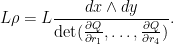
To try to create such a form, we can start with the standard -form

on , and “divide” by the one-forms to create a -form on by requiring that

for , , and , where

Away from the singularities of , the determinant form is non-degenerate (after quotienting out the by the tangent plane , on which this form clearly vanishes). As such, is well-defined as a form on the smooth points of . It also obeys the vanishing condition (7) when one of the is parallel to . However, it doesn’t necessarily obey the scaling relationship (8); instead, one has

for any , where is the quantity

Repeating the heuristic analysis in the introduction, we expect the number of integer points in of height to be , so should morally correspond to “general type” in some sense. This is reflected here by the ability, when , to multiply by an arbitrary homogeneous polynomial of degree , leading to a form which does obey both (7) and (8), and thus descends to an -form defined on the smooth points of . This already shows that for smooth complete intersections , one has general type whenever (because one can use of the form , for a fixed homogeneous polynomial of degree and being the basis functions, to create a portion of the canonical map that is basically the tautological embedding of to ). (Indeed, this argument shows in this case that the canonical bundle on is isomorphic to the pullback of to .)

If has singularities, then the situation is a bit more complicated; we have to pass to the blowup of , and the form may develop some singularities as one approaches the blown up fibres. For the specific blowup considered in Theorem 4, though, it turns out that these singularities are removable, if we make vanish at the exceptional singular points (5); as there are only two such singular points, this will still give enough freedom in to make the canonical map have full dimension in the image.

We turn to the details. Starting with the complete intersection given by (1), we let be the -form on the smooth portion of the deprojectivised variety

defined by the above construction, thus

for a smooth point of , , and . In this case, , , and , so , and so for any linear function , the form descends to a -form on the smooth portion of , which then lifts to a -form on the blown up variety except possibly at the exceptional fibres above each of the singular points of .

We now claim that this -form on can be smoothly continued to each of the fibres if the linear function vanishes at the two exceptional points (5), or equivalently that is a linear combination of the coefficients . Let us first verify this for an obvious singular point. As before, we normalise and , and take the affine chart , then is locally described by the affine variety

where as usual we identify with , and the form restricted to this affine variety takes the form

 

for , , and . In particular, taking for , where is the standard basis, we have

whenever the denominator is non-zero, where is the one-form on that sends a tangent vector to its component , and similarly for , , etc. Using the notation of wedge product , we can write this as

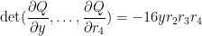
Using (2), we compute that

The quantities are bounded away from zero near the singularity, and is also bounded. Thus we have

 

near the singularity, where we write for -forms to denote the assertion that for some scalar function that is bounded near the singularity.

At first glance, it looks like this form could blow up whenever vanishes, but this does not actually happen as the numerator will also vanish in that case. One can see this by using a different choice of for in (9). For instance, if one takes to be rather than , then we get

and now

so we obtain an alternate form

 

for ; similarly

 

One can also see the equivalence of (10), (11), (12) by noting that 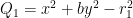vanishes on , which on differentiating yields the linear dependence

between the -forms , which can then easily be used to relate (10), (11), (12) to each other.

Thus the only actual singularity that could occur here is when all vanish. However, it turns out that even here the singularity is removable after blowing up the surface. Recall that the blowup surface takes the form

We pick an affine chart of this surface; for sake of argument we take the chart, as the other charts are treated similarly. Then the surface can be expressed as

with 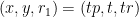. In particular,

and thus

The key point is that there is a common factor of here. Using (11), we thus have

and so does not blow up in the coordinates of as approaches . By Riemann’s theorem, (the pullback of) can thus be extended holomorphically to the exceptional fibre .

Now we look at the behaviour near a non-obvious singularity; for sake of argument we look at the neighbourhood of

As before, we use the affine chart and write , then we are looking at the affine variety

near , where is the system of quadratic polynomials

Applying a change of variables, we have

 

for , , and , and some harmless constant (depending on ). As before, if we set for , we arrive at

 

when the denominator is non-zero. Similarly

 

and

when the denominators are non-zero. Similarly for permutations of the indices.

Now, we lift to the blowup manifold

For sake of discussion we work in the affine chart (say) and write , in which case the manifold becomes

with the convention . To convert back into the original coordinates , we have

and

Thus

and

and thus

Also, . From (14) we can thus cancel all the factors of and conclude that

and so stays bounded up to the exceptional fibre in the blowup coordinates as long as stay bounded away from zero.

It remains to deal with the case when one of the are small. From the form of the curve (6), and the fact that the are in general position, none of the vectors are scalar multiples of each other, which means that only one of the can vanish at a time. Suppose is close to vanishing, so that are comparable to one (the other cases will be similar). In this case, we use (15). As before, and ; also

and so

So once again the factors of cancel, and

and so stays bounded up to the exceptional fibre in this case. Similarly when one of the other are small. Thus stays bounded as one approaches the exceptional fibre in any direction, and so by Riemann’s theorem it can be continued holomorphically to this fibre.

In conclusion, lifts to a smooth -form on the blowup surface . By choosing to be the coordinate functions , we conclude that the image of the canonical map on contains the image of under the (generically defined) projection . But it is easy to see that this map is generically injective on (indeed, one can solve for as rational functions of ), by subtracting the various equations from each other), and so the image has full dimension. This establishes that has general type as required.