This is the third “research” thread of the Polymath15 project to upper bound the de Bruijn-Newman constant  , continuing this previous thread. Discussion of the project of a non-research nature can continue for now in the existing proposal thread. Progress will be summarised at this Polymath wiki page.
We are making progress on the following test problem: can one show that 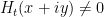 whenever
  ,
,  , and
, and  ? This would imply that

which would be the first quantitative improvement over the de Bruijn bound of  (or the Ki-Kim-Lee refinement of
  ). Of course we can try to lower the two parameters of
  later on in the project, but this seems as good a place to start as any. One could also potentially try to use finer analysis of dynamics of zeroes to improve the bound
  further, but this seems to be a less urgent task.
Probably the hardest case is  , as there is a good chance that one can then recover the
  case by a suitable use of the argument principle. Here we appear to have a workable Riemann-Siegel type formula that gives a tractable approximation for
  . To describe this formula, first note that in the
  case we have
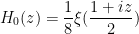
and the Riemann-Siegel formula gives
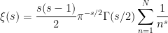

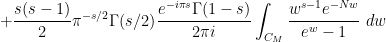
for any natural numbers  , where
  is a contour from
  to that winds once anticlockwise around the zeroes
  of
of  but does not wind around any other zeroes. A good choice of to use here is

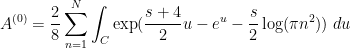
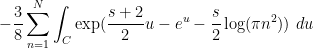
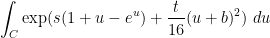
In this case, a classical steepest descent computation (see wiki) yields the approximation

where
Thus we have

where


with  and given by (1).
Heuristically, we have derived (see wiki) the more general approximation

for  (and in particular for
  ), where


In practice it seems that the  term is negligible once the real part
  of
of  is moderately large, so one also has the approximation
For large , and for fixed  , e.g.
  , the sums
  converge fairly quickly (in fact the situation seems to be significantly better here than the much more intensively studied case), and we expect the first term

of the  series to dominate. Indeed, analytically we know that
  (or
(or  ) as
) as  (holding
  fixed), and it should also be provable that
  as well. Numerically with , it seems in fact that
  (or
(or  ) stay within a distance of about
  of
of  once is moderately large (e.g.
  ). This raises the hope that one can solve the toy problem of showing for by numerically controlling
  for small (e.g.
  ), numerically controlling
  and analytically bounding the error
  for medium (e.g.
  ), and analytically bounding both and
  for large (e.g.
  ). (These numbers
  and
and  are arbitrarily chosen here and may end up being optimised to something else as the computations become clearer.)
Thus, we now have four largely independent tasks (for suitable ranges of “small”, “medium”, and “large” ):
- Numerically computing for small (with enough accuracy to verify that there are no zeroes)
- Numerically computing for medium (with enough accuracy to keep it away from zero)
- Analytically bounding for large (with enough accuracy to keep it away from zero); and
- Analytically bounding for medium and large (with a bound that is better than the bound away from zero in the previous two tasks).
Note that tasks 2 and 3 do not directly require any further understanding of the function .
Below we will give a progress report on the numeric and analytic sides of these tasks.
— 1. Numerics report (contributed by Sujit Nair) —
There is some progress on the code side but not at the pace I was hoping. Here are a few things which happened (rather, mistakes which were taken care of).
- We got rid of code which wasn’t being used. For example, @dhjpolymath computed based on an old version but only realized it after the fact.
- We implemented tests to catch human/numerical bugs before a computation starts. Again, we lost some numerical cycles but moving forward these can be avoided.
- David got set up on GitHub and he is able to compare his output (in C) with the Python code. That is helping a lot.
Two areas which were worked on were
- Computing and zeroes for
 around
- Computing quantities like
 , ,
, ,  , etc. with the goal of understanding the zero free regions.
Some observations for , ,  include:
 does seem to avoid the negative real axis
 (based on the oscillations and trends in the plots)
 seems to be settling around
  range.
See the figure below. The top plot is on the complex plane and the bottom plot is the absolute value. The code to play with this is here.

— 2. Analysis report —
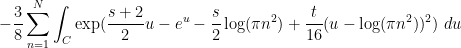
The Riemann-Siegel formula and some manipulations (see wiki) give  , where

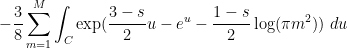

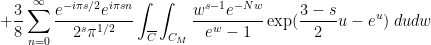
where is a contour that goes from  to staying a bounded distance away from the upper imaginary and right real axes, and
  is the complex conjugate of . (In each of these sums, it is the first term that should dominate, with the second one being about
  as large.) One can then evolve by the heat flow to obtain
  , where


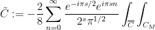


Steepest descent heuristics then predict that  ,
,  , and
, and  . For the purposes of this project, we will need effective error estimates here, with explicit error terms.
A start has been made towards this goal at this wiki page. Firstly there is a “effective Laplace method” lemma that gives effective bounds on integrals of the form  if the real part of
  is either monotone with large derivative, or has a critical point and is decreasing on both sides of that critical point. In principle, all one has to do is manipulate expressions such as
  ,
,  ,
,  by change of variables, contour shifting and integration by parts until it is of the form to which the above lemma can be profitably applied. As one may imagine though the computations are messy, particularly for the
  term. As a warm up, I have begun by trying to estimate integrals of the form
for smallish complex numbers  , as these sorts of integrals appear in the form of
  . As of this time of writing, there are effective bounds for the
  case, and I am currently working on extending them to the
  case, which should give enough control to approximate and
  . The most complicated task will be that of upper bounding , but it also looks eventually doable.


105 comments
Comments feed for this article
12 February, 2018 at 4:48 pm
Terence Tao
In the course of writing down completely effective bounds for oscillatory integrals, I needed a particular effective bound on the Stirling approximation for the Gamma function, namely that
for all in the half-plane
  and some absolute constant
  . From the Stirling series I know that I can asymptotically take
  to be
to be  , but I need a bound which is effective for even relatively small
  (e.g.
(e.g.  ). If anyone knows a reference for effective bounds on Stirling’s theorem that could provide such bounds that would be helpful.
12 February, 2018 at 5:26 pm
Anonymous
Abramowitz & Stegun Handbook gives such bound in 6.1.42
Additional bounds and more recent references can be found in
https://dlmf.nist.gov/5.11
12 February, 2018 at 7:02 pm
David Bernier (@doubledeckerpot)
Section 6.3 of Edwards’ book is entitled: “Evaluation of by Euler-Maclaurin summation, Stirling’s series”. Formula (3) there is Stirling’s series for
  with a remainder term. The remainder term involves the Bernoulli polynomials, defined in Section 6.2 . Edwards writes that the form of the remainder term in formula (3) is attributed to Stieltjes.
12 February, 2018 at 6:22 pm
Sujit Nair
As KM and David pointed out in the earlier thread, computing is expensive at large height.
KM, David, any further thoughts on efficiently computing ?
?
12 February, 2018 at 7:13 pm
KM
Well, right now there are 3 ways to compute H_t. One is the ABC estimate which works well for large scale computations, and the other two are integral approaches (either the original one with cos(zu) in the integrand, or the K_(t,theta) and I(t,theta) derivation). Between the two integral approaches, the latter may do well for larger values of T, but would face the same hurdles after a point, since integrals and such oscillatory functions don’t go well together during computations.
David recently asked in one of the repo threads about a possible Euler Maclaurin approach.
13 February, 2018 at 4:35 am
Anonymous
In the wiki page on asymptotics, in the section “A contour integral”,
  should be
  in the fifth displayed formula and also in the last two lines.
[Corrected, thanks – T.]
13 February, 2018 at 7:09 am
KM
From the perspective of numeric (A+B)/B0 estimates (Task 2) for t=0.4 and y=0.4, they were generated for around a million points x+yi with x between 1 and 1 million, and the behavior at the upper end had turned out to be as expected. Are there any other numerical exercises to be run to complete this task?
13 February, 2018 at 9:08 am
Terence Tao
Two things come to mind. Firstly, for the purposes of bounding the relative error , it appears that it may be slightly more convenient to adjust the definition of
  slightly, first by approximating
  by
by  and then using the Stirling approximation for
  . Thus, the revised definition of
  would be

and similarly
Of course the main term of
of  will similarly adjust to
Presumably the numerical behaviour of should be nearly identical to that of
  once
once  is moderately large, but it is worth checking, as well as testing the accuracy of the
  and
and  approximations to
  at some medium-sized values of
  . It may be that A’ and B’ are in fact a little better to work with numerically in any case, as I would imagine that exponentials and logarithms are slightly faster to compute than Gamma functions. There is an analogous correction to be made to
  , but this term is so small that probably we will be bounding it analytically even for relatively small values of
  so I don’t think it is worth trying to compute it too exactly at this time.
The other thing is not entirely numerical, but we would need to somehow control or
or  between the mesh points as well as on the mesh points. The crudest thing to do is to use some upper bound on the derivative
  or
or  at these points (bearing in mind that the
 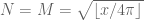 variable has discrete jumps), and hope that the fundamental theorem of calculus bound is enough to keep
  or
or  away from zero outside of the mesh points as well. For instance, we have
and the derivative (bearing in mind that
  , and staying away from the points where
  jumps) contains a term of the form
(plus some terms coming from differentiating the logarithm functions, which I think will be lower order and will thus be ignored for the current discussion) which can be bounded in absolute value using the triangle inequality by
This is just one term in the eventual upper bound for , but it is presumably typical (the other terms are messier though); one could evaluate this at a few values of
  to get some sense of what the derivative might look like, which would indicate what mesh size one would need to keep the function bounded away from zero (basically the mesh size would be the distance from zero at the mesh points divided by the largest value of the derivative).
If it turns out that this simple approach requires a numerically prohibitive mesh size, one could try more advanced things involving control of second or higher derivatives and using a more advanced interpolation formula than the fundamental theorem of calculus (alternatively one could also start computing first or higher derivatives of at mesh points and using some sort of Taylor theorem with remainder).
[Several factors of corrected to
  . -T]
. -T]
13 February, 2018 at 11:14 am
KM
Thanks. I will run the computations along these lines.
14 February, 2018 at 9:48 am
Anonymous
The (truncated) expressions for are “too long” (for one line).
15 February, 2018 at 10:15 am
KM
I think the t in the above formulas should be t/16. Just tested the adjusted formula for some values and the agreement is good (gets much better with higher T)
for eg. for z=1000+0.4j
A+B = -4.794e-168 + 3.127e-167j
A’+B’ = -5.165e-168 + 3.135e-167j
d/dx(B’/B’0) = -0.215 – 0.209j
for eg. for z=100000+0.4j
A+B = -9.32670e-17047 + 4.38004e-17047j
A’+B’ = -9.32705e-17047 + 4.37969e-17047j
d/dx(B’/B’0) = 0.21478 + 0.05395j
15 February, 2018 at 12:44 pm
Terence Tao
Good catch, thanks! (This is one key role that numerics will be playing, by the way – catching sign errors and other typos from the analysis side of things.)
ADDED LATER: By the way, do you have a sense on the relative size of the A and B terms once one is away from the real axis (on the real axis they should of course be complex conjugates of each other). If the A term is much smaller than the B term in practice then we may be able to get away with bounding it by rather crude estimates.
16 February, 2018 at 9:54 am
KM
On evaluating |B/A| in a grid of (x,y,t) where x is powers of 10, we see it increasing at an accelerating pace as x or y or t are increased.
These are some sample values where |B/A| is around 10 for t=0.4
val1=|B/A| for t=0.4
val2=|B’/A’| for t=0.4
val3=|B/A| for t=0.0
z—————val1—-val2—-val3
10^3+1.1i—-11.74—11.74—7.92
10^4+0.8i—-10.55—10.55—5.87
10^5+0.6i—-11.39—11.39—5.05
10^6+0.5i—-11.35—11.35—3.96
10^7+0.4i—-10.75—10.75—3.63
for t=0.4, y=1.3, x=10^5, |B/A| = 132.03
Also, the script evaluating d/dx(B’/B’0) and (A’+B’)/B’0 has been able to run for around 0.7 million points.
Max value of |d/dx(B’/B’0)| seems to be fluctuating but decreasing slowly, while the avg and stdev values decrease more consistently (does not include mesh points which have jumps in N=M)
val=|d/dx(B’/B0′)|
T range——max val—–avg val—–stdev val
———————————————–
upto 1k——1.04——–0.33——–0.19
1k-2k——–1.25——–0.39——–0.24
2k-3k——–1.31——–0.39——–0.25
3k-4k——–1.39——–0.38——–0.27
4k-5k——–1.64——–0.37——–0.26
5k-6k——–1.60——–0.36——–0.27
6k-7k——–1.61——–0.36——–0.26
7k-8k——–1.55——–0.36——–0.27
8k-9k——–1.65——–0.34——–0.26
9k-10k——-1.47——–0.34——–0.26
————————————————–
upto 100k—-1.78——–0.28——–0.23
100k-200k—-1.66——–0.22——–0.18
200k-300k—-1.55——–0.20——–0.17
300k-400k—-1.53——–0.19——–0.16
400k-500k—-1.31——–0.18——–0.15
500k-600k—-1.34——–0.18——–0.14
600k-700k—-1.33——–0.17——–0.14
at z = 28608+0.4i, we get the derivative value (-0.74 + 1.61i) leading to the abs value ~ 1.78 above.
min and max values of the real and imaginary parts of d/dx(B’/B0′) show a similar trend
val = d/dx(B’/B0′)
val1=min(real(val))
val2=max(real(val))
val3=min(imag(val))
val2=max(imag(val))
T range——val1——val2—-val3——val4
——————————————————
upto 100k—-(1.48)—-1.52—-(1.05)—-1.73
100k-200k—-(1.40)—-1.33—-(0.79)—-1.65
200k-300k—-(1.15)—-1.26—-(0.67)—-1.49
300k-400k—-(1.27)—-1.13—-(0.67)—-1.49
400k-500k—-(1.11)—-1.08—-(0.60)—-1.31
500k-600k—-(1.04)—-1.03—-(0.49)—-1.30
600k-700k—-(1.03)—-1.00—-(0.47)—-1.27
Also, for t=0.4, the deviation between (A+B)/B0 and (A’+B’)/B’0 is pretty small after x=1000
val=|(A+B)/B0-(A’+B’)/B’0|/|(A+B)/B0|
T range——max val
————————-
upto 1k——-1.031
1k-2k———-0.009
2k-3k———-0.004
upto 100k—-1.031
100k-200k—-3.548E-05
200k-300k—-1.535E-05
300k-400k—-9.097E-06
400k-500k—-6.636E-06
500k-600k—-4.839E-06
600k-700k—-3.963E-06
In fact the largest value occurs at x=28, and between x=100 to 1000, the average deviation is ~ 1.3%
16 February, 2018 at 8:20 pm
Terence Tao
Thanks for this! Is this the exact derivative of B’/B’_0, or the upper bound for it that I gave previously? I guess it must be the former since the latter wouldn’t oscillate as much as you indicated. In either case it suggests that a unit spacing mesh size will not quite be sufficient to rigorously lower bound (A+B)/B_0 or (A’+B’)/B’_0 in the above ranges, though we “only” have to refine the mesh size by an order of magnitude so we are still within the range of computational feasibility (as long as we don’t have to increase x too much).
It does seem that A is only a smaller than B than one order of magnitude, so we have a little bit of room to estimate A by crude estimates but not too much room. (One could imagine for instance evaluating A on a slightly coarser mesh than B to save on some computing time.)
16 February, 2018 at 10:58 am
KM
Assuming conservatively that |d/dx(B’/B’0)| is around 2, and having observed earlier that |(A+B)/B0| (and hence also it’s adjusted version) starts staying above 0.4 at the integer mesh points consistently beyond x=10^5, can we consider a mesh size of 0.2 between x=10^5 and 10^6 to make the estimates effective for this region?
17 February, 2018 at 10:12 am
KM
Yeah, I had calculated the modulus of the complex valued d/dx(B’/B’_0). On using the triangle inequality estimate for around 0.5 million points, we notice a higher bound (and quite low variance in the bound for a given M).
T range———max of upper bound |d/dx(B’/B’_0)|
upto 30k——–2.320
30k-60k———2.341
60k-90k———2.336
90k-120k——–2.311
————————
upto 100k——-2.341
100k-200k——-2.299
200k-300k——-2.195
300k-400k——-2.109
400k-500k——-2.039
Maximum of 2.341 occurs around x ~ 48000, after which there is a general decline.
With the integer x mesh points, min value of |A’+B’|/|B’_0| is above 0.43 after x ~ 20k (and above 0.39 after x ~ 10k), which suggests a mesh size below 0.15. Having the mesh size as 0.1 would also leave some buffer.
Also, for faster computation of A’ and B’,
using log(z1)^2 – log(z2)^2 = log(z1*z2)log(z1/z2)
and making some manipulations, we can compute B’ as
B’ = B’_0 * sum_(1 to M)_[1/m^(B_exponent – (t/4)logm)]
and correspondingly defining an A’_0 term,
A’ = A’_0 * sum_(1 to N)_[1/n^(A_exponent – (t/4)logn)]
where B_exponent = 1 – s + (t/4)log[(5-s)/(2*PI)]
and A_exponent = s + (t/4)log[(s+4)/(2*PI)]
Since the summation is the bulk operation, and two power operations have been reduced to 1, we expect around a 2x speedup. Running some sample tests, we do observe such a speedup in practice while evaluating H_t as A’+B’.
18 February, 2018 at 3:49 pm
Terence Tao
That’s not as bad as I had feared – it sounds like a mesh size of 0.10 is feasible to work with as long as x doesn’t have to get much larger than , and maybe we can push to
  or
or  with further speedups and maybe some serious computer power. Hopefully the bound on the error estimates begins to become good before this range!
13 February, 2018 at 7:44 am
KM
Also, a separate exercise was run where the normalized stdev of the zero gaps (stdev/avg) was evaluated by estimating a few hundred roots near powers of 10 for multiple t.
normalized stdev for zero gaps (metric)
————-t
T height—-0.50—-0.45—-0.40—-0.35—-0.30—-0.25—-0.20—-0.15—-0.10—-0.05—-0.00
———————————————————————————————-
near 10^3—21.0%—22.2%—23.4%—24.8%—26.3%—27.9%—29.7%—31.7%—33.9%—36.2%—39.2%
near 10^4—13.7%—14.9%—16.7%—18.5%—19.8%—22.0%—24.4%—27.2%—30.6%—34.5%—39.9%
near 10^5—-7.3%—-8.4%—-9.7%—11.2%—13.2%—15.5%—18.3%—21.8%—26.2%—32.0%—40.3%
near 10^6—-4.0%—-4.7%—-5.6%—-6.9%—-8.2%—10.2%—12.9%—16.3%—21.2%—28.1%—40.7%
near 10^7—-2.4%—-2.8%—-3.4%—-4.2%—-5.2%—-6.8%—-8.9%—12.1%—16.3%—23.8%—41.0%
Away from t=0 and as T increases, we get smooth trends in how the metric evolves. This could be used, for example, to predict for a given t at what T height the metric would reach a desired target, say 1%. If there is a rough relation between such T and beyond which the analytically derived zero free region starts, it could also provide a better idea of the expected numerical effort.
Interestingly, for t=0 the behavior of the metric is quite different from that of t>0. It seems to increase as T increases. For t=0, no roots were estimated separately. Instead, 10000 zeta zeroes near each power of 10 were used, as generated by Platt and Odlyzko (which allows us to check the behavior even near 10^22)
normalized stdev for H_0 zero gaps
T height——–metric——-metric using 25th to 75th %tile gaps
near 10^3——39.23%
near 10^4——39.90%
near 10^5——40.30%—–15.75%
near 10^6——40.73%—–16.08%
near 10^7——41.05%—–16.12%
near 10^8——41.48%—–16.44%
near 10^9——41.62%—–16.85%
near 10^10—–41.92%—–16.79%
near 2*10^12–42.03%—–16.75%
near 2*10^21–42.37%—–17.13%
near 2*10^22–41.93%—–16.55%
To counter the GUE distribution effect, and bring it closer to a normal distribution, the same metric was also observed for H_0 gaps lying in the 2th to 75th percentile. While the behavior is weaker, it still seems to be increasing. It may be worth investigating whether such behavior holds for H_0 at even larger values of T.
13 February, 2018 at 7:54 am
KM
Minor correction – that should be the 25th percentile in the last paragraph. Also, the upper table is wrapping around, so posting some plots instead.
https://imgur.com/a/pO9wW
https://imgur.com/a/u2AiR
13 February, 2018 at 9:44 am
arch1
Does the vertical axis of the bottom-right plot need updating? Currently it shows some |C/B0| values as negative.
13 February, 2018 at 10:30 am
arch1
In the expression for , should
  instead be
  ?
?
[Corrected, thanks – in fact there was also factor of 2 in the denominator that was missing also. -T]
14 February, 2018 at 9:52 am
Terence Tao
I think I may have a better way of analytically estimating the various components of than is in the wiki that seems to involve a little less computation. It follows a suggestion made some time back to exploit the fundamental solution to the backwards heat equation
 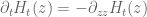 of
of  . It is convenient to work in the
  coordinates, thus
  where
where  solves the forward heat equation
  with initial data
  the Riemann xi function. The fundamental solution then gives
So one is interested in computing expressions of the form
for various meromorphic functions , in particular the terms that arise in the Riemann-Siegel formula such as
  . One can of course use the triangle inequality to bound this by
but this is only a good estimate when does not oscillate too much near
  . It seems that for the error term
  , there is in fact not much oscillation in the total expression (there is a lot of oscillation in individual factors, but it turns out that they largely cancel out in the product) and this could actually be a rather good way of controlling the heat flow for this term. For other terms such as
  , there is a fair bit of oscillation and exponential growth, but one can deal with this by a change of variables. Indeed for each of the terms
  that show up, and at each point
  of interest, there is a complex number
  for which
  behaves like
  in the sense that
for near
near  and some meromorphic function
  that doesn’t oscillate or grow too much near
  . For instance if
  is
is  then
then  can be taken to be
  , basically thanks to Stirling’s formula. After contour shifting
  by
by  (assuming that we don’t run into any poles, but I think this will not be an issue as
  will be relatively small compared to the imaginary part of
  in our application), one can check that the heat evolution
can be rewritten as
(this is related by the way to the Galilean symmetry of the Schrodinger equation). In particular if is so slowly varying that one can approximate
  to high accuracy by
  , then we have
which is basically where the approximation to
  is coming from.
I am cautiously optimistic that all this can be made explicitly effective with reasonable constants, particularly because we can use effective Stirling formula asymptotics which have already been worked out in the literature to deal with all the Gamma function factors. Will work on this.
15 February, 2018 at 8:47 am
Terence Tao
By using some Gamma function estimates of Boyd, I have been able to implement the above strategy to get effective asymptotics (with explicit error terms) for the first two terms of the decomposition
  in the blog post, see this wiki page. This is a work in progress and so one should not take the bounds too seriously yet, but the error term of each summand in
  is about
  of the corresponding term in
  which is a good sign (however, there seems to be significant cancellation in the
  summation and one cannot necessarily assume that there is analogous cancellation for the error terms in the worst-case analysis, so the final relative error may not be as good as this). Similarly for the
  terms. One thing that emerged from the computations is that the approximant to
  that emerges from the heat flow analysis differs very slightly from the original approximation
  and also from the revised version
  above, however I think these differences are inessential (the difference between the various approximations is of order comparable to the error of any of these to the true sum
  ). It seems possible to push the asymptotic computations further and obtain a more complicated approximation with an error that is only
  as large, but this is probably overkill for our application.
To upper bound the final term of the decomposition one will need explicit bounds for the error term in the Riemann-Siegel formula. There is extensive literature on this as long as one stays on the critical line (the main reference seems to be this thesis of Gabke), but we will definitely need estimates away from the critical line and so far I have not been able to locate existing references that do this effectively. However the estimation of this error term is a quite classical steepest descent problem (it’s done in Section 4.14 of Titchmarsh for instance, but not with explicit constants) and it should just be a matter of performing the calculation (though it is slightly annoying because the deformed contour is a weird shape, one needs something that looks a bit like a half-infinite rectangle with a corner cut off, leading to three or four separate integrals to estimate; but all but one of them should be exponentially small).
15 February, 2018 at 9:44 am
Anonymous
In the wiki page on effective bounds on (second approach), it seems that in the definition of
  a second integral symbol is missing, and in the second and third upper bounds on
  , the integrals should be (as already stated there) over the positive axis. Perhaps the resulting bound should be corrected accordingly.
15 February, 2018 at 12:49 pm
Terence Tao
Thanks for the correction! Actually I intended to estimate the gaussian integral on the positive real axis by the integral on the entire line because I have an explicit formula for the latter and not the former. One could be slightly more precise by using the error function erf instead but this leads to an even more complicated bound and I think the gain is rather tiny in practice. (There is definitely a tradeoff in the precision of the error estimate, and how simple the estimate looks. I think it is safe to be somewhat wasteful with lower order errors, such as those of size or
or  times the main term, if it helps in cleaning up the form of the estimate; it is only the main components of the error, comparable to
  times the main term, that are worth being particularly frugal with.)
15 February, 2018 at 12:52 pm
Anonymous
It seems that the paper of Arias de Reyna contains some effective estimation of Riemann-Siegel type formula away from the critical line, see https://pdfs.semanticscholar.org/7964/fbdc0caeec0a41304deb8d2d8b2e2be639ee.pdf .
15 February, 2018 at 7:48 pm
Terence Tao
This looks very useful, thanks! I’ll see what they produce.
16 February, 2018 at 8:37 pm
Terence Tao
I’ve now reworked the computations at http://michaelnielsen.org/polymath1/index.php?title=Effective_bounds_on_H_t_-_second_approach using the Arias de Reyna effective Riemann-Siegel formula to give a completely effective approximation to . It was convenient to change coordinates and write
where with
with  and
and  . The explicit formula for
  is given in the final section of the above wiki. The formula is messy, but the main terms (analogous to the A+B approximation to
  ) are
) are
where
This is a slight variant of the A’+B’ type approximation used previously (which replaced by the slightly different quantity
  , and also took
  to equal
  rather than
  ). It should ultimately lead to almost the same approximation (in much the same way that A+B is close to A’+B’ in practice). The dominant term (analogous to B_0) should be the first term
  in the second sum.
There are three terms in the error estimate. The final term is an integral which should be numerically computable (it depends on a prescribed lower bound for
for  ) and should be quite small (it is analogous to the “C” term). Then there are two other errors called
  which I believe are even smaller expressions. They are given as sums of size N so their computation is about as difficult as computation of the A,B terms, but there is a crude upper bound for these terms in (3.8) of the wiki page which is quicker to compute and possibly might be enough for applications.
This should give a rigorous bound of the form for some variants
  of
of  and some computable
  . If we can get this error
  down to below about 0.4 as soon as
  exceeds say
  then we will be well on track to rigorously keeping
  away from zero for
  .
.
16 February, 2018 at 8:46 pm
Anonymous
Dear Prof. Tao, I am not sure whether there is a sign error in the final bound for H_t in the wiki. The factor e^{\pi T/4} in the last term of (5.1) grows exponentially as T tends to infinity,while H_0 decays exponentially to zero.
[This was indeed a typo – now corrected, I think. Thanks – T.]
17 February, 2018 at 2:52 am
Anonymous
Since for large the integral in the final bound should be (as stated) close to
  , it seems simpler for sufficiently large
  to replace it by a suitable upper bound close to
  (e.g. in
 ![[1.1, 2]](https://s0.wp.com/latex.php?latex=%5B1.1%2C+2%5D&bg=ffffff&fg=545454&s=0&c=20201002) )
)
17 February, 2018 at 5:19 am
Anonymous
for , is this effective approximation to
  sufficiently strong to imply an effective upper bound (as explicit function of
  ) for the real part of any (hypothetical) nonreal zero of
  ?
?
18 February, 2018 at 3:47 pm
Terence Tao
Yes, I believe this should be the case; my preliminary expectation would be that the upper bound to be roughly of the form . It is worth working this out properly at some point, though it probably won’t be directly necessary for the project.
18 February, 2018 at 10:17 am
KM
I have tested the H_t effective approx formula and compared it with the ABC estimate for some values. At large T, the agreement seems good, but some more testing is left. Also, some work is left (the vwf integral) on the error estimation part.
Some minor corrections in the formulas in the comment (they are correct in the wiki):
-> (t/4)*alpha should be (t/4)*alpha^2 (similarly for the conjugate one)
-> alpha_1 won’t have the n^2 factor
-> In the second summation, the exponent should start as 1- sigma – iT instead of 1-sigma+iT (unlike everywhere else in the formula).
18 February, 2018 at 3:52 pm
Terence Tao
Many thanks for the corrections! It’s good that people aren’t just plugging in these formulae blindly, they should definitely be tested numerically and not just taken on faith.
19 February, 2018 at 3:17 am
Anonymous
It is not clear (from its definition) how the new – based approximation gives (approximately) the (previous approximation) main terms of
  (with its exponential decay in
  )
)
19 February, 2018 at 3:25 pm
Terence Tao
It comes from the imaginary part of the logarithm. If with
with  large, then
  has imaginary part close to
  , which gives a contribution of about
  to the real part of
  , which gives a factor of
  in
in  . (See also the Gamma function approximation in equation (1.7) of http://michaelnielsen.org/polymath1/index.php?title=Asymptotics_of_H_t which came from working out the Stirling approximation.)
21 February, 2018 at 1:01 am
anonymous
Do we know how much spare room there is in getting good bounds for ? There are lots of ways to break up for instance the integral of
  , some of them lose quite a bit though. Numerically does this quantity seem to be close to .4 for
  around 10^4, or is it in reality much smaller?
21 February, 2018 at 8:20 am
Terence Tao
Asymptotically this error should be something like I think; numerically I don’t think we have actual data yet, but I am hoping that it is not much larger than
  which was pretty small in practice (ranging between 0.01 and 0.05 in https://terrytao.wordpress.com/2018/02/02/polymath15-second-thread-generalising-the-riemann-siegel-approximate-functional-equation/#comment-492445 ). So we may have about an order of magnitude of spare room.
21 February, 2018 at 2:01 pm
KM
I was facing some problems integrating vwf directly using the inbuilt procedures, so decided to use the Euler Maclaurin approach without derivatives, limits -10 to 10 and h=0.01 (although a smaller limit and larger h also seem to be fine). Since f in vwf rapidly decays on either like a steep bell curve, a low lower and upper limit doesn’t seem to hurt.
Evaluating (|Heff-A’-B’| + |Heff_error|)/|B’0| as a conservative proxy for |H_t – A’ – B’|/|B’0| on some sample values we observe it to be much lower than 0.4 (last column)
(Heff is taken as the sum of the first two terms in the effective approximation, and Heff error as |err1|+|err2|+|err3| of the three error terms)
val1 = |Heff|/|B’0|
val2 = |A’+B’|/|B’0|
val3 = |Heff-A’-B’|/|B’0|
val4 = (|Heff-A’-B’| + |Heff_error|)/|B’0|
t——x——–y——val1–val2–val3——val4
0.4–10000–0.4—0.52–0.52–0.0006–0.039
0.4–12131–0.4—1.28–1.28–0.0004–0.033
0.4–15256–0.4—0.97–0.97–0.0003–0.027
0.4–18432–0.4—0.68–0.68–0.0003–0.023
0.4–20567–0.4—0.98–0.98–0.0004–0.022
0.4–30654–0.4—1.93–1.93–0.0004–0.016
I am now planning to run this with x mesh size of 0.1 for x beyond 10k, and calculate the upper bound d/dx |B’/B’0| at each point as well.
Also, Heff, A’+B’ and A+B-C more or less match even at smallish values of x, but the error estimate in Ht_effective is conservative and increases a lot with decreasing x (last column)
(estimates shown without main exponent term)
t—-x—–y—-ABC—————-A’+B’—————H_eff————%Hf_err
0.4–1k–0.4–(-0.479+3.127i)—(-0.516+3.135i)–(-0.474+3.125i)–27.4%
0.4–5k–0.4–(-1.102+0.141i)—(-1.102+0.140i)–(-1.102+0.141i)—9.5%
0.4–10k—0.4–(-0.692-4.067i)—(-0.687-4.067i)–(-0.692-4.066i)—7.3%
0.4–50k—0.4–(5.443-2.695i)—-(5.443-2.694i)—(5.442-2.695i)—-0.6%
0.4–100k–0.4–(-9.327+4.380i)—(-9.327+4.380i)–(-9.327+4.380i)—0.5%
0.4–150k–0.4–(1.124-0.354i)—-(1.124-0.354i)—(1.124-0.354i)—-0.3%
0.4–200k–0.4–(-1.342-0.098i)—(-1.342-0.098i)–(-1.342-0.098i)—0.2%
Given the three estimates are close to each other, one can be quite confident the repo scripts are correct for Ht_Effective, but having no independent benchmark for the error estimate and the error formulas being complicated, it would be good if others can verify the scripts are computing those correctly (mputility.py in the adjusted_AB_estimates branch).
21 February, 2018 at 3:33 pm
Terence Tao
This is very promising! It seems to indicate that there is indeed a fair amount of room in the error estimates, to the point where we can afford to lose up to an order of magnitude in them and still have a chance of closing the argument (at at least – presumably if we push lower then there will be less room to spare). Do you have a sense of the relative size of the three components of the error? I think err3 should be the largest (and it should be broadly comparable to |C|/|B_0| in magnitude).
For err1 and err2 there is a cruder but simpler bound available (for x large enough) in equation (3.8) of the wiki, it may be that it will suffice for our purposes. As pointed out in a different comment, it would be good to have a cleaner bound for err3; now that I know that we have some room to lose something here it should be possible to do something.
Looking at what we have, it seems the main place where we are still missing something is in Step 3 of the blog post, that is to say bounding (or something analogous like
  ) for large
  , say
, say  . Numerically we have that this expression seems to be staying away from 0, but this could be due to cancellation in the sum. There is a worst-case bound of
  coming from the triangle inequality, which is (if I have computed it correctly)
and if we can get this expression below say 0.9 for say then this may be enough to analytically guarantee no zeroes for
  in this range.
22 February, 2018 at 11:15 am
KM
|err3| is approx an order of magnitude higher than the other two errors in H_t effective, and the ratio keeps increasing as expected.
t=0.4,y=0.4
x———-|err3|/(|err1|+|err2|)
10000—9.11
15000—14.97
20000—19.26
50000—32.39
100000–42.99
10mil—–87.23
The zeta approximation for epsilon errors becomes effective only at larger heights
val = sigma + (t/2)*Re(alpha1(s)) – (t/4)*log(N)
t=0.4
z————val
(10^5+0.4j)–0.7493
(10^6+0.4j)–0.8643
(10^7+0.4j)–0.9794
(10^8+0.4j)–1.0945
The upper bound for |A’+B’-B’0|/|B’0| goes below 0.9 only near x=4*10^7
t=0.4
z—————upper bound |A’+B’-B’0|/|B’0|
(10^6+0.4j)——-2.0498
(10^6+5k+0.4j)—2.0465
(10^6+10k+0.4j)–2.0449
(10^7+0.4j)——–1.2250
(4*10^7+0.4j)——0.8947
(5*10^7+0.4j)——0.8519
(10*10^7+0.4j)—–0.7348
Also, if we check actual values of |A’+B’-B’0|/|B’0| near 10^6 we see it is below 0.9 most of the time, but keeps going over it now and then.
t=0.4
z—————|A’+B’-B’0|/|B’0|
(1026000+0.4j)–1.110910
(1038000+0.4j)–0.948970
(1057000+0.4j)–0.900985
22 February, 2018 at 2:00 pm
Terence Tao
Thanks for this! Hmm, the fact that we only get good analytic bounds beyond is slightly worrying – combined with a mesh size of 0.1 this would mean a fairly intensive numerical computation to control
  up to this scale, unless some speedups are found. (There is an alternative route though, as mentioned in some previous posts, in which we only exclude zeroes
  in a narrow range of
  , e.g.
  , but the price one pays for this is that we need to check all values of
  between
  and
and  , not just
  . But perhaps the effective approximations we have now are usable in these ranges also…
22 February, 2018 at 6:30 pm
Terence Tao
When , one can use approximations such as Stirling’s approximation to find that the expression
  is roughly of the form
where (note: the phase
  has now been corrected)). A model problem is then to find a threshold
  such that one can analytically guarantee the non-vanishing of the above expression (1) for
  (or equivalently
  , where
  ). The triangle inequality bound shows that this occurs as soon as
and this can be verified to be true for larger than
  (with a little bit of room to spare) as in KM's calculations. The question is whether one can do better than this by somehow exploiting cancellation in the phases. It seems that the bulk of the LHS in (1) is dominated by the first few terms of the first sum, which suggests a couple of potential strategies:
1. Numerically compute just the first few terms of (1) (which should be a lot faster than computing the whole thing) and use the triangle inequality for the rest. to get some lower bounds on the real part of (1) that improve upon the triangle inequality, for instance by lower bounding the net contribution of the n=1, n=2, and n=4 terms in the first sum of (1).
 to try to partially cancel off some terms.
2. Try to use trig identities such as
3. Multiply the LHS of (1) by some factor such as
22 February, 2018 at 10:54 pm
Terence Tao
Looks like strategy 3 can cut down the threshold for x by about an order of magnitude (i.e. it can handle ). To make (1) non-zero it suffices to show that
Multiply both sums by (the point being that this cancels off a large portion of the contribution of the even
  to the sum). The sum in the LHS becomes
and the sum in the RHS similarly becomes
So by the triangle inequality we now win if
Numerically this seems to occur for close to 500 (so
  close to
  ). I would expect similar results for other versions of the
  expression that we have discussed previously.
In principle one could obtain a further improvement by also multiplying through by , but the calculations get messy and I doubt one would have as dramatic a gain in
  as a consequence. It does show though that the
  do retain some partial vestige of an Euler product, which I did not expect.
23 February, 2018 at 11:10 am
KM
4*10^6 is much more manageable numerically than 4*10^7 :)
At x=pi*10^6, the triangle inequality bound is 0.976, while at 3.5*10^6, it goes below 0.95. Stopping numerically here would cut down the computation time further by about 10-20%
I also checked for z=4*10^7+0.4j, the t value till which H_t effective is useful. The error at t=10^-8 is around 19%, below which the error term increases quickly.
t———-%error in H_t_eff
10^-9—60.9%
10^-8—19.3%
10^-7—-6.1%
0.01——0.2%
0.1——–0.09%
0.4——–0.0016%
24 February, 2018 at 3:46 am
KM
Not completely sure about the derivation below, but if we follow the template and multiply the 1-1/3^() factor, we get triangle inequality eqns like below
where we then have to find the threshold for L + R < 1
Similarly, if we multiply 1-1/5^(), we get 8 conditional factors in both L and R, with the final one in R being
Using this, the eqn with 3 multiplication factors just goes below 1 at x=1 mil.
Also, I noticed that while calculating the inequality, we did not divide back by a factor like
which would again increase the LHS. If we divide back by the factors used, we get these results. The eqn with 3 multiplication factors is around 0.965 for x=5.5 mil.
x———orig—fac2–fac2,3–fac2,3,5
[2.5mil, 1.68, 1.44, 1.33, 1.29]
[3.0mil, 1.61, 1.36, 1.25, 1.21]
[3.5mil, 1.56, 1.30, 1.19, 1.14]
[4.0mil, 1.51, 1.25, 1.13, 1.09]
[5.0mil, 1.44, 1.17, 1.05, 1.00]
[5.5mil, 1.41, 1.14, 1.01, 0.96]
[6.0mil, 1.38, 1.11, 0.98, 0.93]
[6.5mil, 1.35, 1.08, 0.95, 0.91]
[10 mil, 1.23, 0.95, 0.82, 0.77]
[40 mil, 0.89, 0.62, 0.49, 0.45]
24 February, 2018 at 8:07 am
Terence Tao
Thanks for this! I think we don’t need to pay factors like because they appear on both sides of the inequality. So the gain may be slightly more than indicated. Still it seems from your preliminary analysis that the additional savings from adding in the 3 and 5 primes are perhaps worth the increased complexity.
14 February, 2018 at 10:59 am
Vassilis Papanicolaou
(I’ve just posted this comment at Thread 1. I am reposting it here, since it seems that the attention has shifted to Thread 3).
I would like to share few rough ideas regarding the dynamics of the zeros z_j(t) of H_t(z):
It seems clear that H_t(z) is entire in both z and t. Hence the zeros z_j(t) are the branches of a global analytic function, say Z(t), defined on an infinite-sheeted Riemann surface S. The projections of the branch points of S on the complex plane are the values of t for which we will have multiple zeros of H_t(z), and these are countably many points, say t_k, k = 1, 2, … (possibly without accumulation points in the complex plane). Then, by analytic continuation one expects that the equations giving the dynamics of the zeros will continue to hold (in some sense?) for any complex t, except at t = t_k.
14 February, 2018 at 1:53 pm
Anonymous
Any simple zero has a local representation by its (locally convergent) Taylor series, while multiple zeros are locally represented by the locally convergent branches (around each branch point
  ) of their Puiseux series, see
https://en.wikipedia.org/wiki/Puiseux_series
14 February, 2018 at 2:23 pm
Anonymous
The current proof of the ODE Dynamics of zeros depends on the fact that H_t is an even entire function of order less than
  (needed for its simple form of Hadamard factorization) for any real
  . It is not clear if
  has all these properties for some non-real
  .
.
15 February, 2018 at 12:28 am
Vassilis Papanicolaou
Thanks for the comments. I will try to check the order and the evenness of for non-real
  . I suspect that the order is not affected by the imaginary part of
  .
. -order (and type) of
  known for any real
  ?
? -order of
  (possibly 1 of infinite type?). Then, it may be helpful to look at the zeros
  .
.
If I may ask, is the exact
Also, it should not be hard to estimate the
15 February, 2018 at 8:36 am
Terence Tao
On page 2 of the Ki-Kim-Lee paper it is noted that (which is related to
  by the simple transformation
  is of order 1 and maximal type because it is the Fourier transform of an extremely rapidly decaying function (this is an application of the Paley-Wiener theorem). It looks to me like this argument would also apply for complex values of
  .
.
16 February, 2018 at 2:59 am
Vassilis Papanicolaou
Thanks for the reply!
14 February, 2018 at 1:04 pm
David Bernier (@doubledeckerpot)
It seems as though there may already be a Python procedure that can do Gauss-Legendre quadrature, which is the method I use to evaluate by integration.
Reference and link:
https://en.wikipedia.org/wiki/Gaussian_quadrature
and
https://docs.scipy.org/doc/scipy-0.14.0/reference/generated/scipy.integrate.quadrature.html
14 February, 2018 at 3:44 pm
Rudolph
I have played quite a bit with the ABC-approximation formula for and managed to produce some ‘x-ray’-plots (also called ‘implicit plots’) that show all points on an x,y-plane where
  and
and  . The first plot just illustrates how well the approximation formula works for
  around the first Lehmer pair (zeros reside at those points where the red and green lines cross):
https://ibb.co/fe9AGS
The second plot shows the evolution of this Lehmer pair when varies. Note that the Lehmer-phenomenom becomes more or less invisible when
  . I fully realise the focus is on the positive domain
  , however the approximation formula appears to continue to work pretty well for negative t.
The bottom row of the plot shows the 'birth' of a pair of zeros off the critical line (and it happens indeed 'barely' below ).
).
https://ibb.co/eNQT37
Note that the imaginary lines (red) are much better behaved (and spaced) than the real ones (green). Two subsequent red lines seem to constrain the 'wiggle room' for the green lines to stay on the critical line. Based on this observation, I wrote a root finding program that first establishes two subsequent red points on a line just above the x-axis at and then uses these as the precise interval for the pari/gp solver to establish where a real (green) line crosses the x-axis at
  . This method automatically revealed the zero pair: 2*5229.198 and 2*5229.242 (also found by David and KM) that lies just above the x-axis (note this is clearly an approximation error, not a zero lying off the line :-) ). In these cases, the algorithm just spots two subsequent empty 'bins', so there is no need to check back against the known non-trivial Riemann zeros to spot a missing pair (which can't be done for t larger than 0 anyway). This method is of course slower (since it requires two solving steps) than the root finders proposed earlier, however it is less sensitive for accidentally "jumping over" e.g. a Lehmer pair when the step size for finding the next sign change is set too large.
14 February, 2018 at 9:15 pm
Anonymous
Very interesting graphs. I remember Csordas et al. used an extreme Lehmer pair near Im z=388858886.00228512… and Im z=388858886.00239368… to produce a lower bound of de Bruijn-Newman constant. Is it possible to produce similar “X-ray” graphs near these two zeros?
15 February, 2018 at 8:06 am
Rudolph
Sure, will try to run the plots (note that at these heights of x the processing is time required is considerable, I expect to have to scale down the plotting resolution a bit).
Thanks for this extreme Lehmer pair, since it provides a great opportunity to test my root finding algorithm. Searching for zeros from 388858885 to 388858887, using a step size of 0.1 and the line 2*(x+0.01y) to establish the search intervals, I found for t=0 and the full ABC-approximation (numbers truncated at 6 decimals):
388858885.231056
388858885.384337
388858886.002152
388858886.002526
388858886.690744
388858886.891322
388858887.016571
However, without the C-factor, this Lehmer pair lies just above the x-axis, but its absence is automatically spotted:
388858885.232052
388858885.383403
no zero between: 388858885.648782 388858886.002360
no zero between: 388858886.002360 388858886.346191
388858886.691773
388858886.888967
388858887.018302
It seems that for root finding purposes the C-factor remains important even at higher values of x.
15 February, 2018 at 10:58 am
KM
I think at large heights, the C factor would be important for t=0 where Lehmer pairs exist, but would probably not be critical away from t=0 where the gaps get more regular. Corresponding zeroes for this zero pair may be worth checking for t small, say 0.05 or 0.1 and t large, closer to 0.5, with and without using C.
16 February, 2018 at 2:57 pm
Rudolph
Here are the ‘x-ray’ plots that show the evolution of the Lehmer pair 388858886.00228512, 388858886.00239368. For the graphs I have used the Sagemath (implicit) plotting capability and for the computations Pari/GP. Each graph took roughly 6 hours to complete on my 2013 iMac (i5 CPU). No doubt this can be sped up with better hardware. The last three plots have been processed in parallel in the Cocalc cloud (they have a slightly different color), however they still took about the same time to generate. Compared to the previous plot, I reduced the plot-point density from 150 to 60 to keep computing time in a ‘decent’ range.
https://ibb.co/doqBAn
Few observations: approximation formula remains valid, however this needs to be confirmed.
 -threshold after which the Lehmer pair is no longer found). This is already significantly lower than t=-0.000825 where about the first Lehmer pair collision occurs (see these graphs for a zoomed-in view of that actual collision: https://ibb.co/g9OxgS ).
 graph now also shows that the imaginary (red) lines could bend ‘to the left’ (like the real lines already did for the upper member of a Lehmer pair).
 , the ‘wrinkles’ in the lines induced by a Lehmer pair, seem to get ‘ironed out’ much faster when
  moves up from
  , compared to Lehmer pairs at lower heights of
  . If this is true, then this indeed could be another indication that a mix of computation up to a certain height and an analytical solution above that, is a promising approach to reduce the upper bound of
  . I’ll try to produce a (low resolution) plot for a Lehmer pair in the
  domain to see if this effect remains.
1) For negative t, I assumed the
2) Assuming 1), the collision of the Lehmer pair occurs somewhere between t=-0.0000000688 and t=-0.0000000689 (I used the root finder to establish the
3) The
4) Apparently for increasing heights of
16 February, 2018 at 3:09 am
Anonymous
In the wiki page “effective bounds on “, what is the precise meaning of
  ?
?
[This is now explained in a rewritten version of the page – T.]
16 February, 2018 at 9:37 pm
David Bernier (@doubledeckerpot)
I did some computations of for
for  from 160 to 3200, by increments of 160. This took 4 hours for 20 points.
The command to PARI/gp was:
for(K=1, 20, x50= K*160 ;
s=0.0;
for(J=0,30,
s=s+intnumgauss(X=J/13,(J+1)/13, exp(t*X*X)*Phi(X)*cos((x50)*X),));
s2=H(x50);
b0=HM(x50);
s4 = abs((s2-s)/b0);
w20[K] = s4;)
Thus, for each point , I did 31 Gauss-Legendre quadratures, each over an interval of length 1/13, and summed the 31 values.
 real with z>100, the time to compute
  by the integral method increases roughly like
  .
.
Also, for
The output is copied below:
? for(K=1,20, print(K*160,” “, w20[K]))
160 0.06993270565802375041
320 0.006716674125965016299
480 0.005332893070605698501
640 0.003363431256036816251
800 0.1548144749150572349
960 0.03009229958121352990
1120 0.004507664238680722472
1280 0.002283591962997851167
1440 0.01553727684468691873
1600 0.001778051951547709718
1760 0.02763769444052338578
1920 0.002108779890256530964
2080 0.02746770886040058927
2240 0.001567020041379128455
2400 0.01801417530687959747
2560 0.001359561117436848149
2720 0.008503327577240081269
2880 0.001089253262122934826
3040 0.003004181560093288747
3200 0.02931455383125538672
17 February, 2018 at 8:08 am
David Bernier (@doubledeckerpot)
I see that in mpmath, there is a way to divide up the interval of integration into sub-intervals;
copied from:
http://mpmath.org/doc/current/calculus/integration.html :
“One solution is to break the integration into 10 intervals of length 100:
>>> quad(sin, linspace(0, 1000, 10)) # Good
0.437620923709297 ”
The answer is 1-cos(1000) ~= 0.437620923709297.
I might try in Python interactively.
18 February, 2018 at 3:44 pm
Terence Tao
Looks reassuringly small, though the spike at x=800 is weird and I don’t have any plausible explanation for it.
19 February, 2018 at 5:08 am
David Bernier (@doubledeckerpot)
My preliminary analysis is that the quotient has jump discontinuities for values of of the form
  for positive integers n, including at
  and
and  , which is about 804.247. The error goes from moderate to small across the discontinuity:
 .
.
x50=256*Pi-0.0001;
s=0.0;for(J=0, 50, s=s+intnumgauss(X=J/15, (J+1)/15, exp(t*X*X)*Phi(X)*cos((x50)*X),));s2=H(x50); b0=HM(x50); s4 = abs((s2-s)/b0);s4
= 0.17313
and:
x50=256*Pi+0.0001;
s=0.0;for(J=0, 50, s=s+intnumgauss(X=J/15, (J+1)/15, exp(t*X*X)*Phi(X)*cos((x50)*X),));s2=H(x50); b0=HM(x50); s4 = abs((s2-s)/b0);s4
= 0.00305 .
For the choices I make in the Riemann-Siegel formula, both M and N have discontinuous jumps for
19 February, 2018 at 12:27 pm
David Bernier (@doubledeckerpot)
It might be worth studying numerically the size of the discontinuities in , where
  have jumps. I find semi-empirically that the Riemann-Siegel approximation to
  has discontinuities for
  . The reason to look at the size of discontinuous jumps in
  is that Terry’s Riemann-Siegel formula is much faster to compute than the integral that defines
  . The idea being that hopefully the discontinuities could be useful proxies for the error in the
  formula with respect to the integral defining
  .
.
19 February, 2018 at 12:50 pm
Anonymous
If the sizes of the discontinuities can’t be explained by the (effective) upper bound on the remainder term, this would indicate that there is an error in the formula.
19 February, 2018 at 1:51 pm
David Bernier (@doubledeckerpot)
Here is what I got for the absolute values of the discontinuous jumps in , relative to the continuous
  :
:
for(JJ=3, 8,K=2^JJ;
x50= 4*Pi*(K^2) ;
s2=H(x50-epsilon);
s3= H(x50+epsilon);
b0=HM(x50);
s4 = abs((s2-s3)/b0); // s4 is abs. rel. jump
print(x50,” “,s4))
x50: s4:
———————-
804.247 0.176
3216.990 0.0375
12867.963 0.00794
51471.854 0.00159
205887.416 0.000295
823549.664 5.028 E-5
epsilon
1.000 E-20
Note: No use is made of the integral formula for above.
19 February, 2018 at 3:37 pm
Terence Tao
Interesting! The “C” term has the property that it also has discontinuities at these places, but the jumps in the “C” term are supposed to largely (but not completely) cancel the jumps in the “A” and “B” terms. So presumably things would be much worse near these discontinuities if we only had the A+B term. I do indeed agree that it is worth studying the numerical behavior of in the vicinity (and in particular on both sides) of say
  , as this looks like it will give the worst-case behaviour with regards to accuracy of approximation. (Certainly this is where the
  term should be largest in magnitude; it should roughly be the size of the final summand in the A or B terms.)
EDIT: it seems from your more recent data that the size of the jump in A+B-C decays rather rapidly as x increases, so it seems the cancelling effect alluded to above is kicking in but only for largish x.
19 February, 2018 at 5:10 pm
David Bernier (@doubledeckerpot)
Some more data of the form log( | jump/B_0 |)/log(x), for x from to
to  ; it shows a steady decrease from -0.259 to -0.836:
for(JJ=3, 10,K=2^JJ;
x50= 4*Pi*(K^2) ;
s2=H(x50-epsilon);
s3= H(x50+epsilon);
b0=HM(x50);
s4 = abs((s2-s3)/b0);
s5=log(s4)/log(x50);
print(x50,” “, s5))
x: s5:
804.247 -0.259
3216.990 -0.406
12867.963 -0.511
51471.854 -0.593
205887.416 -0.664
823549.664 -0.726
3294198.658 -0.783
13176794.633 -0.836
19 February, 2018 at 7:48 pm
David Bernier (@doubledeckerpot)
I did for what I did previously for
  . What I find numerically is that the jump discontinuities in
  , relative to
  decay faster for
  than for
  … This is for
  to
to 
t=0.0;
for(JJ=3, 10,K=2^JJ;
x50= 4*Pi*(K^2) ;
s2=H(x50-epsilon);
s3= H(x50+epsilon);
b0=HM(x50);
s4 = abs((s2-s3)/b0);
s5=log(s4)/log(x50);
print(x50,” “, s5))
x: s5:
804.24 -0.194
3216.99 -0.311
12867.96 -0.384
51471.85 -0.434
205887.41 -0.471
823549.66 -0.500
3294198.65 -0.524
13176794.63 -0.543
22 February, 2018 at 6:01 pm
David Bernier (@doubledeckerpot)
Here are some results for , in absolute value, for x ranging from
  to
to  , going by increments of
  in x; the largest of these is for
  in the next-to-last row:
622.035345 0.003667321
631.460123 0.004268055
640.884901 0.003284407
650.309679 0.004453589
659.734457 0.003872174
669.159235 0.005048162
678.584013 0.005009254
688.008791 0.007418686
697.433569 0.007464541
706.858347 0.010692337
716.283125 0.012938629
725.707903 0.017830524
735.132681 0.022428596
744.557459 0.030907876
753.982237 0.040060298
763.407015 0.053652069
772.831793 0.071092824
782.256571 0.094081856
791.681349 0.123108726
801.106127 0.159299234
810.530905 0.002870724
16 February, 2018 at 10:19 pm
Vassilis Papanicolaou
The de Bruijn function is entire in
  and it obviously satisfies
  , i.e. it is even in
  .
.
Furthermore, as a function of ,
,  is of order
  (and of maximal type) for any complex
  .
.
(It seems, too, that as a function of ,
,  is of order
  (and of maximal type) for any complex
  ).
).
The zeros are analytic in
  except at certain (branch) points
  ,
,  , where two zeros cross.
In the G. Csordas, W. Smith, and R.S. Varga (1994) paper it has been shown that if is real and
  , then the zeros are (real and)
simple and satisfy the dynamics
Since , is even in
  , we have that
  is a zero of
  if and only if
  is a zero (counting multiplicities, of course).
Hence, the above dynamics can be written as
(we can also multiply by and get the dynamics of
  ). Since
  is of order
  , the last sum above converges absolutely. Therefore, by analytic continuation, the above dynamics should continue to hold for any complex
  .
.
18 February, 2018 at 7:56 am
K
Dear Vassilis, you can use inbuilt latex with DOLLARlatex … DOLLAR, for example when you write DOLLAR latex \frac{x}{y}DOLLAR, it compiles to
20 February, 2018 at 1:10 am
Vassilis Papanicolaou
Thanks! Does the same work for displayed formulas?
[The latex parser here does not recognise environments such as \begin{equation}…\end{equation}, but it accepts the \displaystyle command at least. -T.]
21 February, 2018 at 12:40 am
Vassilis Papanicolaou
Thanks!
17 February, 2018 at 3:56 pm
Rudolph
@Vassilis,
I had already wondered about what would happen when we make and hadn’t appreciated that analytic continuation works for all
  .
.
Therefore made some X-ray plots to visualise how a Lehmer pair would respond to changes in . Below are the ‘collision’ plots for respectively
  and
and  when
when  varies:
https://ibb.co/fAL3rS
https://ibb.co/mNnYrS
Note: the plots for are just versions mirrored over the x-axis.
Also checked at which the collision would happen for the larger Lehmer pair (388858886.00228512, 388858886.00239368) and that is at about
  (compared to
  for the first Lehmer pair).
It seems that zeros already move off the critical line at pretty small and this might be an early indication that defining a complex
  with for instance an associated complex
  doesn’t look to be a very promising route. However, when
  is complex the ‘red lines’ do start to move when
  changes. I found that for any
  , there is a corresponding
  where now the red lines will collide (almost like an ‘echo’ of the Lehmer pair collision on the real line just below it). I produced the attached graph for
  to illustrate this observation:
https://ibb.co/ksw7kn
P.S. for latex to work on this forum, just put dollarlatex in front and a single dollar at the end of your code (substitute the dollar sign where I wrote dollar).
17 February, 2018 at 6:50 pm
Michael Ruxton
0 + ib with b = 0.025 or b = 0.0025 ?
18 February, 2018 at 2:24 am
Rudolph
Good catch. It is 0.025 of course. Corrected graph below.
https://ibb.co/dWbrvn
22 February, 2018 at 12:06 pm
Doug Stoll
You chose a good early example .
Are you also able to examine the pairs starting at:
10854395965.14210 with actual gap to next zero of 0.00002420
1239587702.54745 with actual gap to next zero of 0.00007356 and the numerically challenging one way out at
1034741742903.35376 with actual gap of 0.00001709
Thank you.
18 February, 2018 at 4:06 am
Vassilis Papanicolaou
Dear Rudolph,
Thanks for the reply. One strategy, then, to approach RH maybe the following: The zeros of
of  are the branches of a global analytic function
  defined on an infinite-sheeted Riemann surface
  .
.
If (i) the set of ramified points of is discrete and (ii) the ramification indices of these points are finite, then
  has at most finitely many nonreal zeros.
(I hope I did corrrectly what you indicated to me regarding the latex appearance).
18 February, 2018 at 4:26 am
Vassilis Papanicolaou
Sorry,
instead of “(ii) the ramification indices of these points are finite”
I meant to say that there are only finitely many points on whose projection on the complex plane is
  (at least for each real
  ,
,  .
.
This is somehow in accordance with the Ki-Kim_Lee paper.
18 February, 2018 at 11:07 am
Anonymous
It seems that the extreme difficulty of RH indicates that (probably) (ii) does not hold (but RH is still possible, of course.)
17 February, 2018 at 4:26 pm
Anonymous
Dear Terry,
If this project pulls about 100 mathematicians,the Riemann problem can be solved soon
19 February, 2018 at 6:48 am
Anonymous
In the main wiki page, it seems that should be “non-increasing” (instead of “non-decreasing”).
[Corrected, thanks -T.]
19 February, 2018 at 11:05 am
Anonymous
For (by the KKL paper), any nonreal zero of
  is simple. Is it possible by the new effective approximation to
  to derive an effective positive lower bound (as explicit function of
  ) for the distance of any nonreal zero of
  from the other zeros of
  ?
?
Such a bound should imply (via the zeros ODE dynamics) an effective upper bound on the velocities of the nonreal zeros of – which can be used to establish a zero-free domain of
  from a known zero-free domain of
  .
.
It seems that the current difficulty for establishing such zero-free domain for is the lack of such an effective upper bound on the horizontal velocities of incoming nonreal zeros of
  into a known zero-free domain of
  .
.
19 February, 2018 at 3:31 pm
Terence Tao
Unfortunately Theorem 1.3 of KKL only ensures that all but finitely many zeroes are simple at any given time ; it looks like one could make this more effective now by giving an explicit value
  such that all zeroes of real part greater than
  are both real and simple. However we don’t seem to have any way to prevent a finite number of collisions at medium-sized real parts and non-zero imaginary parts in which the approximations available are not useful. Probabilistic heuristics would suggest that this does not happen (basically because the set of polynomials of a given degree with real coefficients but a repeated complex zero has codimension 2 and the heat flow is a trajectory of dimension 1) but I don’t see a mechanism to rule it out a priori.
20 February, 2018 at 12:00 am
Anonymous
It seems that in the wiki page on effective bounds on (second approach) there are certain errors
1. In the (first) definition of , it seems that
  should be
  (to ensure that
  remains real and non-negative as required by the definition of
  ). [In the discussion here it is assumed that
  is positive (in fact it is at least
  ). -T.]
2. In the definition of , it is complex (which seems incompatible with the bounding of
  which seems to assume
  to be real, and also with the second definition of
  by complex
  ). [The
  was a typo, now corrected – T.]
20 February, 2018 at 12:52 pm
Anonymous
Another typo: in the third integral bound on , it should be
  (instead of
  ).
).
[Corrected, thanks – T.]
20 February, 2018 at 11:49 pm
anonymous
Another small typo, at the end (in section ‘Final bound’): it should read that `f is defined by (4.1)’ rather than (4.8). Also in (4.1) there is an errant ‘du’.
[Corrected, thanks – T.]
20 February, 2018 at 1:07 am
Vassilis Papanicolaou
In my comment regarding the dynamics of the zeros (February 16 2018, 10:19pm) there was an ERROR. Here is the corrected version:
In the G. Csordas, W. Smith, and R.S. Varga (1994) paper it has been shown that if is real and
  , then the zeros are (real and) simple and satisfy the dynamics
Since , is even in
  , we have that
  is a zero of
  if and only if
  is a zero (counting multiplicities, of course). Hence, the above dynamics can be written as
or
We can also multiply by and get the dynamics of
  :
:
Since is of order 1 (and, being even,
  , where
  is entire of order
  ), the last sum above converges absolutely. Therefore, by analytic continuation, one expects that the above dynamics should continue to hold for any complex
  , where
  are the branch points.
21 February, 2018 at 1:05 pm
Anonymous
In the wiki page on effective bounds on (second approach), is there a simple bound (for moderately large
  ) for the integral in the final bound (to simplify its numerical computation)?
21 February, 2018 at 5:07 pm
Anonymous
It is not clear from the final bound, what is the relative magnitude of the integral error term with respect to the main term of (i.e. its asymptotic decay rate for large
  relative to the magnitude of
  ).
).
22 February, 2018 at 1:55 pm
Terence Tao
The expression has size about
  , so the first term (now called
  in the wiki) should have size about
  times the sum
  (which is bounded in practice, but analytically can only be bounded efficiently currently for large
  ). Similarly, the second term (now called
  ) has size about
  times
times  . The main term here (call it
  has magnitude about
  . Of the error terms (now called
  on the wiki), the first term should be about
  in size (so about
  of
of  ), the second term should be about
  in size (so about
  of
of  ), and the third should be about
  in size (so about
  of
of  ). This seems broadly consistent with the numerical data showing that
  is the most significant error.
22 February, 2018 at 1:48 pm
Anonymous
It seems that the jumps near are due to
  in the denominator of the expression for
  which (because of rounding errors) should be computed more accurately near the removable singularities
  (for which both the numerator and denominator nearly vanish – therby loosing many significant digits!)
22 February, 2018 at 2:53 pm
Anonymous
Since is currently considered to be an error term, I think now that most probably, the jumps are due to jumps in the value of
  (i.e. when
  is an integer.
 ) by refining the current estimate to include the detailed influence of
  (i.e. not considering it as a merely “error term” – as done in the current estimate)?
Is it possible to reduce these jumps (and the size of
22 February, 2018 at 5:33 pm
Terence Tao
Yes, this amounts to using an “A+B-C” type approximation to rather than the “A+B” approximations that we are currently discussing. It seems though that the C term is in practice one or two orders of magnitude less than the A and B terms, so this level of precision is probably not necessary for our application (though it would be helpful for looking at dynamics of zeroes, as some other commenters have done).
23 February, 2018 at 3:07 am
Anonymous
I still think that contribute the “main term” to the error term
  . To show that, note that
appearing in the integral representation of can be represented as
where , and
, and
Since
Where the error term is effective, it is clear that
  contribute the main term to the integral representation of
  (with relative error of
  ).
).
Hence, my suggestion is to first extract the contribution of (i.e. the “main term”) to the integral representation of
  , and only then bound the remaining terms (which are
  relative to the already extracted “main term”).
23 February, 2018 at 7:42 am
Terence Tao
I agree that the term will be the dominant contribution to the
  portion of
  , and extracting it amounts more or less to replacing the “A+B” type approximate functional equation currently used with an “A+B-C” refinement. However, relative to
  , it seems numerically that A+B has magnitude at least 0.4 or so, while C has magnitude about 0.01, and the upper bounds for the error including C are only a little larger at 0.02 or 0.03. So at present it seems there is not a pressing need to refine the approximation by extracting the “C” term. However one may well need to do so if one later aims to lower the value of t or y.
23 February, 2018 at 12:51 pm
Anonymous
In the wiki page on effective bounds on (second approach), in the section “Bounding
  “, it seems that the argument
  appearing (5 times in the section) in
  should be
  .
.
[Corrected, thanks – T.]
23 February, 2018 at 10:15 pm
Terence Tao
I will roll over the thread shortly, but just a heads up that I am in the process of writing a new wiki page http://michaelnielsen.org/polymath1/index.php?title=Polymath15_test_problem on the problem of showing that whenever
  . So far I have written the four A+B type approximations we have available (finding some typos in the definition of the “toy” approximation in particular) and computed some numerical values. It looks like all of the approximations are in good agreement. Tomorrow I will try to input some of the other data that other commenters have made on the approximation and then write a fourth thread post for the polymath project.
24 February, 2018 at 1:38 am
Anonymous
It would be interesting to see (for each type of approximation) the explicit functional relationship between and
and  .
.
24 February, 2018 at 8:09 am
Terence Tao
I think in all cases the equation is (or, if one extends
  to the lower half-plane by reflection,
  ).
).
24 February, 2018 at 1:52 am
George Szekers
Dear Terry,
In your page please change /\ < = 0.96 to /\ <= 0.48
(
this is below the definition of the test problem, line 5 in the document
http://michaelnielsen.org/polymath1/index.php?title=Polymath15_test_problem
)
[Corrected, thanks – T.]
24 February, 2018 at 2:20 am
Anonymous
In the wiki page on the test problem, the (expected) new upper bound should be 0.48 (instead of 0.96).
24 February, 2018 at 10:08 am
Polymath15, fourth thread: closing in on the test problem | What's new
[…] thread of the Polymath15 project to upper bound the de Bruijn-Newman constant , continuing https://terrytao.wordpress.com/2018/01/24/polymath-proposal-upper-bounding-the-de-bruijn-newman-cons…. Progress will be summarised at this Polymath wiki […]