
This is the ninth “research” thread of the Polymath15 project to upper bound the de Bruijn-Newman constant 
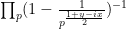
We have now tentatively improved the upper bound of the de Bruijn-Newman constant to 


The main remaining bottleneck is that of computing the Euler mollifier bounds that keep 

Participants are also welcome to add any further summaries of the situation in the comments below.

84 comments
Comments feed for this article
4 May, 2018 at 3:38 pm
Anonymous
Can the more precise approximation be helpful in reducing the computational complexity?
 is much smaller than
  ) that a better strategy is to try reducing
  (e.g. to 0.15) and allow increasing
  (e.g. to 0.3) to keep reasonable computational complexity?
Is it possible (since
5 May, 2018 at 2:26 am
KM
These are some of the ongoing numerics threads:
1) Testing the mollifier approximations at N=69098, y=0.2 t=0.2. The triangle bounds are quite negative, so lemma bounds and its approximations are needed. A prime only mollifier with enough Euler factors (for eg. Euler 41 or Euler 61) seems to come close to the performance of a full mollifier, but due to the larger number of primes needed does not give a speed advantage. The lemma bound is currently being approximated by using the lemma on the first N terms and the triangle bound tail sum for the remaining D*(N-1) terms. This mixed approximation is not as effective as a potential fully lemma based approximation, but the latter doesn’t seem easy to derive. The approximation is almost as fast to compute as a non-mollified bound, but did not turn positive.
Some sample bound estimates (T: Triangle bound, L: Lemma bound):
N=69098,y=0.2,t=0.2
T E5 full_moll : -0.1264
T E5 full_approx : -0.2155 (current approx is minimum here)
T E5 prime_moll : -0.2350
T E5 prime_apprx: -0.2509
T E13 prime_moll: -0.1798
T E13 prime_apprx: -0.2208 (current approx is minimum here)
T E41 prime_moll: -0.1489
L E5 full_moll : 0.0699
L E5 full_approx : -0.0460 (current approx is minimum here)
L E5 prime_moll : -0.0217
L E5 prime_apprx: -0.0651
L E7 prime_moll : 0.0006
L E7 prime_apprx: -0.0550 (current approx is minimum here)
L E61 prime_moll: 0.0436
2. Checking for potential gains at lower t or y values at N=69098. There are some incremental gains possible by changing t or y slightly, although targeting a dbn bound of close to 0.21 at this height seems difficult.
N=69098;y=0.20;t=0.19;
L E5 full_moll : -0.1567
N=69098;y=0.15;t=0.2;
L E5 full_moll : -0.0726
N=69098;y=0.35;t=0.15;
L E5 full_moll : -0.7369
3. Rudolph and I are planning to prove some conditional statements: If RH true for x <= X, dbn <= DBN (starting with X near 10^13 and DBN = 0.18)
4. I was also checking whether (A+B)/B0 can be computed approximately at an arbitrary height. There were two challenges, 1) computing gamma=A0/B0 which was addressable by computing exp(log(A0)-log(B0)), 2) the error associated with truncating the B and A sums to N0 terms (with N0 around 10^5). This seems to work decently as x, y or t increase and (1+y)/2 + (t/4)log(N) > 1, although the behavior is less certain when y and t are near 0.
7 May, 2018 at 2:42 am
KM
I edited the second last entry in the results wiki page slightly to 6×10^10+83952−1/2 <= x <= 6×10^10+83952+1/2 (it was offset by 0.5 earlier).
Also, we were able to compute lower bounds using the recursive approach upto N=30 million in about 15 hours, which suggests N could be taken even higher.
Also, just wanted to check whether the below conservative approach is necessary and correct while calculating the lemma bounds incrementally.
Keeping n and the mollifier same,
 decreases with increasing N, hence is conservative
 increases with increasing N, hence may not be conservative
 increases with increasing N, hence may not be conservative
Since ,
, by 1 results in
 , making the lower bounds conservative (and can work if the bound still remains positive enough)
replacing
While verifying the bounds for![[N_{min},N_{max}]](https://s0.wp.com/latex.php?latex=%5BN_%7Bmin%7D%2CN_%7Bmax%7D%5D&bg=ffffff&fg=545454&s=0&c=20201002) ,
,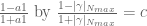


 , we could also use the optimal replacement.
we could optimally also replace
We then want
Using
we then require
Hence for example if
7 May, 2018 at 7:47 am
Terence Tao
This broadly looks correct to me, but it may be good to have a longer description of what you are doing… for instance are you able to edit the relevant section of the writeup on github? A sketch of the calculations there would be helpful.
7 May, 2018 at 10:36 am
KM
It seems the section to be edited is the placeholder kept for the claims (ii) and (iii) proof in zerofree.tex. I will start working on it.
10 May, 2018 at 12:12 pm
KM
I edited section 8 of the writeup (pg 35 and 36 of the pdf) to include the recursive lower bounds. Some things I realized while rederiving the formulas is that
1) if (1-a1)/(1+a1) is replaced with 1, the lemmabound turns into a triangle inequality bound, so this factor has to be kept less than 1,
2) Also, since there are extra d^y in mollified alpha_n, |bn-an|/|bn+an| is more complex than earlier, so computational verification may be needed to ensure it remains below (1-|gamma_Nmax|)/(1+|gamma_Nmax|)
3) While moving from N to N+1, the terms n = dN+[1,d] also undergo a change, not only DN+[1,D], so that should be accounted for.
Some content is still left to be filled, and the formatting could be improved, but I just wanted to confirm on these changes before going forward.
13 May, 2018 at 7:44 am
Terence Tao
Thanks for this! I will go through this writeup soon (am distracted by some other work at present), but looks good so far.
13 May, 2018 at 10:11 pm
KM
I was checking if there is one formula (even if somewhat messy) for the main numerator in the lemma bound which can be turned into a repeatedly callable function, to handle all scenarios automatically and streamline the calculations in this approach. Will something like this work,
With,


14 May, 2018 at 11:51 am
Terence Tao
I’m starting to read through your notes. I am wondering how you get the lower bound on in terms of
  , because the quantities
  (and also the denominator
  vary with
  . In principle these quantities should be generally decreasing in N, but we can’t say for certain because of the oscillations in the weights
  .
.
(Also, strictly speaking all the lower bounds for or
or  need to be multiplied by a factor of
  , which is not relevant insofar as keeping
  away from zero, but which may have some impact on how one can absorb error terms.)
14 May, 2018 at 9:30 pm
KM
On the |moll| part, I was wrongly assuming that it will be less than 1, but since it has terms instead of
  , it is greater than 1 and should be divided. I will make that change.
The way I was thinking about the main terms was that if we calculated the exact lemmabound (eqn 78) for both N and N+1,

 terms comes only through the
  factors.
except potentially when n is in [dN+1,dN+d] for all valid d,
since the dependence on N of the
Also, since
To account for n in [dN+1,dN+d], we could either subtract from the bound the difference or subtract a larger quantity
  to keep the calculations simpler.
Hence, if we choose the right numerators for each n (one of three or four choices), decreases for a given n and N varying.
15 May, 2018 at 9:05 pm
Terence Tao
Ah, I see what you are doing now. This seems to work, in theory at least – how does it perform at the current range of parameters ( , Euler7 mollifier)?
16 May, 2018 at 1:59 am
KM
With t=0.2,y=0.2,N=69098,Euler 7, we get 0.0199 (now dividing by |moll|) which is a bit low if we want to remain above a threshold (eg. 0.02).
This is although not a bottleneck since Rudolph had recently written an optimized script, that computes the exact lemmabound for each N much faster than earlier and helps resolve the bottleneck till about N=200k or so. Using it to cover N till 1.5 million or when dealing with much higher N would still take significant time.
If we use that script to handle N=69098 to 80000 and then use this approach, we get
80000,0.2,0.2,euler5 -> 0.0345
80000,0.2,0.2,euler7 -> 0.0615
which provides a more comfortable buffer.
17 May, 2018 at 3:41 pm
Terence Tao
Hmm, sounds like it’s going to be tough to push beyond then. Given how complicated the argument has become, maybe it is a good time to “declare victory” on the Polymath project and focus on finalising all the various steps required to fully verify that
  ? It sounds like if we step down from Euler 7 to Euler 5, then Euler 3, then Euler 2, we would have a good chance of covering up to say
  in a computationally feasible amount of time.
18 May, 2018 at 1:54 am
KM
The file with exact lemmabounds (euler 5 mollifier) for N in [69098,80000] is kept here, and the one with incremental lemmabounds (euler 5 mollifier) between [80000,1.5 mil] is here (bounds shown for N=100K). The first one ran in about 6 hours, while the latter took about an hour. Also sharing a plot of how the latter file looks like visually.
I have also edited section 8 of the writeup accordingly.
Also, Rudolph and I found that it is possible to push X to something like 10^13 (or maybe higher) using the multiple evaluation algorithm for the barrier strip and the recursive approach for the lower bounds (both would take about a day each at this height). But with RH not verified at this height, the results will be conditional and could be treated as follow-on work.
18 May, 2018 at 3:09 am
KM
Also sharing the results of a parallel exercise,
Exact lemmabounds for N=80k to 150k, y=0.2, t=0.2 with Euler 3 mollifier
Exact lemmabounds for N=150k to 250k, y=0.2, t=0.2 with Euler 2 mollifier
These took around a day each. The second one is currently on hold.
8 May, 2018 at 8:08 am
Anonymous
In the writeup, third line from the end of page 41, the variation of the argument of on the imaginary axis is actually zero (not merely
  ) since
  is positive on the imaginary axis (as clearly seen from its defining integral).
 (instead of
  ).
).
Also in this line, it seems that (in the first portion of the rectangle upper edge) it should be
8 May, 2018 at 11:11 pm
Anonymous
In the results wiki page (zero-free regions), the last two lines should be dated “May 1, 2018” instead of 2017 :) As of today, can we claim “Completes proof of \Lambda = 0.22” for the last entry should be or are we still stuck with “This should establish \Lambda = 0.22”?
[Corrected, thanks – T.]
15 May, 2018 at 4:19 am
Sergei Ofitserov
Dear Terence Tao! I take KM signal and count(consider) necessity to express my opinion. Analyse estimates TE41 and LE61,confidently can to say, what this two-sided stair-well(flight), lower part at which wreck condition! For passage at side”+” it is necessary rig up lengthwise girder(s) of Ricci flow. Thanks! Sergei.
20 May, 2018 at 5:34 am
Anonymous
Going back and forth from this “denglish” to Russian and back to English with Google translate this is Sergei’s comment in a “normal” language (I don’t understand more anyway):
Dear Terence Tao! I accept the KM signal and consider (I believe) the need to express my opinion. Analyzing the estimates of TE41 and LE61, we can confidently say that this is a two-way ladder-flight (flight), the lower part, in which there is an emergency condition! To pass from the “+” side, it is necessary to install a longitudinal beam (s) of the Ricci flow. Thanks! Sergei.
20 May, 2018 at 6:56 am
Anonymous
In the write-up paper, there is a typo in Theorem 3.3, point (iii):
$X\leq x \geq X$ should be $X \leq x \leq X$.
[Fixed, thanks – T.]
21 May, 2018 at 7:01 am
Anonymous
Dear Terry,
If you now return to Twin prime conjecture with the strongest solution to attack over H=246,I think every one is surely amusing.Many night I think Twin prime actually ties the best minds in the world.Twin prime makes every one lots of time.I very annoy this.Terry you quick up!Not it make you very old.If I am an expert mathematician,I break it
21 May, 2018 at 10:45 am
KM
In the eighth thread there was a discussion (https://terrytao.wordpress.com/2018/04/17/polymath15-eighth-thread-going-below-0-28/#comment-496959) whether expanding in the multi evaluation algorithm for the barrier was beneficial.
At the time, I had not expanded this term, and calculated the stored sums for each t step separately, since the computation time at x near 6*10^10 was reasonable. However, the stored sum calculation becomes a relative bottleneck at x near 10^13 or higher.
By incurring a larger overhead at the start where stored sums are calculated for each term in the Taylor expansion of (upto a large number of terms like 40 or 50 to maintain the same accuracy as earlier), we do see a significant benefit. Testing near x=6*10^10,y=0.2,t=0.2 resulted in an 8x reduction in time (from 2 hours to about 15 minutes).
21 May, 2018 at 12:29 pm
Anonymous
Is it possible to reduce the number of terms (while maintaining the required accuracy) by replacing the Taylor series with a suitable truncated series of its Chebyshev polynomial expansion (for a better uniform approximation over appropriate intervals with fewer terms.)
21 May, 2018 at 12:43 pm
Terence Tao
Looks like the barrier part of the argument is now quite tractable!
I will be rather busy with other things in the next week or two, but plan to return to the writeup and try to clean up Section 8 in particular to try to write down all the different parts of the argument before we forget everything. For instance in the barrier computations we still have to show that the 50-term Taylor expansion actually is as accurate as it looks; I’ll have to think about how best to actually show that rigorously (certainly I don’t want to apply the Leibniz rule 50 times and estimate all the resulting terms!). I am thinking perhaps of using the generalised Cauchy integral formula instead to get a reasonably good estimate (we do have tens of orders of magnitude to spare, so hopefully there should be a relatively painless way to proceed).
3 June, 2018 at 12:23 am
KM
While running the barrier scripts for large X (which were being optimized over the past few weeks), we hit on the above question on how to determine the number of taylorterms to use to ensure a certain approximation accuracy. Just wanted to check if the below argument can work.
3 June, 2018 at 12:32 am
KM
Sorry, a correction in , which should be
  .
.
4 June, 2018 at 9:30 pm
Terence Tao
I’ll take a look at this later today. It looks like you are trying to use some sort of Taylor’s theorem with remainder in two variables, which should be available.
I’m actually giving a talk on the de Bruijn-Newman constant in a few hours here in Bristol ( https://heilbronn.ac.uk/2017/08/08/perspectives-on-the-riemann-hypothesis/ ). I’ll mention our tentative bound and some of the methods used to achieve them.
5 June, 2018 at 8:03 am
Anonymous
Wow. It will be cool to have video recordings of the lectures.
[The lectures were filmed and will presumably be made online at some point – T.]
5 June, 2018 at 8:16 am
KM
Also, I wanted to check about a possibly optimistic approach. Right now the number of summands for the B and A sums in (A+B)/B0 is kept equal at N approx = sqrt(x/4Pi).
Since the |gamma| factor diminishes the A sum as x goes higher, is it possible to shift more of the summands to the A sum so that N_A > N_B, and could this help in reducing the bound further..
6 June, 2018 at 9:17 am
Terence Tao
In principle one could vary the two summation ranges (basically removing some of the terms from one sum and inserting a Poisson summation-transformed version of that sum in the other), but I think the gamma factor
  will remain unchanged; in the writeup we bound this quantity by some power of
  , but really we are bounding it by a power of
  and using
  for convenience.
6 June, 2018 at 4:35 am
KM
Within the barrier multiple evaluation approach, is it possible to use the ‘extra’ work done on a rectangle contour, to have a larger t step size, hence reducing the overall number of rectangles processed?
While processing a rectangle, since minmesh = min_|(A+B)/B0|_(meshpoints) is not known in advance, the mesh gap is taken to be a safe value, g/ddxbound (eg. g=1), instead of minmesh/ddxbound. Once the rectangle is processed and minmesh as expected comes out to be larger than g, the lower bound of |(A+B)/B0| between mesh points seems to be (2*minmesh – g)/2. However, currently in the scripts we assume the lower bound to be minmesh/2 and increment t as t_next = t_curr + (minmesh/2)/ddtbound, instead of the larger allowed one.
Near t=0, minmesh is often high, something like 3.x or 4.x (since the barrier strip was chosen accordingly). Due to the ddtbound being also high near t=0, changing the t_next formula results in a nice speedup.
6 June, 2018 at 9:18 am
Terence Tao
Yes, this should work, one just has to use the d/dy bound instead of the d/dx bound for the vertical sides of the rectangle (and make sure that the mesh includes all the corners of the rectangle).
7 June, 2018 at 9:19 am
KM
Just checked the scripts. We have been including the rectangle corners by always starting a side’s mesh from a corner point. Also in lemma 8.2 of the writeup, ddxbound and ddybound are equal, hence no change in the calculations (although will change the name to ddzbound to refer to both).
9 June, 2018 at 6:51 am
Terence Tao
Ah, right, I had forgotten about the Cauchy-Riemann equations! So there isn’t much additional complication caused by turning a corner in the rectangle mesh.
19 August, 2018 at 2:12 am
goingtoinfinity
Is by any chance a Video of that talk already available? That would be interesting. Thanks! If no, would it be fine to ask the organizers?
6 June, 2018 at 9:49 am
Terence Tao
OK, I think I see what you are trying to do here now. One may possibly have to sum over i,j rather than take max over i,j, but other than that, this bound looks more or less correct. I think it’s not essential at this time to have a completely rigorous error bound, as long as it is in the right ballpark; if you can arrange the parameters so that this putative bound is a couple orders of magnitude better than what is needed, then we can probably go back later and write down an analytic bound for the error term that will suffice (possibly sacrificing some of these orders of magnitude in order to shorten the proof of the bound).
I’ll write some general notes on the wiki soon (after I recover from this very interesting, but exhausting, conference!) on how to estimate multiple sums of the form for various pairs
  , which is basically the general form of the problem being considered here. One minor thing is that the precomputed sums
  can be re-used for both the A/B_0 and B/B_0 expressions.
7 June, 2018 at 3:44 am
Terence Tao
I wrote up some explicit error estimates for Taylor expanding these sorts of sums at the end of http://michaelnielsen.org/polymath1/index.php?title=Estimating_a_sum
10 June, 2018 at 10:32 am
KM
The wiki approach of using the same precomputed sums for both A/B0 and B/B0 by shifting y outside the precomputations worked. At large X, since the precomputations take majority of the time, it allows a decent time reduction overall.
26 May, 2018 at 11:33 am
El proyecto Polymath15 logra reducir la cota superior de la constante de Bruijn-Newman | Ciencia | La Ciencia de la Mula Francis
[…] La cota numérica Λ ≤ 0.48 se confirmó de forma analítica en el sexto hilo [Tao, 18 Mar 2018]. El avance parece parco, pero los proyectos Polymath necesitan un arranque suave para que todos los participantes vayan conociendo las herramientas que se van a usar y vayan aportando ideas relevantes. Todo parecía indicar que se podía ir más allá con el método numérico [Tao, 28 Mar 2018], hasta alcanzar una cota de Λ ≤ 0.28 [Tao, 17 Apr 2018]. El método de la barrera desarrollado para el ataque analítico prometía pequeñas mejoras adicionales, que llegaron hasta Λ ≤ 0.22 [Tao, 04 May 2018]. […]
12 June, 2018 at 1:12 am
Anonymous
It seems that with a given computational complexity bound , it is possible to get
  for some absolute constant
  . Is it possible that there is a similar bound
  for another absolute constant
  ?
?
14 June, 2018 at 7:51 am
Terence Tao
Well, lower bounds on complexity are notoriously hard to establish, even heuristically, unless the problem is so “universal” that it encodes some standard complexity class (e.g. if the problem is NP-hard, Turing-complete, etc.). Given that one is only working with the zeta function here, it is unlikely that there is any universality (though one could, in principle, imagine that if one were to consider a much more general problem involving more general PDEs applied to more general functions, one could eventually obtain some sort of universality. In addition, if RH is ever proven, then the time complexity of evaluating drops to
  . :-)
. :-)
Nevertheless, one can informally get a sense of what capturing as follows. If a zero is of the form
  for some
  ,
,  , then one should heuristically expect it to be attracted towards the real axis by heat flow at speed about
  , because there should be about
  zeroes on the real axis at distance
  from this zero. As such, it should hit the real axis in time
  . As such,
  is roughly speaking the best constant such that the zeroes
  lie in the region
  . This is already known in the regime
  , so establishing an upper bound
  is morally equivalent to establishing a certain zero-free region of diameter about
  . In the absence of any major breakthrough on RH (or on numerical verifications thereof), it thus seems that the time complexity of doing this will also be of the form
  ; one could hope to optimise the constant
  but I think it is unlikely that we can remove the exponential with current technology.
18 June, 2018 at 9:27 pm
Anonymous
Prime quadruplet Law of quantity growth
Natural number /// Prime quadruplet Number /// Ratio of the number to
the former
671088649 /// 20557 /// 1.71222722
1342177289 /// 35848 /// 1.743834217
2684354569 /// 62387 /// 1.740320241
5368709129 /// 109113 /// 1.748970138
10737418249 /// 191356 /// 1.753741534
21474836489 /// 338325 /// 1.768039675
42949672969 /// 599598 /// 1.772254489
85899345929 /// 1065802 /// 1.77752761
prime Law of quantity growth
Natural number /// Prime number /// Ratio of the number to the former
671088649 /// 34832025 /// 1.927837377
1342177289 /// 67237143 /// 1.930325412
2684354569 /// 129949340 /// 1.932701691
5368709129 /// 251437996 /// 1.934892443
10737418249 /// 487025115 /// 1.936959102
21474836489 /// 944293561 /// 1.938901161
42949672969 /// 1832604295 /// 1.940714594
85899345929 /// 3559707892 /// 1.942431272
Conclusion:
With the increase of natural number 1 times, the number of primes has
increased by nearly 1 times, and the number of primes of four births
has increased by nearly 1 tim
19 June, 2018 at 3:32 am
Anonymous
It seems that it is possible, with bounded complexity, to approach arbitrarily close, not only from above (as we now know) but also from below !
 ) that
  (i.e. RH is false!), so one may locate (with bounded complexity) a non-real zero of
  with “arriving time to the real axis” arbitrarily close to
  , and then follow numerically (with sufficient precision) its “trajectory”.
To see that, we may assume (since
12 June, 2018 at 6:53 am
Sylvain JULIEN
If RH is true hence $ latex\Lambda=0 $ this would entail $ latex N>\infty$.
19 June, 2018 at 5:39 am
Anonymous
How to explain this kind of imagination:
The number of primes, the number of twin primes, and the number of four cytoplets in the two intervals are basically equal in the two intervals of the same length in a sufficient number. For example, the number of about 10 billion within the range of 100 million prime number four births, the twin prime prime is basically the same:
For example, four births in the 99-100 prime billion between 1458 and 1512 in 100-100, billion between.
There are extreme examples:
6500000000-6600000000 1600 four twin primes;
6600000000-6700000000 1600 four twin primes;
22600000000-22700000000 1305 four twin primes;
22700000000-22800000000 1305 four twin primes;
24700000000-24800000000 1271 four twin primes;
24800000000-24900000000 1271 four twin primes;
27 June, 2018 at 11:39 am
Nazgand
I noticed https://viterbischool.usc.edu/news/2018/06/mathematician-m-d-solves-one-of-the-greatest-open-problems-in-the-history-of-mathematics/ today and thought I should mention here that the Lindelöf hypothesis is claimed to be proved. https://arxiv.org/abs/1708.06607 I suspect that a proof of the Lindelöf hypothesis may improve bound proofs related to the De Bruijn-Newman constant as they are both related to the Riemann Zeta function.
28 June, 2018 at 6:16 am
Terence Tao
The press release notwithstanding, given the very long history of announced proofs of LH or RH that later turned out to be incorrect, I would wait until some professional confirmation occurs (e.g. publication in a reputable journal) before getting too excited. As for this particular manuscript, I notice two things:
1. The paper you linked to only claims an “approach” to LH, with details to follow in a “companion paper” which is apparently not yet available.
2. Several of the estimates in the linked paper look suspiciously weak in that the available bounds on error terms are significantly larger than the main terms, see e.g. Theorem 4.1 where sums such as appear; the main term
  exhibits cancellation but the error term
  need not if the unspecified
  error has a phase that largely cancels out the phase of
  . As such, the main term is swamped by the worst-case bounds on the error term, which are
  if the
  decay rates are uniform in
  .
. and
and  is a very powerful and convenient tool, but one can make a lot of mistakes if one is not careful. (For instance, it is not true that
  in general, if the sum
  exhibits cancellation and the
  terms in the summands vary with
  ; this is most visible in the case that the sum
  cancels completely to zero. The best that one can say in general is that
  , and even then one needs a little bit of uniformity of the
  errors in
  .)
.)
Asymptotic notation such as
28 June, 2018 at 6:31 am
Terence Tao
I am returning (after some hiatus) to trying to finalise the proof of . Here we are erecting a barrier with parameters
  ,
,  ,
,  , and we need to check the inequality
  both at the barrier and in the asymptotic region
  .
.
In the latest version of the writeup (which should hopefully propagate to the main git repository soon), I computed an upper bound on , which is
  in the barrier region and not much larger than that in the asymptotic region. Hopefully this is well within the margin of error for the barrier computations.
Next, I will try to finish off the case of very large x in which one should be able to proceed without any Euler mollifiers. I presume for the remaining portion of the asymptotic region we would divide into subregions where one uses Euler 3, Euler 5, Euler 7, and maybe also Euler11 mollification, and possibly also the lemma that gives a little improvement exploiting the fact that the coefficients are real, though I’ve lost track a bit on what the current status of these numerics are.
29 June, 2018 at 9:15 pm
KM
The barrier and euler bounds calculations are now being primarily computed using very optimized arb scripts recently built by Rudolph.
For X near 6*10^10, the barrier part completes in just around a minute, and the timings increase by around 3 times for every order of magnitude change in X. So far we have reached X near 10^18 and the winding numbers have turned out to be zero. For each such run, we first select an optimized region (eg. X=10^18+44592) such that min_mesh|(A+B)/B0| starts between 4 and 5 at t=0 and ends near 1.5 at t=tmax, hence the lower bound of |(A+B)/B0| is staying well above the error bounds.
For the euler bounds, we have been using the incremental lemmabound computations, as in section 8 of the writeup. For N in [80000,1.5mil] with euler5 mollifier, the computations again complete in around 3 minutes (the remaining part from N=[69098,80000] was verified using the exact formula (eqn.80)). We have also been able to run this for t=0.13,y=0.2 from N=[28209479,700mil], euler5 mollifier thus conditionally verifying dbn <<=0.15 (also similarly dbn<=0.13 is currently being attempted).
The storedsums for various barrier regions is bing stored here, the winding number summaries for these regions here, and the eulerbounds output here.
While running the eulerbounds for large ranges like N=[28209479,700mil], we also wanted to check whether a analytical triangle bound for large x using mollifiers is possible, as it may significantly reduce the upper end of the verification range, and may help us reach dbn<=0.1 conditionally. For eg. in an approach similar to the Estimating a sum wiki, calculating the mollified triangle bound up to small N0, and bounding the tail sum as
29 June, 2018 at 10:22 pm
KM
Actually, in the last line could also the term be removed, and
  changed from
  to
to  to get somewhat larger bounds?
29 June, 2018 at 10:41 pm
Anonymous
The displayed formula seems to be too long for one line.
3 July, 2018 at 11:12 am
KM
I have updated the writeup with a description at the end of section 7 on how candidate shifts can be searched for, with an example of how the 83952 shift near 6*10^10 was found.
4 July, 2018 at 9:01 am
Terence Tao
Thanks for this! I rewrote it a little bit to try to describe in rather concrete terms how the specific shift of 83952 was found, hopefully it is accurate.
My tentative plan for the paper is to try to write up a proof of with enough detail that each step can be replicated fairly easily (it seems now that the total computer time needed is not too onerous), and then to have a final section with some further conditional results, and here perhaps we do not need to provide as many details.
I’d like to understand the situation with the asymptotic analysis (sticking for now with ). In your previous comment you stopped the numerical verification at
  , is this because the simplest triangle inequality bound ((79) in the latest version of the writeup) works at this point (and presumably then also at all later points)? It certainly is possible that by inserting mollifiers in the analytic part of the argument one could also cover some of the region
  with a relatively small amount of numerical effort. But I remember Rudolph had some method involving testing some mesh of N first (e.g. multiples of 100) and using some rather crude bounds on the amount of fluctuation between mesh points that seemed to be rather quick here, are you already using this for
  near
near  ?
?
5 July, 2018 at 2:05 am
Terence Tao
Ah, I think I understand the distinction between and
and  now… it seems that the triangle inequality bound works for
  for
for  (I’ve just adjusted the writeup to include this calculation), but you are working now also with smaller values of
  and the triangle inequality bound is weaker here and is now only available for this much larger value of
  . So for the original purpose of bounding
  by 0.22 we don’t need anything fancier than the triangle bound for the asymptotic analysis, but you would like an improved bound for the asymptotic analysis to go below this value (conditionally on a numerical verification of RH). I’ll take a look to see if there is some reasonably clean estimate analogous to Lemma 1 in “estimating a sum” on the wiki that can handle mollifiers.
6 July, 2018 at 6:27 am
Terence Tao
I did some calculations how the triangle inequality gets modified under an Euler2 mollifier and actually the calculations are relatively clean, see
http://michaelnielsen.org/polymath1/index.php?title=Estimating_a_sum#Euler2_mollifier_in_the_toy_model
This may already reduce the threshold significantly for the values of t,y that you are working with currently.
5 July, 2018 at 9:53 am
KM
Thanks. Also, just wanted to check that given results by Conrey and others that atleast 40%+ zeta zeroes are on the critical line, is it possible to adapt such results to prove for example that atleast 95% of Ht zeroes are real at t=0.21, and can such probabilistic results help constrain things further?
Also, in the first thread you had mentioned that analyzing clusters of zeroes may help better control the dynamics of zeroes. Could probabilistic results help here as well, since a large fraction of the total ‘mass’ would be known to be away from the remaining zeroes, especially from the potentially far-off ones closer to y=1?
5 July, 2018 at 10:10 am
KM
Sorry, I forgot that at t > 0, the number of complex zeroes is finite, so the fraction will always be 1.
7 July, 2018 at 11:02 pm
KM
Thanks. We were using (t=0.13,y=0.2) and using the modified bound, the threshold reduces by 10 times to 70 million (2-(LHS in criterion) = 0.119 with N0=200k).
Also, I was trying out symbolic integration of n^(bln(n)-a). While it does not give a closed form expression, we get a formula in terms of the erfi function, which is commonly available in many tools.

(verified in wolframalpha here, which could provide a sharper tail bound. Can this be used to lower the range further?
8 July, 2018 at 8:13 am
Terence Tao
Sure, one could try using this bound, say for the un-mollified sum in Lemma 1 of http://michaelnielsen.org/polymath1/index.php?title=Estimating_a_sum, using the first inequality in the proof of that lemma rather than the lemma itself and using the erfi formula to evaluate that integral exactly, rather than estimating it as was done in the lemma, and see if it gives significantly superior numerical performance. One thing it should do is make the bound rather insensitive to the choice of N_0, as the integral test should be a pretty sharp bound.
9 July, 2018 at 5:05 am
KM
Using the exact integral indeed reduces the N0 required significantly. The bound is close to its optimal value even at N0 as low as 100 and the change is marginal after N0 around 1000. The bound for (N=30mil,y=0.2,t=0.13,moll 2) is around 0.0582, so the required N_max has dropped further.
Also, using the integral for the tail term in the mollifier criterion instead of the majorizing operation at the end leads to a small but still decent impact (the bound above changes to 0.0685).
To use the ‘spare capacity’ of N=700 mil, (t,y)=(0.11,0.2) can instead be used (bound=0.233)..(although Rudolph recently already covered this (t,y) by running the bounds till N=20 billion, which suggests the capacity available is much higher).
13 July, 2018 at 10:45 am
rudolph01
During the last couple of weeks, KM and I have been progressing the numerical work on the “Barrier approach”. Along the way we did develop and exchange some visual manifestations of the insights we gained. These visuals are now bundled into a single overview deck that can be found here (in pdf and powerpoint):
Visuals
The information is by no means complete and we plan to continuously update it. Hence open to feedback on errors, ommisions or desired improvements.
As the table at the end of the deck illustrates, we have come as far as verifying the numerics for , i.e. a potential
  that is conditional on the RH being verified up to
  . Recently, a bottleneck for computing the Eulerbounds at higher
  was removed (through a much sharper euler2 version of the Triangle bound) and we are now exploring parallel processing techniques (multi-core threading and/or cloud clustering) to ‘attack’ the required Barrier-computations at
  and
and  .
.
In ‘parallel’ to this, we have started work on gathering some statistics on the behaviours of the real and complex zeros below (i.e. the ‘gaseous’ state).
17 July, 2018 at 3:24 pm
Terence Tao
Thanks for this! The visuals are very nice and we should incorporate some of them into the writeup at some point.
I am currently on vacation, but will return next week and hope to update the writeup and the wiki to reflect these developments.
15 July, 2018 at 6:22 am
Anonymous
A very minor remark: the link to the (pdf version of the) visual guide contained in the linked page (which is to say in the file README.md) is broken and should be updated. Keep up the great work!
15 August, 2018 at 5:07 am
KM
We have managed to create a grid computing setup (based on BOINC) for the time consuming steps like stored sums, lemmabounds, etc. at anthgrid.com/dbnupperbound. The framework is quite flexible and can also be adapted to newer computational steps that may come up later.
Instructions on how to install Boinc and run the project’s tasks are kept here.
Currently, we are computing the storedsums matrix for X near 10^19 cell by cell.
It will be great to understand how we can improve the setup further and also use it for related problems.
15 August, 2018 at 5:45 pm
Terence Tao
Wow, that’s impressive! I’m recovering from knee surgery right now, but I’ll try to get around to looking at this more carefully when I can.
16 August, 2018 at 12:37 am
Anonymous
The best starting point should be this thread: github.com/km-git-acc/dbn_upper_bound/issues/81
17 August, 2018 at 7:38 am
rudolph01
In parallel to the work on speeding up the numerical computations (through multi-threading the scripts and using grid computing), we also explored the behaviour of the zeros at more negative . The two tools we currently have available for this domain are the unbounded Ht_integral (eq. 35 in the writeup):
and the well-known effective (A+B-C)/B0 approximation formula.
For more more negative , the trajectories of the real zeros appear to be less chaotic than expected. This is illustrated in the plot below.
Graph of real zeros up to t=-800
Obviously we are keen to explore what happens below and when the ‘real zeros steadily marching south-east’ will collide. The plot was generated using the Ht_integral, however the root finding gets quite unstable at more negative
  and/or larger
  . What could help here is to have a normaliser similar to
  . Also, since the bounded version of the Ht_integral is not valid for negative
  , could it be adopted to cover this domain as well (this would give a more predictable outcome)?
For smaller (up to 1) and
  (up to -2), both functions work properly and their outcomes are close enough. However, the ABC_eff function starts to quickly deviate from the integral at larger
  and/or more negative
  (thereby ruling out the option to use B0 as a normaliser for the Ht_integral). On the other hand, the ABC_eff approximation evaluates very fast compared to the Ht_integral, so is there a viable way to expand its validity towards larger
  and
and  ?
?
P.S. . Since it used the ABC_eff formula, the data cannot be trusted. So far, haven’t been able to reproduce this chart with the Ht_integral. I’ll share the graph anyway, since the emerging patterns are still quite interesting (but could of course also be an artefact of the diverging ABC_eff formula).
Also managed to produce a graph on the behaviour of the complex zeros at negative
Graph of complex zeros up to x=1000
Does theory actually predict a positive relation between and the suprema of
  at a certain significantly negative
  ?
?
17 August, 2018 at 7:44 am
rudolph01
The link to the first picture seems to be broken. Here it is again:
https://drive.google.com/open?id=1fQbCcnhrl7VrBaNMDZSgMt8rPB8pE75J
17 August, 2018 at 1:13 pm
rudolph01
We encountered two potentially contradicting statements about the validity of the Ht_integral for negative . In the derivation of the integral in the write-up, culminating in eq. 35, there is an explicit condition on
  needing to be positive. However, in this comment from April:
it is observed that using negative is also valid (but only in the unbounded version of the third approach integral). The previous post is written assuming the latter interpretation is the correct one, but grateful for a confirmation.
17 August, 2018 at 7:03 pm
Terence Tao
Yes, this formula is valid for negative t also; this is equation (15) of https://arxiv.org/pdf/1801.05914.pdf .
18 August, 2018 at 12:51 pm
Terence Tao
Very interesting! I am not sure whether one can produce good asymptotics for extremely negative values of t such as -800. One can already see trouble in the ABC approximation when t becomes very negative, in that the tail of the A and B sums start to dominate the main term in the sum, also I think the C term will also become quite large in comparison with say B_0, in contrast with small or positive values of t where C is a relatively small term. It might be interesting to plot things like |C/B_0| or |(A+B+C)/B_0| versus the accuracy of the ABC approximation. If the ABC approximation only starts failing when C/B_0 gets large then what it probably means is that all the lower order terms in the Riemann-Siegel expansion now become important. At which point it seems unlikely that we will get a clean asymptotic…
18 August, 2018 at 12:38 pm
Anonymous
This is comments to the references:
– [1]: “Pages 9951009” –> “995–1009”
– [3]: “pp. 609–630” –> “609–630”
– [10]: comma before page numbers
– [16], [18], [24]: Titles should be in italic
– [19]: Maybe link to the arXiv version
– [21]: “pp. 23–41” –> “23–41”
[Updated, thanks. I am using the style where only article titles are italicised, with book titles remaining in Roman font. -T.]
29 August, 2018 at 12:47 pm
Anonymous
Hmmm! Now I can’t find the link to the article anymore. Could you please post the link here?
[The most recent version of the writeup is at https://github.com/km-git-acc/dbn_upper_bound/blob/master/Writeup/debruijn.pdf – T.]
30 August, 2018 at 6:59 am
Anonymous
Thanks for the link.
Some more comments to the references:
– [1]: Remove “Pages”.
– [3]: Remove “pp.”.
– [11]: Remove “pp.”.
– [21] Remove “pp.”.
[Changed, thanks -T.]
26 August, 2018 at 7:43 am
goingtoinfinity
There is a talk by Terence Tao on the Newman-conjecture, also mentioning this polymath project: https://www.youtube.com/watch?v=t908N5gUZA0 (polymath is mentioned at 47.00 and in the discussion)
28 August, 2018 at 4:52 pm
Doug Stoll
Would it possible for T to post a link to the presentation for downloading? Great presentation – now I get it – this whole approach.
Thanks
28 August, 2018 at 8:13 pm
Terence Tao
I’ve uploaded the slides here.
29 August, 2018 at 3:02 am
Anonymous
In page 19, the first lower bound (by Newman) is from 1976 (not 1950).
[Thanks, this will be updated in the next revision of the slides. -T]
29 August, 2018 at 7:32 pm
Yeisson Alexis Acevedo
Question for academic community:
Best Regard, Tao and community
Hi!
I am a Yeisson Acevedo, currently I am
master student in applied mathematics at the Eafit University (Colombia),
I am interested in number theory and I would like to ask you a question that has to do with my object of study that I do not know if it is relevant or not to publish a possible paper, and i would like to ask the favor if you give me your opinions about the next questions:
1) is there a Mersenne Prime such that $M_p = k^2+1$ for some Integer k?
2) Is there a Mersenne prime who is at the same time Germain’s prime?
3) Is there a Mersenne prime who is at the same time Fermat’s prime?
4) Is there a Mersenne prime who is at the same time Wagstaff prime?
5) Is there a Mersenne prime who is at the same time Wodall prime?
6) Is it possible to estimate if around a Mersenne prime there are close primes? That is to say, is Mp +- 2 a prime number?, is Mp +- 4 a prime number?
We want to know if they are important or not in the academic field of number theory and please excuse us for making them spend their time. Thank you.
Pdt: For us, from here in Colombia, the results shared and commented in this blog have been very useful to think about several application problems that go hand in hand with the theory of numbers, although it is not our object of direct study if we use many of your results, so thank you very much for everything.
Knowledge is built in community.
29 August, 2018 at 11:21 pm
Anonymous
It is easy to show that the number 3 is the only solution to your third question.
30 August, 2018 at 4:27 pm
Yeisson Alexis Acevedo
Thank you, you are right … I forgot to write that my questions are for prime numbers greater than or equal to 7 … Thank you
30 August, 2018 at 7:59 am
Anonymous
This is definitely a wrong place to ask these questions. Why don’t you try for example http://mathoverflow.net/ ?
Btw. first question is equivalent to asking if 2^(m-1)-1 = k^2/2, which is the same as asking if there is a Mersenne prime which is even. The only prime which is even is 2, and that is not a Mersenne prime.
30 August, 2018 at 4:22 pm
Yeisson Alexis Acevedo
Thanks for the link, but change 2^p-1 for 2^(m-1)-1 have the problem that “m” must be even but when you solve the system 2^(m-1)-1 = k^2/2 have 2^m-1=k^2+1 which precisely does not refer to a prime number of mersenne since “m” is even….
Again thank you very much for the link, I will also ask there, but still my question remains open … thanks.
3 September, 2018 at 11:35 am
Anonymous
debruijn.tex: There is no need to load the amsmath package; the mathtools package is an extension of amsmath.