Polymath15, eighth thread: going below 0.28

17 April, 2018 in math.NT | Tags: Polymath15

This is the eighth “research” thread of the Polymath15 project to upper bound the de Bruijn-Newman constant ${\Lambda}$ , continuing this post. Discussion of the project of a non-research nature can continue for now in the existing proposal thread. Progress will be summarised at this Polymath wiki page.

Significant progress has been made since the last update; by implementing the “barrier” method to establish zero free regions for $H_t$ by leveraging the extensive existing numerical verification of the Riemann hypothesis (which establishes zero free regions for $H_0$ ), we have been able to improve our upper bound on $\Lambda$ from 0.48 to 0.28. Furthermore, there appears to be a bit of further room to improve the bounds further by tweaking the parameters $t_0, y_0, X$ used in the argument (we are currently using $t_0=0.2, y_0 = 0.4, X = 5 \times 10^9$ ); the most recent idea is to try to use exponential sum estimates to improve the bounds on the derivative of the approximation to $H_t$ that is used in the barrier method, which currently is the most computationally intensive step of the argument.

114 comments

Comments feed for this article

17 April, 2018 at 3:52 pm

Terence Tao

I have reorganised the writeup a bit to try to put the most interesting results in the introduction. Also I have written down a bound for both the x,y and t derivatives of the quantity $A^{eff}+B^{eff}/B^{eff}_0$ , which in the writeup is now called $f_t(x+iy)$ . These should presumably be useful in the barrier part of the argument. I like KM’s idea of using some exponential sum estimates to do even better; the estimates in the paper of Cheng and Graham aren’t too fearsome, and it may be that all one needs to do is combine them with summation by parts to obtain reasonable estimates. The net savings could potentially be on the order of $x^{1/4 - 1/6} = x^{1/12}$ which could be significant at the scales we are considering (in principle we can place our barrier as far out as $x = 6 \times 10^{10}$ ). I’ll take a look at it.

UPDATE: there is also some followup work to the Cheng-Graham paper by various authors which may also have some useable estimates in this regard.

18 April, 2018 at 8:35 am

Anonymous

citizen scientists don’t have mathscinet

18 April, 2018 at 9:34 am

Anonymous

See e.g. the recent paper by Platt and Trudgian

Click to access 1402.3953.pdf

18 April, 2018 at 8:45 am

It seems the t/4 factor in the ddt bound formula should be 1/4. Also, I was facing a authentication wall with the mathscinet link, so tried Google Scholar instead (link), which provides links to many of the followup papers.

[Corrected, thanks – T.]

21 April, 2018 at 5:47 am

Bill Bauer

There may be sign error in the denominator of definition (16), γ. It currently reads

(16) γ(x+iy) := Mₜ(t,(1-y+i*x)/2)/Mₜ(t,(1+y-i*x)/2)

It should, perhaps, read

(16) γ(x+iy) := Mₜ(t,(1-y+i*x)/2)/Mₜ(t,(1+y+i*x)/2)

The mean value theorem, used in the proof of Proposition 6.6 (estimates) suggests that log|Mₜ(t,(σ+i*x)/2)| should be a function of σ only which it would not be if the signs of ix were different in numerator and denominator.

Apologies if I’m missing something obvious. As far as I’ve checked computationally, the inequality seems to be true in either case.

21 April, 2018 at 7:08 am

Terence Tao

The holomorphic function $M_t$ is real on the real axis and so obeys the reflection equation $M_t(\frac{1+y-ix}{2}) = \overline{M_t(\frac{1+y+ix}{2})}$ , so if one takes absolute values, the sign of the $ix$ term becomes irrelevant. I’ll add a line of explanation in the proof of Prop 6.6 to emphasise this.

21 April, 2018 at 10:23 am

William Bauer

Thank you. Wish I’d seen that.

17 April, 2018 at 5:10 pm

anonymous

This is a question which is possibly a bit orthogonal to the main developments of this polymath, but may be able to be answered relatively easily using the insights that the contributors have gained. Is clear how far one can extend to other similar functions the result of Ki, Kim and Lee, that all but finitely many zeros of $H_t(z)$ lie on the real line for any $t > 0$ ? I’m thinking of a result along the lines of de Bruijn’s that applies generically to functions with zeros trapped in a certain strip, with the added condition that zeros become more dense away from the origin.

For instance is there a pathological example of an entire function $G(x+iy)$ (with rapidly decaying and even Fourier transform) with all zeroes in some strip $\{|y| \leq c\}$ , $G_t(z)$ still has infinitely many zeros off the real line? (One could even to make the question more precise suppose $G(z)$ even satisfies a Riemann- von Mangoldt formula with the same sort of error term as the Riemann xi-function.)

17 April, 2018 at 7:49 pm

Terence Tao

Well, here is a simple example: the functions $G_t(z) := e^t \cos z + c$ , for some constant $c>0$ , has all zeroes in a strip that become all real at time $\log c$ , but has infinitely many zeroes off the line before then (the function is $2\pi$ -periodic). But this function doesn’t obey a Riemann von Mangoldt formula.

For a typical function obeying Riemann von Mangoldt, a complex zero above the real axis of real part $T$ would be expected to be attracted to the real axis at a velocity comparable to the $\log T$ nearby zeroes, at least half of which will be at or below the real axis. So within time $1/log T$ one would expect such a zero to hit the real axis, suggesting that there are only finitely many non-real zeroes after any finite amount of time. But there could be some exceptional initial configurations of zeroes which somehow “defy gravity” – maybe “pulling each other up by their bootstraps” and stay above the real line for an unusually long period of time. I don’t know how to construct these, but on the other hand I can’t rule such a scenario out either – they seem somewhat inconsistent with physical intuition such as conservation of centre of mass, but I have not been able to make such intuition rigorous.

17 April, 2018 at 11:53 pm

Anonymous

It seems important to classify (e.g. by Cartan’s equivalence method) all the invariants of the zeros ODE dynamics – to get more information and bounds for this dynamics.

18 April, 2018 at 7:49 am

Terence Tao

I’m not sure that there will be many invariants – this is a heat flow (with a very noticeable “arrow of time”) rather than a Hamiltonian flow. Since such flows tend to converge to an equilibrium state at infinity, it’s very hard to have any invariants (as they would have to match the value of the invariant at the equilibrium state). For such flows it is monotone (or approximately monotone) quantities, rather than invariant quantities, that tend to be more useful (such quantities played a key role in my paper with Brad, for instance). But there’s not really a systematic way (a la Cartan) to find monotone quantities (we found the ones we had by reasoning in analogy with quantities that were useful for a similar-looking flow, Dyson Brownian motion).

22 April, 2018 at 6:20 am

Raphael

Sounds a bit like there should be something like an entropy.

22 April, 2018 at 7:12 am

Raphael

I mean for the one the local entropy gain directly follows from the PDE, on the other hand side one could look at particular “subsystems”. I don’t know if the zeros can be interpreted meaningful as subsystems but in any case “phase change”s like what you suggest in your interpretation are nicely traceable with the entropy. Especially there is the interpretation of entropy as the number of degrees of freedom. In that sense if a zero can be complex or exclusively real directly goes into the entropy (like by a factor of two per particle). Just a loose thought.

17 April, 2018 at 8:19 pm

Nazgand

It occurs me that another way to attack the problem is to use a fixed $x=x_0$ and calculate a mesh barrier over the variables $y,t$ as $t$ varies from the verified upper bound of the de Bruijn-Newman constant, $t_1$ to a target upper bound, $t_0$ and as $y$ varies from 0 to an upper bound of the maximum possible $y$ for the current $t,x$ . This mesh will take care of any zeroes coming from horizontal infinity.Then one can follow some zero, $z(t)$ greater than $x_0$ (at both $t_1,t_0$ through the reverse heat dynamics, and verify that the same number of zeroes exist on the real line up to $z(t)$ . I am assuming that zeroes on the real line are able to join together then exit the real line as $t$ decreases, but if this is shown to be impossible for some $t_0$ close enough to $t_1$ , then only the mesh calculation is required, not the counting of real zeroes.

The current method is working, yet someone may find this idea a useful starting point, as this method nicely recycles previous upper bounds of the constant. This sort of elementary idea is the only thing I see which I can submit that may help, given my shallow understanding of the project.

18 April, 2018 at 7:51 am

Terence Tao

It’s a nice idea to try to move backwards in time from the previous best known bound of $\Lambda$ rather than move forward in time from $t=0$ (which is our current approach that leverages numerical RH). The problem though is that when one moves backwards in time, the real zeroes become very “volatile” – it’s very hard to prevent them from colliding and then moving off the real axis (this basically would require one to somehow exclude “Lehmer pairs” at these values of t. One could potentially do so if one knew that the zeroes were all real at some earlier value of t, but this leads to circular-looking arguments, where one needs to lower the bound on $\Lambda$ in order to lower the bound on $\Lambda$ ).

18 April, 2018 at 3:25 pm

Nazgand

I do not understand what part of my argument is circular, as it is merely another way of verifying that the rectangular region of possible non-real zeroes of $H_{t_0}$ has no non-real zeroes. This is the same rectangular region of possible non-real zeroes the current method uses for fixed $t=t_0$.

If the zeroes are conserved expect for zeroes appearing from horizontal infinity and no zeroes pass through the barrier at $x=x_0$ then counting the number of real zeroes up to $z(t)$ for both $H_{t_0}(z)$ and $H_{t_0}(z)$ and verifying equality implies the rectangle is free of non-real zeroes. If zeroes collide and exit the real line, then the counts of real zeroes will not match.

Is your concern that multiple real zeroes near each other may be miscounted, and that avoiding such miscounts would be costly computation-wise? Much research has been done on counting real zeroes of $H_0(z)$, and applying similar methods to $H_t(z)$ is likely possible.

The idea that the counting of real zeroes might be skip-able is fluffy speculation based on the fact that one world only need to avoid colliding real zeroes for zeroes less than $z(t)$.
Without such a shortcut, counting real zeroes can be expensive for large $x_0$, yet the current method likely uses more computation to lower the bound to $t_0$ because a barrier mesh needs to be calculated which has width $x_0$, leaving only the cost of the mesh at $x=x_0$ to consider, which may be cheaper than the current mesh calculation required.

18 April, 2018 at 4:10 pm

Terence Tao

If one is willing to try to count real zeroes of $H_t$ up to some large threshold $X$ , then this approach could work in principle, but the time complexity of this is likely to scale like $O(X^{3/2})$ at best (to scan each unit interval for zeroes takes about $O(X^{1/2})$ time assuming that the Odlyzko-Schonhage algorithm can be adapted for $H_t$ ). We already had a somewhat similar scan in previous arguments using the argument principle for a rectangular region above the real axis, and even with the additional convergence afforded by having $y$ equal to 0.4 rather than 0, it took a while to reach $X = 10^6$ or so. In contrast, the barrier method only has to scan a single unit interval $[X,X+1]$ (albeit for multiple values of $t$ , which is an issue), and we’ve been able to make it work for $X$ up to $10^9$ so far.

The circularity I was referring to would arise if one wanted to somehow avoid the computationally intensive process of counting real zeroes up to $X$ . In order to do this one would have to somehow exclude the possibility that say $H_{t_0}$ has a Lehmer pair up to this height, as such a pair would make the count of real zeroes very sensitive to the value of $t$ . Given that real zeroes repel each other, the non-existence of Lehmer pairs at $t_0$ is morally equivalent to $H_t$ having real zeroes (up to scale $X$ , at least) for some $t < t_0$ . Actually, now that I write this, I see that this is weaker than requiring one to already possess the bound $\Lambda < t_0$ , since one could still have zeroes off the real axis near horizontal infinity. So there need not be a circularity here. Still, I don't see a way to force the absence of Lehmer pairs without either a scan of length $X$ (and time complexity something like $O(X^{3/2})$ or a barrier method (outsourcing the length $X$ scan to the existing literature on numerical verification of RH).

17 April, 2018 at 10:19 pm

pisoir

Dear prof. Tao,
I have been watching carefully your (fast) progress on this problem and from my point of view I am confused about several of your comments.

To me it seems that you are aiming for $\Lambda \leq 1/4$ , but from the progress made so far, I have the feeling that this is a rather “artificially” picked bound and if you wanted you could push it even further. Also you mention several times the numerical complexity of the problem, but according to the fast results by KM, Rudolph and others, this also does not seem to be a problem at the moment.
So my question is, are you aiming at some specific value of $\Lambda$ and then close the project, because it could then go on forever (pushing the $\Lambda$ by meaningless 0.01 each month) or you will try to push it as far as you can until you really hit the fundamental border of this method? Is there such border and what could that value be (can it go down to e.g. $\Lambda \leq 0.001$ )?
Thanks.

18 April, 2018 at 5:20 am

goingtoinfinity

“by meaningless 0.01 each month” – that would be rather surprising in july 2020.

18 April, 2018 at 7:57 am

Terence Tao

I view the bound on $\Lambda$ as a nice proxy for progress on understanding the behaviour of the $H_t$ , but one should not identify this proxy too strongly with progress itself (cf. Goodhart’s law). Already, the existing efforts to improve the lower bound on $\Lambda$ have revealed a number of useful new results and insights about $H_t$ , such as an efficient Riemann-Siegel type approximation to $H_t$ for large values of x, an efficient integral representation to $H_t$ for small and medium values of x, a “barrier” technique to create large zero free regions for $H_t$ (assuming a corresponding zero free region for $H_0$ ), and an essentially complete understanding of the zeroes of $H_t$ at very large values of x ( $x \geq \exp(C/t)$ ). Hopefully as we keep pushing, more such results and observations will follow. If such results start drying up, and the bound on $\Lambda$ slowly improves from month to month purely from application of ever increasing amounts of computer time, then that would indicate to me that the project has come close to its natural endpoint and it would be a good time to declare victory and write up the results.

18 April, 2018 at 3:54 am

Anonymous

For a given measure of computational complexity (or “effort”), an interesting optimization problem is to find the optimal pair $(t_0, y_0)$ which minimize the bound $t_0 + y_0^2 / 2$ subject to a given computational complexity constraint.

18 April, 2018 at 8:05 am

Terence Tao

It might be worth resurrecting the toy approximation

$\displaystyle \frac{A^{toy} + B^{toy}}{B^{toy}_0} = \sum_{n=1}^N \frac{1}{n^{\frac{1+y-ix}{2}+\frac{t}{4} \log \frac{N^2}{n} - \frac{\pi i t}{8}}} + e^{i\theta} N^{-y} \sum_{n=1}^N \frac{1}{n^{\frac{1-y+ix}{2}+\frac{t}{4} \log \frac{N^2}{n} + \frac{\pi i t}{8}}}$

for this purpose, where $N = \lfloor \sqrt{x/4\pi} \rfloor$ and $\theta = (\frac{x}{2} + \frac{\pi t}{8}) \log \frac{x}{4\pi} - \frac{x}{2} - \frac{\pi}{4}$ (see this page of wiki). For the purposes of locating the most efficient choice of $(t_0,y_0,X)$ parameters that are still computationally feasible, we can just pretend that $H_t / B^{toy}_0$ is exactly equal to this toy approximation (thus totally ignoring $Error_1,Error_2,Error_3$ errors, and also replacing the somewhat messy $\alpha$ factors by a simplified version). Once we locate the most promising choice, we can then return to the more accurate approximation $A^{eff} + B^{eff} / B^{eff}_0$ and combine it with upper bounds on $Error_1, Error_2, Error_3$ .

18 April, 2018 at 8:16 am

Terence Tao

With regards to this toy problem at least, it seems like some version of the Odlyzko–Schönhage algorithm may be computationally efficient in the barrier verification step where we will have to evaluate $A^{toy}+B^{toy}/B^{toy}_0(t, x+iy)$ for many mesh points of $(t,x,y)$ (but with $x$ in a fixed unit interval $[X, X+1]$ . The first basic idea of this algorithm is to transform this problem by performing an FFT in the x variable, so that one is now evaluating things like

$\sum_{m=1}^M \frac{A^{toy}+B^{toy}}{B^{toy}_0}( t, X + \frac{m}{M} + iy ) e^{2\pi i mk/M} \quad (1)$

for $k=1,\dots,M$ , where $m$ is a mesh size parameter. The point is that this FFT interacts nicely with the $n^{\pm ix/2}$ factors in the toy approximation to give a sum which is substantially less oscillatory, and which can be approximated fairly accurately by dividing up the sum into blocks and using a Taylor expansion on each block, which can allow one to reuse a lot of calculations as $k$ varies (basically reducing the time complexity of evaluating (1) for all values of k from the naive cost of $O(M^2)$ to something much smaller like $O(M \log M)$ ; also one should be able to reuse many of these calculations when one varies t and y as well, leading to further time complexity savings). One still has to do a FFT at the end, but this is apparently a very fast step and is definitely not the bottleneck. I’ll have to read up on the algorithm to figure out how to adapt it to this toy problem at least. (In our language, the algorithm is generally formulated to compute the sum $\sum_{n=1}^N \frac{1}{n^{\frac{1+ix}{2}}}$ for many values of $x \in [X,X+1]$ simultaneously.)

18 April, 2018 at 8:01 am

Anonymous

Is it possible to derive (perhaps by using exponential sums estimates) for each given positive $t_0, y_0$ an explicit numerical threshold $X(t_0, y_0)$ with the property that $H_{t_0}(x + i y) \neq 0$ whenever $0 < y \leq y_0$ and $x \geq X(t_0, y_0)$ ?

If so, then (clearly) $X(t_0, y_0)$ should decrease with increasing $y_0$ and therefore is preferable over the currently used $X(t_0, 0) = \exp (C/t_0)$ (i.e. with $y_0 = 0$ ) in the barrier method.

Since $X(t_0, y_0)$ may also be used as a kind of "computational complexity measure", Is it possible that $X(t_0, t_0^{1/2})$ (i.e. with $y_0 = t_0^{1/2}$ ) grows much slower than $X(t_0, 0)$ as $t_0 \to 0$ ? (while still giving the bound $1.5 t_0$ – comparable to the bound $t_0$ with $y_0 = 0$ .)

18 April, 2018 at 8:34 am

Terence Tao

In general it gets harder and harder to keep $H_t(x+iy)$ away from zero as y gets smaller – after all, we expect to have a lot of zeroes $H_t(x+iy)=0$ with $y=0$ . The two methods that we have been able to use to actually improve the bound on $\Lambda$ only require keeping $H_t(x+iy)$ away from zero for $y \geq y_0$ , where $y_0$ is something moderately large like 0.4. While we do have some capability to probe near $y=0$ (in particular, in the asymptotics section there are some arguments using Jensen’s formula and the argument principle that make all the zeroes real beyond $\exp(C/t)$ for some large absolute constant $C$ ), I think numerically this sort of control will be much weaker for computationally feasible values of $x$ than the control we can get for large values of $y$ . (One can already see this when considering the main term 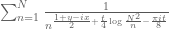$\sum_{n=1}^N \frac{1}{n^{\frac{1+y-ix}{2} + \frac{t}{4} \log \frac{N^2}{n} - \frac{\pi i t}{8}}}$ of the toy expansion, in which the role of increasing y in improving the convergence of the sum is quite visible.)

18 April, 2018 at 10:31 am

Anonymous

Correction: in the above required property of $X(t_0, y_0)$ , it should be $y \geq y_0$ (instead of $0 < y \leq y_0$ ).

18 April, 2018 at 1:29 pm

Mark

I haven’t been following this project at all, so apologies for the basic question which is perhaps covered in the discussion elsewhere:

But how much of a dictionary relating \Lambda and zero-free regions do we have? The kinds of things that I mean by a “dictionary” might be:
1) If we could prove there is a zero free strip, does that imply anything about \Lambda?
2) If there were only a single pair of off critical line zeros, can we convert this into a value of \Lambda depending on their coordinates?
3) If we knew \lambda < 10^{-1000}, would that give us any usable zero-free region?

More philosophically, I'm curious why in the "de Bruijn-Newman score system" it feels like real progress on the Riemann-Hypothesis is being made while (and I'd love to be wrong here) it doesn't seem that the ideas being applied (numerical verification, etc) are circumventing any of the obstructions to progress in other the other "score systems" (zero-free regions, etc.)

18 April, 2018 at 2:02 pm

Anonymous

wait, are you saying when we reach $\Lambda \le 1/4$ then we’re *not* really half way to proving rieman hypothesis???

18 April, 2018 at 3:57 pm

Terence Tao

The basic theorem here is due to de Bruijn (Theorem 13 of https://pure.tue.nl/ws/files/1769368/597490.pdf ), which in our language says that if $H_{t_0}$ has all zeroes in the strip $|y| \leq y_0$ , then one has the bound $\Lambda \leq t_0 + \frac{1}{2} y_0^2$ . For instance, the proof of the prime number theorem gives this for $t_0 = 0, y_0=1$ , yielding de Bruijn’s bound $\Lambda \leq 1/2$ . So zero free regions for zeta or for $H_{t_0}$ can give bounds on $\Lambda$ . However we don’t seem to have any converse implication, beyond the tautological assertion that $H_t$ has all real zeroes for all $t \geq \Lambda$ . Having a really good upper bound on $\Lambda$ such as $\Lambda \leq 10^{-10}$ may rule out certain scenarios very far from RH (such as having a single pair of zeroes far from the critical line, and also relatively far from all other zeroes) but it would be tricky to convert it into a clean statement about, say, a zero-free region. So perhaps one reason why we can make progress on bounding $\Lambda$ , but not on other approximations to RH, is that the implications only go in one direction.

If somehow we could show that RH is true with a single exceptional complex pair of zeroes, it should be possible to track that zero numerically with high precision and get a precise value on $\Lambda$ , assuming that pair was within reach of numerical verification. Otherwise one could use de Bruijn’s theorem to obtain a bound, though it would not be optimal.

18 April, 2018 at 4:42 pm

Terence Tao

I have a sort of statistical mechanics intuition for the zeroes of $H_t$ which may help clarify the situation. A bit like the three classical states of matter, the zeroes of $H_t$ seem to take one of three forms: “gaseous”, in which the zeroes are complex, “liquid”, in which the zeroes are real but not evenly spaced, and “solid” in which the zeroes are real and evenly spaced. (This should somehow correspond to the $\beta<0$ , $\beta=2$ , and $\beta=\infty$ limiting cases of beta ensembles, but I do not know how to make this intuition at all rigorous.) At time zero $t = 0$ , the zeroes are some mixture of liquid and gaseous, and the RH (as well as supporting hypotheses such as GUE) asserts that it is purely liquid. At positive time, the situation is similar to $t=0$ in a region of the form $|x| \leq \exp(C/t)$ (though perhaps slightly "cooler", with some of the gas becoming liquid), but for $|x| \geq \exp(C/t)$ the zeroes have "frozen" into a solid state, so in particular there is only a finite amount of gas or liquid at positive time. As time advances, more of the gas (if any) condenses into liquid, and the liquid freezes into solid; by time $\Lambda$ , all the gas is gone, and pretty soon after that it all looks solid. In the reverse direction, we know that at any negative time, there is at least some gas.

With this perspective, the reason why it is easier to make progress on $\Lambda$ than on other metrics towards RH is that we are dealing with an object $H_t$ which is already almost completely "solidified" into something well understood: the mysterious liquid and gaseous phases that make the Riemann zeta function so hard to understand only have a finite (albeit large) spatial extent, and so can be treated numerically, at least in principle.

19 April, 2018 at 9:48 am

Rudolph01

I really like the analogy and it makes me wonder what then is causing the phase-transitions between solid, liquid and gaseous. Here’s a free-flow of some thoughts, going backwards in time and assuming RH.

From solid to liquid:
When we were starting to ‘mollify’ the toy-model, I recall the surprise to still see a vestige of a partial Euler product even at $t=0.4$ . So, with $t \rightarrow 0$ , we could reason that this partial Euler product needs to incrementally grow back towards its well-known infinite version at $t=0$ . When we follow the trajectories of the real zeros going back in (positive) time, they will feel an increasing competitive pressure w.r.t. their neighbouring zeros to occupy the available space to encode all the required information about the primes. This increasingly ‘heated battle’ for available locations when $t \rightarrow 0$ , does ‘bend’ their trajectories and determines the angle and the velocity by which they hit the line $t=0$ . Statistics will force some angles to become very small and these will then induce a Lehmer-pair. So, it could be the increasing need to encode an infinite amount of information about the primes, that turns up the ‘heat/pressure’ and moves the statistical ensembles of real lines from solid to liquid.

Liquid to gaseous:
Is there a need for an extra ‘heat/pressure’ source to explain why a perfect liquid at $t=0$ slowly turns into a gaseous state? I don’t think so, since the ‘heat is already on’ at the line $t=0$ and all the collision courses for the real zeros have been determined. The real zeros ‘plunge’ as it were into the domain below $t =0$ ((like particles flying into a bubble chamber) and their angles and velocities determine at which $-t$ a collision will occur. So, no extra heat source is needed and only the ‘backward heat flow’ logic is required to explain the trajectories below $t=0$ .

Of course the key question is why the collisions of real zeros can only occur below $t=0$ . What is it that suddenly allows liquidized real zeros to collide and send off some gaseous complex zeros in $-t$ -steps? What has really changed below $t=0$ ? I looked at potential ‘switches’ in our formulae like the $\sqrt{t}$ in the 3rd-approach integral, but that doesn’t lead us anywhere. The only thing that I can think of that is really different for $t$ below $0$ , is that there is no longer extra ‘heat/pressure’ being added (since the infinite Euler product has been completed at $t=0$ ). It seems therefore that somehow this incremental ‘heat/pressure’ build-up when $t \rightarrow 0$ , is at the same time also the prohibiting force for real zeros to collide. And this feels like a circular reasoning and probably brings us back again to the duality between the primes and the non-trivial zeros…

19 April, 2018 at 10:33 am

Rudolph01

Couldn’t resist producing an illustrative visual of the analogy.. The trajectory of the real zeros is based on real data, I manually added fictitious data to reflect the trajectory of the complex zeros.

18 April, 2018 at 6:04 pm

Terence Tao

Consider the model problem of evaluating

$\displaystyle \sum_{n=1}^N \frac{1}{n^{\frac{1+y-ix}{2}+ \frac{t}{4} \log \frac{N^2}{n} - \pi it/8}}$

for multiple choices of $x,y,t$ , with $x$ in an interval $[X,X+1]$ . If one does this naively, $M$ different evaluations of this sum would require about $MN$ operations. There is a relatively cheap way to cut down this computation (at the cost of a bit of accuracy) without any FFT, simply by performing a Taylor expansion on intervals. Namely, pick some $H$ between $1$ and $N$ and split the sum into about $N/H$ subsums of the form

$\displaystyle \sum_{n=n_0+1}^{n_0+H} \frac{1}{n^{\frac{1+y-ix}{2}+ \frac{t}{4} \log \frac{N^2}{n} - \pi it/8}}$

(actually it is slightly more advantageous to use summation ranges centred around $n_0$ , rather than to the right of $n_0$ , but let us ignore this for the time being). Writing $n = n_0 + h$ , and also $x = X + \theta$ , we can write this expression as

$\displaystyle \frac{1}{n_0^{\frac{1+y-i\theta}{2}+ \frac{t}{4} \log \frac{N^2}{n_0} - \pi it/8}} \sum_{h=1}^H (n_0+h)^{iX/2} \times$
$\displaystyle \times \exp( (-\frac{1+y-i\theta}{2} + \pi it/8 - \frac{t}{4} \log \frac{N^2}{n_0^2}) \log(1+\frac{h}{n_0}) + \frac{t}{2} \log^2(1+\frac{h}{n_0}) ).$

For $H$ small compared to $n_0$ , we can hope to Taylor approximate $\log(1+\frac{h}{n_0}) \approx \frac{h}{n_0}$ , leading eventually to the first-order approximation

$\displaystyle \frac{1}{n_0^{\frac{1+y-i\theta}{2}+ \frac{t}{4} \log \frac{N^2}{n_0} - \pi it/8}} \times$
$\displaystyle \times ( \sum_{h=1}^H (n_0+h)^{iX/2} + (-\frac{1+y-i\theta}{2} + \pi i t/8 - \frac{t}{4} \log \frac{N^2}{n_0^2}) \sum_{h=1}^H (n_0+h)^{iX/2} \frac{h}{n_0}).$

The point of this is that if one wants to evaluate this subsum at $M$ different choices of $(\theta,y,t)$ , one only needs $O(M+H)$ evaluations rather than $O(MH)$ because one only needs to compute the sums $\sum_{h=1}^H (n_0+h)^{iX/2}$ and $\sum_{h=1}^H (n_0+h)^{iX/2} \frac{h}{n_0}$ once rather than $M$ times, as they can be reused across the evaluations. Putting together the $N/H$ subsums, this cuts down the time complexity from $O(NM)$ to $O(\frac{NM}{H} + N)$ . One can also Taylor expand to higher order than first-order which allows one to take $H$ larger at the cost of worsening the implied constant in the $O()$ notation. There is some optimisation to be done but this should already lead to some speedup, possibly as much an order of magnitude or so.

19 April, 2018 at 3:41 am

Anonymous

The “first sum” can be represented as
$\zeta (-i X/2, n_0 +1) - \zeta (-i X/2, n_0 + H +1)$
where $zeta (s, a)$ is Hurwitz Zeta function
https://dlmf.nist.gov/25.11
https://en.wikipedia.org/wiki/Hurwitz_zeta_function

The “second sum” is

$(1/n_0) \sum_{n=n_0 +1} ^{n_0 + H} n^{1+ i X/2}$ – “first sum”

which has a similar representation in terms of Hurwitz Zeta function.

Efficient algorithms for Hurwitz Zeta and related functions and oscillatory series are given in Vepstas’ paper

Click to access 0702243.pdf

20 April, 2018 at 10:12 pm

With H=10 and near X=6*10^10, I have been able to get a speedup of 3x to 4x (although more should be realizable) which increases gradually as M increases.

To keep H away from n0, the first few terms in the sum are computed exactly (currently I used first 1000 terms for this part), and approximate estimates are used for the remainder sum. Divergence from actual is near the 7th or 8 decimal point.

21 April, 2018 at 7:24 am

Terence Tao

That’s promising! Do you have a rough estimate as to what M (the number of $(x,y,t)$ values that need to be evaluated) might be for the barrier computation, based on what happened back at $t=0.2, y=0.4, X = 5 \times 10^9$ ? The main boost to speed should come in the large M regime. Also, if one uses symmetric sums $\sum_{n=n_0-H/2+1}^{n_0+H/2}$ rather than asymmetric sums $\sum_{n=n_0+1}^{n_0+H}$ then the error term should be a bit smaller (by a factor of 4 or so), which should allow one to make H a bit bigger for a given level of accuracy. One could also Taylor expand to second order rather than first to obtain significantly more accuracy, though the formulae get messier when one does so which may counteract the speedup. (Presumably one should start storing quantities such as $\frac{1+y-i\theta}{2} + \frac{t}{4} \log \frac{N^2}{n_0} - \frac{\pi i t}{8}$ that appear multiple times in such formulae so that one does not compute them multiple times, though this is probably not the bottleneck in the computation.)

21 April, 2018 at 10:57 am

I checked the ddx bound at N=69098, y=0.3, t=0 and it comes out to around 1000. If we choose a strip where |(A+B)/B0| seems to stay high (for eg. X = 6*10^10 + 2099 + [0,1] looks good in this respect) and assume it will stay above 1, M too seems to be around 1000. At N=69098, y=0.3, t=0.2, the ddx bound drops significantly to around 5.

The earlier script was refined so that it is now 6x to 7x faster than direct summation. I will check how varying H, number of Taylor terms and optimizing further can result in further speedup.

22 April, 2018 at 1:18 am

Writing the Taylor expansion of the exponential in a more general form, it seems possible to improve the accuracy to as much as desired. Also, retaining and not approximating the two log factors does not incur a noticeable cost (storing the repeatedly occuring quantities kind of offsets it) while improving accuracy a bit. For eg. at H=10 and 4 Taylor terms, accuracy improves to 12 digits, and with 10 terms improves to 28 digits taking only 1.5x more time).

Near X=6*10^10, with H=50 and 4 Taylor terms, I was able to get estimates for 1000 points in around 1.5 minutes with 9 digit accuracy, which was a 20x speedup vs direct estimation.

22 April, 2018 at 7:12 am

Terence Tao

Sounds good! Could you expand a little on which log factors you found it better to not approximate? [EDIT: I guess you mean doing a Taylor expansion in $\delta := \log(1+\frac{h}{n_0})$ rather than in $h$ ? I can see that that would be slightly more efficient.]

For some very minor accuracy improvements, one could work in a range $x \in X + [-1/2,1/2]$ rather than $x \in X + [0,1]$ ; also, since we have some lower bound $y_0$ on $y$ , we can write $y = y_0 + z$ (say) and pull out a factor of $(n_0+h)^{\frac{-1-y_0+iX}{2}}$ rather than $(n_0+h)^{iX/2}$ in order to replace the $\frac{1+y-i\theta}{2}$ factors with the slightly smaller $\frac{z-i\theta}{2}$ . This should improve the accuracy of the Taylor expansions by a factor of two or so with each term in the expansion, especially in the most important case when t is close to 0 and y close to y_0.

22 April, 2018 at 8:11 am

I will try these out for more improvements. Also, it seems replacing log(N) +- i*Pi/8 with arrays of alpha(s) or alpha(1-s) values to get a close match to the exact (A+B)/B0 estimates also works. I was able to run the script for an entire rectangle (4000 points) in around 6 minutes.

22 April, 2018 at 8:43 am

For the n0 sums, I calculated and stored sums of the form
$\sum_{h=1}^H (n_0+h)^{\pm iX/2} \exp((t/4)\log^2(1+\frac{h}{n_0}))\log^m(1+\frac{h}{n_0})$
where m ranges from 0 to T-1 and T is the number of desired Taylor terms which can be passed to the function to approximate the larger exponential.
Replacing $\exp((t/4)\log^2(1+\frac{h}{n_0}))$ with $1+\frac {t h^2}{4 n_{0}^2}$ in the sums did not result in a noticeable speed difference overall, so I kept it in its original form.

22 April, 2018 at 1:09 pm

Terence Tao

Thanks for the clarification. I guess that while we will need to evaluate at thousands of values of $x$ (and perhaps hundreds of values of $y$ as well), we won’t need as many values of $t$ to evaluate (and the evaluation becomes much faster as $t$ increases), so there is not much advantage to remove the t-dependence in the inner sums, so it makes sense to keep factors such as $\exp( (t/4) \log^2(1+h/n_0))$ unexpanded. In that case one can simplify the expressions a bit by writing

$\displaystyle \frac{1}{n^{\frac{1+y-ix}{2} + \frac{t}{4} \log \frac{N^2}{n} - \frac{\pi i t}{8}}}$

for $x = X + \theta$ , $y = y_0 + z$ , $n = n_0 + h$ as

$\displaystyle \frac{n_0^{\frac{-z+i\theta}{2}}}{(n_0+h)^{\frac{1+y_0-iX}{2} + \frac{t}{4} \log \frac{N^2}{n_0+h} - \frac{\pi i t}{8}}} \exp( \frac{-z+i\theta}{2} \log(1 + \frac{h}{n_0}) )$

and use Taylor expansion of the exponential to decouple the $h$ variable from the $\theta,z$ variables.

It seems like we may have a choice of approximations to use: the $A^{eff}+B^{eff}$ approximation is our most accurate one (especially if we also insert the $C^{eff}$ correction), but the toy approximation $A^{toy} + B^{toy}$ may have acceptable accuracy at the $x \sim 6 \times 10^{10}$ level and will be easier to work with (for instance I’d be likely to make fewer typos with computing d/dt type expressions in the latter : ). Do you have a sense of how complicated it would be to adapt these Taylor expansion techniques to the sums that show up in the $A^{eff}+B^{eff} / B^{eff}_0$ expansion? If it is too messy or slow then it may be worth focusing efforts on establishing a barrier for $A^{toy} + B^{toy} / B^{toy}_0$ instead and reworking some of the writeup to provide effective estimates for the error of the toy approximation rather than the effective one.

23 April, 2018 at 10:25 am

I have to still try out the y0+z form of the estimate, but in the earlier one it seems instead of calculating
$\frac{1}{n_0^{\frac{t}{4}\log n_0 - P_{n_0,\theta,toy}}} \sum\limits_{m=0}^{T-1} \frac{P_{n_0,\theta,toy}^m S_{n_0,H,m}}{m!}$
$\textrm{with } P_{n_0,\theta,toy} = -\frac{1+y-i\theta}{2} + \pi it/8 - \frac{t}{2} \log \frac{N}{n_0}$
we calculate
$\frac{1}{n_0^{\frac{t}{4}\log n_0 - P_{n_0,\theta,eff}}} \sum\limits_{m=0}^{T-1} \frac{P_{n_0,\theta,eff}^m S_{n_0,H,m}}{m!}$
$\textrm{with } P_{n_0,\theta,eff} = -\frac{1+y-i\theta}{2} - \frac{t}{2} \alpha(\frac{1+y-i(X+\theta)}{2}) + \frac{t}{2}\log n_0$
and $S_{n_0,H,m}$ the sum in the earlier comment, and using an array of $A_{0}^{eff}/B_{0}^{eff}$ instead of $\frac{1}{N^y}$ (also with appropriate adjustments for the A sum and when y varies instead of x),
we can switch from approximations of the toy model to approximations of the effective model, with some additional overhead (however the parigp library atleast does well and keeps the overhead small).

Also, on the discrepancy between the toy and effective estimates, at X=6*10^10, y=0.3, t=0.2 $A^{toy}/A_{0}^{toy} \approx A^{eff}/A_{0}^{eff} \textrm{ and } B^{toy}/B_{0}^{toy} \approx B^{eff}/B_{0}^{eff}$ with divergence around the 6th or 7th decimal, but $A_{0}^{eff}/B_{0}^{eff} \textrm{ and } \frac{1}{N^y}$ are different.

Some sample values:

theta,[(A+B)/B0]_toy, [(A+B)/B0]_eff, [(A+B)/B0]_toy_with_exact_gamma
0.0, 0.844 + 0.192i, 0.802 + 0.228i, 0.802 + 0.228i
0.5, 0.812 + 0.165i, 0.792 + 0.199i, 0.792 + 0.199i
1.0, 0.787 + 0.128i, 0.782 + 0.150i, 0.782 + 0.150i

the difference being only due to the different gamma factor.

23 April, 2018 at 6:31 pm

Terence Tao

OK, thanks for this. It sounds like the numerics will be able to handle the effective approximation without too much additional difficulty, so this looks to be a better path than trying to fix up the toy approximation to become more accurate (though this could probably be done by using a more careful Taylor expansion of gamma). It will be a bit messier to rigorously control the error in the Taylor expansion for the effective approximation than the toy approximation, but there should be a lot of room in the error bounds (it looks like we could in fact lose several orders of magnitude in the error bounds if we Taylor expand to a reasonably high order) so hopefully we could use relatively crude estimates to handle this.

24 April, 2018 at 10:25 am

After making the three changes (y0+z, [X-1/2,X+1/2], and symmetric n0 sums), accuracy seems to improve by 2-3 digits.

25 April, 2018 at 6:35 am

Terence Tao

Excellent! Hopefully we can trade in surplus accuracy for speed later by increasing the H parameter.

Since we have a fixed value of $X$ , and the barrier computation is largely insensitive to the choice of $t$ (in particular, a barrier computation for large t can be re-used as is for any smaller value of t, or for any larger value of $y$ ), it seems the next thing to do is to figure out what the smallest value of $y$ is for which the barrier computation is feasible. Given that, the main numerical task remaining would be to find the best values of $y,t$ above this $y$ threshold for which the Euler product calculations work at $X$ and above; combining that with analytic error estimates and some treatment of the case of very large $x$ will then presumably yield a bound for $\Lambda$ which is close to the limits of our methods.

25 April, 2018 at 9:10 am

Anonymous

If t0 is small enough and X is carefully chosen, would it be possible to have y0=0 for the barrier computation?

25 April, 2018 at 10:26 am

Rudolph01

Intriguing question, Anonymous!

Just a few thoughts on this, I might be incorrect. If $y_0=0$ would be in reach of numerical verification to achieve a ‘fully closed’ barrier, isn’t then the issue that at $y_0=0$ we will find real zeros when $t$ goes from $0 \cdots t_0$ ? Of course, we could carefully pick a $X$ and avoid a known real zero at $t=0$ , however we also have to account for all other real zeros that are ‘marching up leftwards’ and could travel through the barrier at $y_0=0$ .

However, would we actually still require a ‘double’ barrier when the barrier reaches all the way to $y_0=0$ (i.e. no complex zeros can fly from right to left around the $y_0$ -corner anymore)? If indeed not, then maybe the way out is to just count all real zeros on the line $y_0=0$ and $t=0 \cdots t_0$ and subtract them from the total winding number found when scanning the entire barrier ‘rectangle’?

25 April, 2018 at 2:05 pm

Terence Tao

Yes, it seems theoretically possible to achieve this, though it may require a stupendous amount of numerical accuracy to actually pull off. It will probably help to have $X$ vary a bit in time, moving to the left to stay away from zeroes. If we can find a continuously varying function $X(t)$ such that for all $0 \leq t \leq t_0$ , there are no zeroes in the line segment $\{ X(t)+iy: 0 \leq y \leq 1 \}$ (including at the real endpoint $X(t)$ ), and all zeroes to the left of $X(0)$ are known to be real at time $t=0$ , then this already implies that all zeroes to the left of $X(t)$ are real at times $0 \leq t \leq t_0$ , since no complex zeroes can penetrate the barrier, and no real zeroes can become complex at later times. But this would require a very accurate approximation of $H_t(x+iy)$ near $X(t)$ , since no matter where one places $X(t)$ one is going to be quite close to one of the real zeroes. In particular the $A^{eff}+B^{eff}$ type approximations we have been using may be inadequate for this, one may need to use $A^{eff}+B^{eff}-C^{eff}$ or an even higher order expansion. (My understanding is that similar higher order Riemann-Siegel expansions were what were already used in existing numerical verifications of RH. It may be that this is a task better suited for some experts in numerical RH verification, rather than our current Polymath group.)

25 April, 2018 at 5:53 pm

Anonymous

> some experts in numerical RH verification, rather than our current Polymath group

it’s about 20 degrees cooler in this shade

26 April, 2018 at 11:19 am

At N=69098 and t=0.2, we are getting these lower bounds

y, Bound type, Bound value, verification required upto approx N
0.20, Euler 5 Lemma, 0.0699, 1.5 million
0.25, Euler 3 Triangle, 0.0270, 900k

The first one currently looks quite slow to compute and also requires a large verification range. The second one looks feasible.

27 April, 2018 at 2:24 pm

Terence Tao

OK, so I guess we can try to target $t=2, y=0.25$ then (which would give $\Lambda \leq 0.23125$ ). It all hinges on whether we can still compute enough of a mesh for the barrier though…

26 April, 2018 at 11:39 am

Anonymous

Since the bound is $\Lambda \leq t_0 + y_0^2 /2$ , it seems that it does not make sense for a given $t_0$ to expand much effort to reduce $y_0^2 / 2$ much below $t_0$ .

28 April, 2018 at 2:25 am

Anonymous

Another possible strategy is to reduce slightly $t_0$ from 0.2 to 0.15 (say), and compensate for the added computational complexity by increasing(!) slightly $y_0$ from 0.25 to 0.3 (say), with the resulting bound $\Lambda \leq 0.15 + 0.3^2/2 = 0.195$ – (better even than the limiting choice $y_0 = 0$ for $t_0 = 0.2$ ).

The idea behind this optimization of $t_0$ and $y_0$ is that if $y_0^2 /2$ is sufficiently smaller than $t_0$ , it seems better to reduce slightly $t_0$ and increase(!) slightly $y_0$ to keep reasonable computational complexity rather than the strategy of reducing both $t_0$ and $y_0$ .

28 April, 2018 at 6:43 am

I was kind of intrigued by the n0 sums so have been working to optimize it further. Firstly, just like X, after making y0+z symmetric so that the anchor point is (1+y0)/2, it seems the accuracy is more consistent along the rectangle.

Eliminating any head or tail exact partial sums, making H=N, and increasing the number of Taylor terms to something like 30 or 50 (with 50 terms, we seem to get above 25 digit accuracy), the same rectangle (4000 mesh points) can be computed under 10 seconds (from 6 min earlier).

It seems this way the entire barrier strip can be covered within a day. Working now on combining this with the adaptive t mesh.

29 April, 2018 at 1:29 pm

Terence Tao

Wow, that is surprisingly good performance! It actually surprises me that H can be taken as large as N, I would have expected the Taylor series expansion to start becoming very poorly convergent at this scale, but I guess the point is that by taking a huge number of Taylor terms one can compensate for this. An analogy would be computing $\exp(x)$ by Taylor expansion (where for our purposes $x$ could be something on the order of $\frac{1}{2}\log N$ after the various symmetrising tricks). Normally one would only want to perform Taylor expansion for x in a range like [-1,1], but if one is willing to take 50 terms then I guess things are good up to something like [-10,10] (the Taylor series $\sum_n x^n/n!$ for $\exp(x)$ peaks at around $n=x$ ) and so perhaps one can indeed treat expressions that are of magnitude $\frac{1}{2} \log N$ or so for our current choice of $N$ .

28 April, 2018 at 8:49 pm

The barrier strip X=6*10^10+2099 + [0,1] (N=69098), y=[0.2,1], t=[0,0.2] was covered (moving forward in t) and the output is kept here and here. The first file gives summary stats for each t in the adaptive t mesh, and the second file gives (A+B)/B0 values for all (x,y,t) mesh points considered. The winding number came out to be zero for each rectangle.

The multieval method with 50 Taylor terms was used to estimate (A+B)/B0 values along each rectangle. The overall computation time for the strip was around 2.5 hours. Since ddt bounds and ddx bounds take time to compute, they were updated only after every 100 rectangles. For each rectangle, the number of mesh points for each side was kept as ceil(ddx bound) (the strip was chosen where minabb = min rectangle mesh |(A+B)/B0| value was expected to be above 1, indicating an allowable step size above 1/(ddx bound)). This overcompensates a bit for the constant x sides since they are a bit shorter. The t jump used was minabb/(2*ddt bound).

29 April, 2018 at 1:51 pm

Terence Tao

That’s great progress! What is the minimum distance of $(A + B)/B_0$ amongst the mesh points? At such large values of $N,x$ , the error terms $E_1,E_2,E_3$ should be essentially negligible in this setting, though now that $y$ and $t$ are a bit lower than what we have dealt with in the past, one may have to be a bit more careful, particularly when $t=0$ . However, there is a tradeoff between t and y that we could potentially exploit: I think it is possible to replace the condition $y \geq y_0$ in the barrier with the slightly weaker $y \geq \sqrt{y_0^2 + 2(t_0-t)} = \sqrt{2(\Lambda-t)}$ , thus one can make the barrier higher at small values of t and only reach $y_0$ at the final time $t_0$ , basically because even if a zero sneaks underneath the elevated barrier at the earlier time it will still be attracted to its complex conjugate and eventually fall down to height $y_0$ or below at time $t_0$ . I haven’t fully checked this claim and having such a moving barrier would also complicate the derivative analysis (one has to compute a total derivative rather than a partial derivative). But it looks like the numerics on the barrier side are now good enough that it is no longer the bottleneck (if I understand your previous comments correctly, the Euler mollifier component of the argument may now be the dominant remaining computation), so maybe this refinement is not needed at this stage.

28 April, 2018 at 8:57 pm

Also forgot to mention that y=[0.2,1] was used since the Euler 5 Lemma bound is positive at N=69098,y=0.2,t=0.2 and maybe there will be a faster way to calculate this up to the required N. Although right now I am finding it too slow, so will start with y=0.25, t=0.2 and the Euler 3 and 2 triangle bounds.

29 April, 2018 at 8:46 am

Rudolph01

Using KM’s latest script, a rerun for the same barrier strip $X=6 \cdot 10^{10}+2099 + [0,1], y=[0.2,1], t=[0,0.2]$ , but now recalculating the ddx and ddt-bounds for each rectangle, completed in 2 hours and 17 minutes. As expected the number of rectangles (or t-steps) to be verified, dropped from $600$ to $440$ .

Here is the output:

Summary per rectangle

Full detail

30 April, 2018 at 6:50 am

At t=0, y=0.2, N=69098, e_A + e_B + e_C,0 is 0.0012, hence not that small. For the t=0 rectangle, the gap between mesh points was taken as around 1/(ddx bound at t=0) for the sides where x varies and 0.8/ddx bound for the sides where y varies (using the ddx terminology for both ddx and ddy).

In this particular strip, the minimum |(A+B)/B0| for the t=0 mesh point set turned out to be around 2.374, and above 1.3 for the all the mesh points in all the rectangles considered. From this it seems that between the mesh points, |(A+B)/B0| here can’t go below about 1.185 for t=0 or below 0.65 for the other rectangles (or maybe a bit larger since the step size along the rectangles was conservative than what a adaptive ddx based mesh would have allowed).

Since t_next was set as t + min_|(A+B)/B0|_t / ddt_bound, it seems |(A+B)/B0| can’t go below 0.325 between the t points, though not sure whether the |f(z)|/2 concept can be applied in the t dimension.

30 April, 2018 at 8:30 am

Terence Tao

It’s interesting that $|A+B|/|B_0|$ is now exceeding 1 at t=0. Is this the reason for selecting $X = 6 \times 10^{10} + 2099 + [0,1]$ ? I would have expected this function to have average size comparable to 1, so the minimum would usually be less than 1.

I think the $|f(z)|/2$ lower bound should work in the t variable as it does in the x or y variables (as long as the quantity $\min|(A+B)/B_0|$ is estimated on the entire contour, and not just on the mesh, so one also needs some control on x and y derivatives). But it does seem that there is plenty of room between $|A+B/B_0|$ and the error terms $e_A+e_B+e_{C,0}$ to accommodate any other errors we have to deal with (e.g. the error term in the 50-term Taylor expansion; I’m not sure how best to control that error yet, but given how small it is compared to everything else presumably we will be able to get away with a quite crude estimate here).

30 April, 2018 at 11:06 am

Yes, this particular X was chosen after some exploration to get large jumps in t. |(A+B)/B0| does seem to have a tendency to jump sharply occasionally near t=0.
For example, I recently accidentally hit upon X=201062000500 (N=126491), y=0.2, t=0, where the estimate is 15.92 (error bound 0.0009). Changing y to 0.1 gives 23.16, and changing y to 0 gives 38.51. It seems local spikes of H_0 do not die down that quickly.

30 April, 2018 at 11:52 am

To accelerate the mollifier bounds calculations (2-b-a), can we use a strategy like this:

Suppose we know the bound at N and it is positive enough and we are trying to reuse it for the bound at N+1. The DN terms each for the A and B parts) for the bounds at N and N+1 are similar except for the (t/2)Re(alpha) factor. Hence we subtract the the extra D terms from the bound at N to get a conservative estimate for that at N+1. Similarly to get the bound at N+2 from that at N+1. The conservative bound slowly decreases towards a postive predetermined threshold and we then update the base N again with the exact bound. Actually it seems this looks quite similar to a N mesh except there are a few calculations for each N.

30 April, 2018 at 5:23 pm

Terence Tao

This looks like it should work. Another variant, which may be a little simpler, is to take the current $(A+B)/B_0$ approximation, which I will call $(A_N+B_N)/B_0$ to make the dependence on $N$ explicit, and approximate it by $(A_{N_0}+B_{N_0})/B_0$ for $N$ in a mesh interval $[N_0,N_0+H)$ . For $H$ small, say $H = 10$ , one can hopefully estimate the error between the two approximations and keep it well under acceptable levels. Then we can apply the Euler mollifier method to $(A_{N_0}+B_{N_0})/B_0$ and bound this for all $x$ in the range with $N_0 \leq N < N_0+H$ . With this approach, one doesn't have to analyse the more complicated sums arising from the Euler mollifications of $A_N+B_N$ .

Also, relating to Euler mollification: the vestige of the Euler product formula $\sum_{n=1}^\infty \frac{1}{n^s} = \prod_p (1 + \frac{1}{p^s} + \frac{1}{p^{2s}} + \dots)$ suggests, heuristically at least, that $H_t(x+iy)$ will be a little larger than usual when the argument of $p^{ix/2}$ is close to zero for small primes $p$ , or equivalently if $\frac{\log p}{4\pi} x$ is close to an integer for (say) $p=2,3,5$ . This heuristic seems to be in good agreement with your choice of $x = 6 \times 10^{10} + 2099$ , where $\frac{\log 2}{4\pi} x$ has fractional part $\approx 0.068$ and $\frac{\log 3}{4\pi} x$ has fractional part $\approx 0.996$ (though things are worse at p=5). It might be that one could use this heuristic to locate some promising further candidate scales x which one could then test numerically to see if they outperform the ones you already found. In particular, a partial Euler product $\prod_{p \leq P} (1 - \frac{1}{p^{\frac{1-ix}{2}}})^{-1}$ for some small value of $P$ (e.g. $P=5$ ) could perhaps serve as a proxy for how large one might expect $H_t(x+iy)$ to be. (Not coincidentally, these factors also show up in the Euler mollification method. One might also work with the more complicated variant 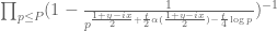$\prod_{p \leq P} (1 - \frac{1}{p^{\frac{1+y-ix}{2}+\frac{t}{2} \alpha(\frac{1+y-ix}{2}) -\frac{t}{4} \log p}})^{-1}$ , though this may not make too much difference especially since we are primarily concerned with $t,y$ near zero. )

1 May, 2018 at 4:54 am

Anonymous

Dirichlet’s theorem on simultaneous Diophantine approximation (which follows from the pigeonhole principle) states that for any sequence of real numbers $\alpha_1, ..., \alpha_n$ , any sequence of consecutive integers $x_1, ... , x_Q$ contains an integer $x$ such that

$|| \alpha_j x || < Q^{-1/n}$ for $j = 1, ... , n$

Where $||x||$ denotes the distance from $x$ to its nearest integer.

Hence (with $\alpha_j := (\log p_j) / (4 \pi)$ ) where $p_j$ denotes the j-th prime, it follows that for a mollifier based on three primes, and $Q = 2100$ , it is possible to find $x$ such that

$||\alpha_j x|| < 2100^{-1/3} = 0.078...$ ( $j=1, 2, 3$ )

1 May, 2018 at 8:37 am

By evaluating sum(||x * alpha_p||) or evaluating the Euler product for a large number of x (for eg. 6*10^10 + n, n the first 100k integers), and sorting to get small sums or large products, we get several candidates where |(A+B)/B0| is greater than 50. It seems this can be turned into a general method to choose a good barrier strip.

Some optimizations which further help are to compute the Euler products for x-0.5,x,x+0.5 and filter for x where all three are high, and to use a larger number of primes. Even with these the whole exercise is quite fast (about 2-3 minutes). Also since min |(A+B)/B0| for a rectangle generally occurs on the y=1 side, it helps to search for candidates using the Euler products at both y=0 and y=1.

Using first 5 primes and the above filters, I could find a candidate X=6*10^10+83952, where the estimate is 72.5 at y=0 and 5.13 at y=1. Running the barrier strip with X+[-0.5,0.5], y=[0.2,1], min |(A+B)/B0| started at 4.32 for the t=0 rectangle (2.374 for the earlier strip), and much fewer t steps were overall needed (280 instead of 440).

2 May, 2018 at 2:36 am

Rudolph01

KM’s idea (outlined a few posts back), for optimizing the ‘mollified’ computations that need to ensure that $H_t$ does not vanish in the range from the Barrier (N=69098) till the point where analytics take over (N=1,500,000), seems to work out very well! Only calculating a small number of incremental terms when moving from N to N+1, dramatically improves speed and indeed results in a slowly declining (hence more conservative) lower bound. We actually found the bound declines so slowly and stayed so far above a full-recomputation-threshold, that we never had to recompute the bound at all throughout the entire range. This implies we only require a full (relatively slow) compute of the first N in the range (i.e. at the Barrier) and this also enables the use of higher mollifiers again (for speed reasons we were considering moving back to $t=0.2,y=0.25$ with Euler 3, but now could easily use $t=0.2,y=0.2$ with Euler 5).

The run for $t=y=0.2, N = 69098...1500000$ , step 1, Euler 5 mollifier, completed in just 60 minutes. Output run. Fields: N, bound.

Here are also the upper error bounds for $t=y=0.2, N = 60000...1510000$ in steps of $50000$ . Fields: $N_0, 3 \times e_B, e_{C,0}, total$ .

If all correct, this would bring us close to a $\Lambda \le 0.22$ :)

2 May, 2018 at 11:23 am

Terence Tao

Great news! It seems like we have all the pieces needed to complete the proof of $\Lambda \leq 0.22$ , I guess one has to check the analytic argument for $N \geq 1.5 \times 10^6$ but perhaps you have done this already. It looks like both of the big computations (the barrier computation and the Euler mollification bound computation) are now quite feasible, but I don’t know whether there is much hope to push $y$ and $t$ much further, at some point I would imagine the Euler mollification bounds will simply fail to prevent zeroes at $N \approx 60000$ at which point we will be stuck (since it is probably not feasible to scan all of this region (as opposed to a narrow barrier) with direct evaluation of $A+B/B$ ).

2 May, 2018 at 12:15 pm

While computing the exact mollifier bounds with Euler 7 and higher looks generally infeasible at these heights, is it possible to use an estimate like this to check whether a bound with a high enough mollifier turns positive. Only the first N terms in the B and A mollified bounds are computed exactly, and the remainder is bounded using the approach in the Estimating a Sum wiki.

$\textrm{For a given mollifier and N}$
$b^{t}_{n/d} = exp((\frac{t}{4})\log^{2}(\frac{n}{d}))$
$= exp((\frac{t}{4})(\log^{2} n - 2 \log n \log d + \log^{2} d))$
$= \frac{b^{t}_{n} b^{t}_{d}}{n^{(t/2)\log d}} < \frac{b^{t}_{n} b^{t}_{d}}{N^{(t/2)\log d}} \textrm{..(for } n > N)$

$\textrm{Hence } |\beta_{n}| = |\sum\limits_{d=1}^{D} 1_{n<=dN} 1_{d|n} \lambda_d b^{t}_{n/d}| < b^{t}_{n} \sum\limits_{d=1}^{D} \frac {b^{t}_{d}|\lambda_d|}{N^{(t/2)\log d}} = C_1 b^{t}_{n}$
$\textrm{and similarly}$
$\textrm{Hence } |\alpha_{n}| < n^y b^{t}_{n} \sum\limits_{d=1}^{D} \frac {b^{t}_{d}|\lambda_d|}{d^y N^{(t/2)\log d}} = C_2 n^y b^{t}_{n}$

$\sum\limits_{n=1}^{DN}\frac{|\beta_{n}|}{n^\sigma} <\approx \sum\limits_{n=1}^{N}\frac{|\beta_{n}|}{n^\sigma} + C_1 TS_{B,N,DN}$
$\sum\limits_{n=1}^{DN}\frac{|\alpha_{n}|}{n^\sigma} <\approx \sum\limits_{n=1}^{N}\frac{|\alpha_{n}|}{n^\sigma} + C_2 TS_{A,N,DN}$
$\textrm{ TS being the tail sum bound from the Estimating a Sum wiki assuming the toy model for the remainder N(D-1) terms}$

2 May, 2018 at 3:08 pm

Terence Tao

Yes, this should work, and also combines well with the strategy of grouping the $N$ into batches $N \in [N_0,N_0+H]$ and trying to prove an Euler bound for an entire batch simultaneously. The tail bound could get rather messy though at Euler7.

3 May, 2018 at 10:39 am

In practice decoupling n and d as above seems to give bounds which are quite different from the exact ones and the gap increases if a higher mollifier is used. Instead of the tail sum bound I also checked the exact value of $\sum\limits_{N+1}^{DN}\frac{b^{t}_{n}}{n^\sigma}$ which too is relatively large, so a bit stuck here.

The error between (A+B)/B_0 and (A+B)/B_0 truncated to N_0 terms is much smaller compared to |(A+B)/B_0| and seems roughly dependent on N_0. For eg. using N_0=60000, the error is around 10^-4.

4 May, 2018 at 2:47 am

It seems the tail sum bound can be replaced with a sharper quantity
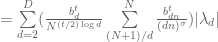
$= \sum\limits_{d=2}^{D}(\frac{b^{t}_{d}}{N^{(t/2)\log d}}\sum\limits_{(N+1)/d}^{N}\frac{b^{t}_{dn}}{(dn)^\sigma}) |\lambda_d|$
$< \sum\limits_{d=2}^{D}(\frac{b^{t}_{d}}{N^{(t/2)\log d}} \max(N^{1-\sigma_B -(t/4) \log N}, (dN)^{1-\sigma_B -(t/4) \log (N/d)}) \frac{\log d}{d}) |\lambda_d|$
and with similar adjustments for the A tail sum

Also, if we then use a weaker mollifier with only prime terms and no interaction terms (for eg. $[\lambda_1,\lambda_2,\lambda_3,\lambda_5,\lambda_7,..]$ ) the gap between the approximate and the actual bound decreases sharply (I think since the terms in the mollified sum all have the same sign), but the bound still becomes more negative as the mollifier is taken higher.
If we assume the tail terms take a trapezoid shape with a curved side instead of a convex shape (which should be the case for $\frac{t}{4}log n < \frac{1 \pm y}{2} + \frac{t}{2}log N$ ) we could use
$\frac {N^{1-\sigma_B -(t/4) \log N} + (dN)^{1-\sigma_B -(t/4) \log (N/d)}}{2}$
instead of the max factor in the tail bound.
With this the bound does improve as we we keep on increasing the mollifier, although atleast with the triangle bound at N=69098 and t=y=0.2, it plateaud at a negative value. Will also now check the behavior for the approximate lemma bound.

4 May, 2018 at 2:49 pm

Terence Tao

Thanks for this. The mollifier calculations seem to be getting quite complicated, we may well be near the limits of what can be done here even if we assume enough computational capacity to evaluate all the mollifier bounds. Do you have a sense of how badly things start breaking down if one tries to decrease t or y any further beyond 0.2? (Maybe one could continue this discussion on the new thread though, this one has become rather full.)

19 April, 2018 at 7:48 am

Sylvain JULIEN

Dear Terry,

Your analogy is interesting and as the physical state of matter is essentially determined by two physical parameters, namely temperature and pressure, it could be useful to define analogues thereof and maybe to show that $ latex \Lambda $ corresponds to the triple point of water, where it can exist under the three states solid liquid and gaseous simultaneously. This would be consistent with the seemingly “critical” nature of this constant.

19 April, 2018 at 7:55 am

Sylvain JULIEN

Perhaps a first step to do so would be to establish theoretically an analogue of the ideal gas relation $ \latex P=nkT $ where $ P $ is the pressure, $ T $ the absolute temperature, k a universal constant and n the number of particles per unit volume. I guess the analogue of the latter would be the number of zeroes in a domain of area 1.

19 April, 2018 at 7:52 pm

Anonymous

How uniform is the ddt bound in lemma 8.2 in the writeup?

20 April, 2018 at 9:24 am

Terence Tao

It holds for all $(x,y,t)$ in the region given by (5).

20 April, 2018 at 10:38 pm

Anonymous

Perhaps “uniform” was the wrong word to use, but I don’t understand how a ddt bound for (x, y, t) helps to establish claim (i) unless the ddt bound applies to an interval, preferably an interval like (X <= x <= X+1, y0 <= y <= 1, t_i <= t <= t_j).

21 April, 2018 at 7:36 am

Terence Tao

Each individual term in the bound is either monotone decreasing or increasing in each of the variables $x, y, t$ , so in a range such as the one you indicate, you can replace the occurrence of each variable by either its lower or its upper bound as appropriate. (In some cases one may need Lemma 5.1(vi) to establish monotonicity of terms such as $\frac{|1+y+ix|}{4\pi} / (x-6)$ in $x$ .)

21 April, 2018 at 12:08 pm

Anonymous

Something strange is going on between gamma and lambda (both lower case) in the writeup. Should the instances of lambda that are not related to mollification be replaced by gamma?

[Yes, this is now fixed – T.]

21 April, 2018 at 2:56 pm

Anonymous

There is a line in the writeup like “log lambda = (t/4)[…]” and later there is a line like “d/dt log gamma = (t/4)[…]”. Should the first line be changed to “log gamma = (t/4)[…]” and the second line be changed to “d/dt log gamma = (1/4)[…]”?

[Yes, this is now fixed – T.]

21 April, 2018 at 3:37 pm

Anonymous

To me it looks like the “log gamma = …” and the “d/dt log gamma = …” lines conflict with each other. In the d/dt log gamma line, should t/4 be replaced by 1/4?

[Ah, I see now. Corrected in latest version – T.]

22 April, 2018 at 7:23 am

Anonymous

In github comments there is still some question about some of the terms in the d/dt bound in lemma 8.2. Specifically the derivation of the (pi/4)*log(n) term in both sums, and why the 2*log(n)/(x-6) term is in the first sum but not the second sum.

22 April, 2018 at 7:56 am

Terence Tao

The second $2 \log n / (x-6)$ was omitted by mistake, I have restored it. As for the first term, I have added an additional line of explanation: because we have

$\displaystyle \alpha( \frac{ 1 \pm y + ix}{2} ) = \frac{1}{2} \log \frac{x}{4\pi} + \frac{\pi i}{4} + O_{\leq}( \frac{4}{x-6} )$

we can conjugate to obtain

$\displaystyle \alpha( \frac{ 1 \pm y - ix}{2} ) = \frac{1}{2} \log \frac{x}{4\pi} - \frac{\pi i}{4} + O_{\leq}( \frac{4}{x-6} ).$

Incidentally, I do not know how to find the github comments you are referring to, do you have a link?

22 April, 2018 at 9:32 am

Anonymous

If I understand the comments in github, the question is about the expression (1/4) log(n) log(x / 4 pi n) + (pi/4) log(n) in the first and second sums of the |d/dt| bound, and whether (pi/4) log(n) could be changed to (pi/8) log(n).

I think the reasoning was that the expression originally comes from (alpha((1 + y – ix)/2)/2) log(n), and that alpha((1 + y – ix)/2) is approximated by (1/2)log(x / 4 pi) – (pi i)/4 + …, so when this is divided by two and multiplied by log(n) and the triangle inequality is applied, it should end up with a (pi/8) log(n) term instead of a (pi/4) log(n) term.

The comment I was referring to is at https://github.com/km-git-acc/dbn_upper_bound/pull/77#issuecomment-383368402. The github for this project is not organized in a normal way.

22 April, 2018 at 12:49 pm

Terence Tao

Thanks for the clarification and the link. KM was correct, there was a typo and one could replace the $\pi/4$ factor here by the $\pi/8$ factor.

Perhaps the best thing to do, as suggested elsewhere by KM, is to replace the $A^{eff}+B^{eff}$ approximation by a very slightly less accurate approximation in which the rather messy $\alpha$ factors are replaced by $\log N \pm i \pi/4$ , making the approximation resemble the $A^{toy}+B^{toy}$ approximation instead. Actually I am tempted to simply _use_ the toy approximation and derive effective error bounds for that approximation; this toy approximation was not so great at the previous values of $x$ we were working with, but with $x$ as large as $6 \times 10^{10}$ it’s actually not that bad. (The error between the two is something of the order of $O( \log x / x )$ , I think.) I guess it should not be too difficult to do some numerical experimentation to get some idea of the discrepancy between $A^{eff}+B^{eff} / B^{eff}_0$ and $A^{toy} + B^{toy} / B^{toy}_0$ ; if the discrepancy is small enough, we can perhaps just use the toy approximation throughout which will make things like the d/dt calculations and Taylor expansion calculations a lot cleaner.

22 April, 2018 at 7:42 am

Anonymous

In the writeup Lemma 8.2 applies to region (5) which includes 0 < t <= 1/2. Do either of the bounds in that lemma apply to t=0? In particular I would like to use the |d/dt| bound at t=0 as an upper bound of |d/dt| on some interval if possible.

22 April, 2018 at 7:58 am

Terence Tao

Yes, $H_t$ varies smoothly in $t$ , so one can extend these bounds to the $t=0$ case.

23 April, 2018 at 7:48 am

Anonymous

Is the change of $arg(H_t(x + i y_0) / B_0(x + i y_0))$ from $x = 0$ to $x = X$ , being only $O(\log X)$ for large $X$ ?
If so, it seems that tracking the argument changes can be done using only(!) $O(\log X)$ values of $x$ .

23 April, 2018 at 6:27 pm

Terence Tao

The ratio $H_t(x+iy) / B_0(x+iy)$ converges to 1 as $x \to \infty$ for any fixed $y>0$ , and should also be quite close to 1 when y is large (e.g. $y=10$ and $x \geq 200$ should suffice). So, assuming no zeroes of $H_t$ for $y \geq y_0$ , the total variation of argument of $H_t(x+iy_0)/B_0(x+iy_0)$ should be bounded from $x=0$ to $x=X$ . But since we don’t actually know in advance that this is a zero free region, one would presumably have to scan the entire range $0 \leq x \leq X$ (or use something like the barrier argument we are currently using) in order to actually compute this variation.

24 April, 2018 at 2:12 am

Anonymous

It seems that you meant “as $x \to \infty$ “. [Corrected, thanks – T.]
Anyway, if the real part of $H_t(x) / B_0$ is positive on an horizontal sub-interval $[x_k + i y, x_{k+1} + i y]$ , the magnitude of its argument increment over this sub-interval should be less than $\pi$ . Is it possible to improve the adaptive mesh used to evaluate the winding number of $H_t / B_0$ around a given rectangle ?

24 April, 2018 at 7:03 am

Terence Tao

Some improvement to previous winding number arguments are presumably possible. But the most extensive calculation we were able to accomplish so far was to scan a region $0 \leq x \leq 1.13 \times 10^6$ at $t = y = 0.4$ . Currently we are taking $t,y$ to be significantly smaller, and $x$ to be as large as $6 \times 10^{10}$ , so many orders of magnitude improvement over the previous state of the art for the argument principle methods would need to be established for these methods to be competitive.

24 April, 2018 at 6:51 am

Anonymous

In page 4 of the paper, in the estimate (sixth line below (24))

$f_t(x + i y) = 1 + O(x^{- t \log 2 / 4})$

Is the constant of the O-term dependent on $t$ (and unbounded as $t \to 0$ )?

27 April, 2018 at 6:23 am

Rudolph01

Just for fun, here is a visual that (almost exactly) captures the trajectories of both the real and the complex zeros into a single 3D-plot for a certain range of $x,y,t$ . For the evaluation of $|H_t(x+yi)|$ I used the third approach integral (the unbounded version).

The real zeros are calculated exactly, however for the complex zeros I used a proxy and stopped scanning when $|H_t(x+yi)| \le 0.03$ for the first time. I normalised $|H_t|$ by simply multiplying it with $10^{28}$ .

I believe the 3D root trajectories look exactly as the theory predicts :)

27 April, 2018 at 6:52 am

Anonymous

This is interesting since one can use this plot by pairing known consecutive real roots of $H_0$ by going backwards in time to see from which double real root of $H_{t_0}$ (for some negative “initial time” $t_0$ ) they “emerge” and what is the value of their common “initial time” $t_0$ .

27 April, 2018 at 9:06 am

Rudolph01

Yes, that is indeed the case. You can make pairs of real roots and find common ‘initial time of birth’. There a snag though about the ‘known consecutive real roots at $H_0$ ‘. Just take a look at the attached 2D frame for $y=0$ , that outlines a wider view of the trajectories of the real roots over time. It immediately becomes clear that pairs of real zeros are not necessarily consecutive (at $H_0$ ) and also that they could have been born out of complex pair collision a ‘long time ago’.

Trajectories of real zeros

27 April, 2018 at 10:34 am

Anonymous

Yes, immediately after their “birth” (from a double zero) they are consecutive, but later a new pair may appear between them.

27 April, 2018 at 1:55 pm

Rudolph01

General theory predicts that all complex zeros of $H_t(x+iy)$ must travel within a ‘hyperbolic tunnel’ $y = \sqrt{1-2t}$ , until they collide with their conjugates.

Using the ‘barrier approach’, we have shown that for $t_0=0.2$ , the rectangle $y=0.4..y_h, x=0 \cdots \infty$ is zero-free, hence $\Lambda \le 0.28$ . In this diagram I tried to visualise this situation. The zero-free rectangle is shown as a red ‘ceiling’ at $t_0$ , where complex zeros can’t travel through (note that I exchanged $y$ and $t$ to obtain the blue hyperbola $t = \frac{1-y^2}{2}$ ). The area directly above the red ceiling (marked in darker green) now also must be free of complex zeros.

I then wondered whether these red ‘ceilings’ also cast down a ‘zero-free shadow’, that further constrains the possible trajectories for the complex zeros below it. My logic would be that $\Lambda \le 0.28$ could be construed from many different $t_0,y_0$ -combinations. E.g. $y_0=0.6,t_0=0.1$ or $y_0=0.74833,t_0=0$ . These combinations are reflected as points on the smaller red-dashed hyperbola, with the greyed areas as the new zero-free regions. Is this reasoning correct?

If this is correct, then an idea could be to use a previously achieved result to further reduce the $y$ -width of a new barrier to be verified (due to a smaller hyperbola). This of course only makes sense when the X-location of the barrier is moved further up in the new calculation, otherwise just lowering $t_0$ would allow full reuse of the already verified barrier.

28 April, 2018 at 3:39 am

Rudolph01

Oops. I suddenly saw where my logic fails. There are indeed many combinations of $y_0,t_0$ that lead to a $\Lambda = 0.28$ , however these combinations are not equivalent. I believe it is still true that a proven zero-free rectangle at $t_0, y=y_0..y_h, x=0 \cdots \infty$ makes all rectangles for combinations $t_0', y_0'$ for the same $\Lambda$ that occur ‘later’ (i.e. $t_0' \ge t_0$ ) also zero-free, however the reverse is clearly not true.

Take for instance the rectangle $t_0=0, y=0.74833..1, x=0 \cdots \infty$ that resides way ‘earlier’ than the proven zero-free rectangle $t_0=0.2, y=0.4..y_h, x=0 \cdots \infty$ . Both yield $\Lambda = 0.28$ , but still zeros could fly through the ‘earlier’ rectangle and collide on the real axis way below $t=0.28$ …

I still believe that there is some sort of a smaller zero-free ‘shade’ just below the proven rectangles. Is this correct?

29 April, 2018 at 1:37 pm

Terence Tao

Nice visual! Unfortunately, while we have a lower bound on the rate at which the furthest zero falls towards the real axis, we don’t have an upper bound (in addition to the attraction that this zero feels to its complex conjugate, it will also be attracted to the infinitely many other zeroes). So I don’t know how to establish a zero free region of the sort you indicate; it could be that a zero stays close to the original de Bruijn bound until just before time $t_0$ , when it decides for some random reason to fall very rapidly towards the real axis. This is a very unlikely scenario, and possibly one that can be eliminated to some extent with a more delicate analysis (based on some sort of statement asserting that if a zero experiences an unusually strong pull towards the real axis at time $t_0$ , then it must also experience unusually strong pulls at some earlier times), but I don’t see a “cheap” way to do so.

3 May, 2018 at 3:54 pm

Anonymous

In the writeup, it seems that in the line below (32), “zero” should be “nonzero at $0$ “.

[Corrected, thanks -T.]

4 May, 2018 at 1:18 pm

Rudolph01

Acknowledging that lowering $t_0$ towards $t_0=0$ or even below it, would make the verification of a zero-free region for $H_{t_0}(x+iy)$ probably exponentially harder, I would like to test a thought that I have outlined in this visual.

There are many $(t_0, y_0), t_0 \le 0$ combinations that would give a $\Lambda=0$ , e.g. $(-0.5,1)$ . I believe the formula for the width of a particular ‘ceiling’ to be verified then is: $\sqrt{1-2t_0}-\sqrt{-2t_0}$ . This would imply that when $t \rightarrow -\infty$ , the ‘ceiling’ width to be verified becomes infinitely small. Is this indeed correct?

Going back in time, there will be a point when the number of complex zeros will stabilise, i.e. the point before which all real zeros have ‘collided’ and no new complex zeros will be ‘generated’ (up to a certain $X$ ). After the collision of two real zeros, the complex zeros will ‘take-off’ from the real line at a guaranteed minimum velocity (there is however no limit on the maximum take-off velocity), hence they will all move steadily away from the real line and travel closer and closer towards the edge of the De Bruijn hyperbola (blue curve in the visual). Could these movements imply that the situation at very large negative $t$ becomes less ‘gaseous’ and sufficiently ‘solid’ again, thereby potentially re-enabling the verification of a zero-free ‘ceiling’?

4 May, 2018 at 2:38 pm

Terence Tao

Our understanding of the zeroes for negative time is rather poor. De Bruijn’s upper bound is only available at times $t \geq 0$ . In my paper with Brad Rodgers, we were not able to get a uniform bound on the imaginary parts of zeroes at negative times; instead we got the weaker bound $y =O( \log(1 + x))$ which is undoubtedly not optimal, but is the best we could manage. One can already see the difficulty in the A+B approximation (it has not been rigorously proven yet that the A+B approximation is accurate in the negative t regime, but I could imagine that this could be done with some effort). This approximation contains terms like $\sum_{n=1}^N \frac{1}{n^{\frac{1+y-ix}{2} + \frac{t}{4} \log \frac{N^2}{n}}}$ . For positive $t$ , the $\frac{t}{4} \log \frac{N^2}{n}$ factor eventually helps with the convergence and makes the $n=1$ term dominate, which is where the “freezing to solid” behavior is coming from. But for negative $t$ , this term now hurts instead of helps, and makes the sum much wilder, particularly at large values of $N$ . So I would expect it should become increasingly “gaseous”, though I don’t have a good intuition on exactly how much so.

4 May, 2018 at 2:23 pm

Polymath15, ninth thread: going below 0.22? | What's new

[…] thread of the Polymath15 project to upper bound the de Bruijn-Newman constant , continuing this post. Discussion of the project of a non-research nature can continue for now in the existing proposal […]

26 May, 2018 at 11:29 am

El proyecto Polymath15 logra reducir la cota superior de la constante de Bruijn-Newman | Ciencia | La Ciencia de la Mula Francis

[…] el método numérico [Tao, 28 Mar 2018], hasta alcanzar una cota de Λ ≤ 0.28 [Tao, 17 Apr 2018]. El método de la barrera desarrollado para el ataque analítico prometía […]

6 June, 2018 at 8:28 pm

JUN-HAO

Dear Pro. Tao,
I am the high school student, and want to enter the university, but my parents say that major in math, it has disadvantages when I search occupation.Is that ok major in engeeniring or other science area,then, research math? And if you don’t mind,can you tell me what you major in university?

24 August, 2018 at 8:23 pm

Is going below $0.28$ and for that matter below $\epsilon>0$ a complexity theoretic problem? Can complexity theory say anything here substantial?

25 August, 2018 at 8:20 am

Terence Tao

Very roughly speaking, getting $\Lambda$ below $\varepsilon$ is of comparable difficulty to establishing a zero-free region for the zeta function up to height $\exp( C/\varepsilon)$ , where $C>0$ is an absolute constant. The known algorithms for verifying such a zero free region are polynomial in the height, so the verification time for proving $\Lambda \leq \varepsilon$ currently is exponential in the reciprocal of $\varepsilon$ . Of course, if the Riemann hypothesis is ever proved, the verification time becomes $O(1)$ . :-)

26 August, 2018 at 5:56 am

Still does not clarify if it is in $NP$ and perhaps there are approximations.

26 August, 2018 at 8:47 am

Terence Tao

The situation should again be broadly analogous to that of finding a zero-free region of the zeta function up to height $\exp(C/\varepsilon)$ . At present there is no certificate known for verifying such a region that also does not require $\exp(C/\varepsilon)$ amount of time to verify (even assuming unlimited space). It’s possible though that there is a probabilistic algorithm that verifies in much smaller time but using an exponential amount of space, in the spirit of the PCP theorem, but I am not an expert on these matters.

Of course, as before, if one manages to find a proof of RH, all these tasks can then be done in O(1) time and space. :)

UPDATE: After looking up the statement of the PCP theorem, it seems that it can be applied directly to conclude that (assuming a zero free region of height $\exp(C/\varepsilon)$ exists) there exists a probabilistically checkable proof of length $\exp( O(1/\varepsilon) )$ that can be probabilistically verified (with, say, greater than 2/3 probability of accuracy) using only $O(1)$ query complexity. Of course, actually constructing this proof should still take exponential time…

26 August, 2018 at 11:59 pm

Typically ‘proof’s do not change wrt to $\epsilon$ (sort of the situation like P/poly where if something is in P/poly we expect to be in P). We may have to show a certain property for a sequence of 0’s and 1’s whose length depends on epsilon but typically for various epsilon we should expect the proof structure to be same (which can be extrapolated all the way to epsilon=0). This is consistent with the known fact that RH is a Pi_1 statement. May be there is an alternate route to going past 0.22 or so and may be all the way to 0.

27 August, 2018 at 12:24 am

‘ something is in P/poly’ should ‘something that is provable, natural and not totally out of the world is in P/poly’.

6 September, 2018 at 7:19 pm

Polymath15, tenth thread: numerics update | What's new

	tt on A Host–Kra F^omega_2-sys…
	Joe Smith on Mathematics for Humanity initi…
	Michael Ruxton on A counterexample to the period…
	KEW on Equidistribution of Syracuse r…
	a on A Host–Kra F^omega_2-sys…
	Alison Playle on A new proof of the density Hal…
	Alison Playle on A new proof of the density Hal…
	Anonymous on A new proof of the density Hal…
	Anonymous on A new proof of the density Hal…
	a on A Host–Kra F^omega_2-sys…
	Anonymous on A Host–Kra F^omega_2-sys…
	Arman on A Host–Kra F^omega_2-sys…
	Solomon Ucko on There’s more to mathematics th…
	Eric Naslund on Density Hales-Jewett and Moser…
	Eric Naslund on Density Hales-Jewett and Moser…

Polymath15, eighth thread: going below 0.28

Recent Comments

Articles by others

Diversions

Mathematics

Selected articles

Software

The sciences

Top Posts

Archives

Categories

The Polymath Blog

114 comments

Leave a Reply Cancel reply

For commenters

Polymath15, eighth thread: going below 0.28

Share this:

Like this:

Recent Comments

Articles by others

Diversions

Mathematics

Selected articles

Software

The sciences

Top Posts

Archives

Categories

The Polymath Blog

114 comments

Leave a Reply Cancel reply

For commenters