This is the seventh “research” thread of the Polymath15 project to upper bound the de Bruijn-Newman constant  , continuing this post. Discussion of the project of a non-research nature can continue for now in the existing proposal thread. Progress will be summarised at this Polymath wiki page.
The most recent news is that we appear to have completed the verification that  is free of zeroes when
  and
and  , which implies that
  . For very large
  (for instance when the quantity
  is at least
  ) this can be done analytically; for medium values of (say when
  is between
  and ) this can be done by numerically evaluating a fast approximation
  to
to  and using the argument principle in a rectangle; and most recently it appears that we can also handle small values of , in part due to some new, and significantly faster, numerical ways to evaluate in this range.
One obvious thing to do now is to experiment with lowering the parameters  and
and  and see what happens. However there are two other potential ways to bound which may also be numerically feasible. One approach is based on trying to exclude zeroes of
  in a region of the form
  ,
,  and
and  for some moderately large
  (this acts as a “barrier” to prevent zeroes from flowing into the region
  at time
  , assuming that they were not already there at time
  ). This require significantly less numerical verification in the aspect, but more numerical verification in the aspect, so it is not yet clear whether this is a net win.
Another, rather different approach, is to study the evolution of statistics such as  over time. One has fairly good control on such quantities at time zero, and their time derivative looks somewhat manageable, so one may be able to still have good control on this quantity at later times
  . However for this approach to work, one needs an effective version of the Riemann-von Mangoldt formula for , which at present is only available asymptotically (or at time
  ). This approach may be able to avoid almost all numerical computation, except for numerical verification of the Riemann hypothesis, for which we can appeal to existing literature.
Participants are also welcome to add any further summaries of the situation in the comments below.


112 comments
Comments feed for this article
28 March, 2018 at 1:44 pm
Anonymous
In the “barrier” approach, is it possible for a non-real zero to flow undetected through the barrier with slightly below
  , and then (with
  ) increase (temporarily) somehow its imaginary part
  slightly above
  ?
?
28 March, 2018 at 2:20 pm
Terence Tao
No; see Lemma 2 of http://michaelnielsen.org/polymath1/index.php?title=Dynamics_of_zeros . The point is that the only thing that could pull the zero with the highest value of to the left of the barrier back up would be a zero that has an even higher value of
  on the right of the barrier (or to the left of the reflection of this barrier across the imaginary axis), but this zero, together with its complex conjugate, turns out to exert a net downwards force on the original zero. (Here is where it becomes necessary that the barrier has some nonzero thickness: I used a unit thickness here, though as noted in the web page above one could use a slightly smaller barrier (bounded by a line and a hyperbola).
29 March, 2018 at 11:41 am
KM
For the barrier approach, can we compute d/dt(H_t) by differentiating within the integral sign? (for example, by using the integrand (u^2)*(H_t integrand), or differentiating the more numerically feasible xi based integrand). Also, with all three t,x,y varying, can we still use contour integration as earlier?
29 March, 2018 at 1:54 pm
Terence Tao
Yes, everything is smooth and the integrals are rapidly decreasing so it should not be a problem to justify differentiation under the integral sign. There is also the heat equation available, though it probably doesn’t change much of anything.
On the other hand, while is holomorphic in
  , it is not holomorphic in say
  and
and  , so the argument principle can only be applied in the
  variables. Nevertheless Rouche’s theorem is still available. For instance, if we can numerically compute that
  does not wind around the origin when
  traverses the boundary of some rectangle
  , and in fact stays a distance
  away from the origin, and we also know that
  for all
  on the boundary of the rectangle and all
  , then this also implies by Rouche’s theorem that
  has no zeroes for
  and
and  as long as
  . So one could do a more advanced version of an adaptive mesh in which one advances (or decrements)
  by an amount depending on how much the contour stayed away from the origin at each time step.
The main difficulty I foresee is that the bounds on may start deteriorating as
  approaches zero (mainly because
  diverges), though
  itself should be reasonably well behaved. As a preliminary exploration we may try taking Newton quotients or evaluate
  (or maybe
  , or maybe replace
  by
by  ) at a few points to see what things look like.
It’s also not clear to me yet what the most efficient choice of should be. Anything in the range
  should be available (at least if we want to match what we were getting in the toy problem) since we can preclude zeroes of
  beyond this point. Probably we want to take
  as small as we can, so maybe something like
  to start?
31 March, 2018 at 1:15 am
KM
I attempted to derive the t derivative of (A+B)/B0 as


with some simple upper bounds
where and
and  .
.
Also, the derivative was verified with the corresponding newton quotient.
On running the mesh for each t step with c=0.05, X=10^6 to 10^6 + 1, y=0.4 to 1 and going from t=0.4 to 0, we get the winding number as 0 for each t. The t derivative bound does deteriorate from 11.14 to 154.67 with smaller and smaller t steps near the end, but atleast at this X value, the whole exercise completes pretty fast. For any given t, I used the t derivative bound at the lower left point of the rectangle (for eg. 10^6, 0.4). For a given t, while the bound seems to decrease consistently with y, the same is not clear with X, although for a given it stays relatively constant given the narrow X range. e_(a+b) for t=0,y=0.4,N=300 is around 0.019 and decreases with t, hence c stays above the error bound.
Also, once the formulas and calculations are confirmed, should we run it for X closer to 10^12 and clear off large ranges of (t,y), or is that a bit ambitious at this point?
31 March, 2018 at 8:05 am
Terence Tao
Great! I’ve added this to the wiki. It looks like this zero-free region can be used as a substitute for the existing verifications of for
for  ,
,  ,
,  . The derivative bound for
  near zero is still manageable at this point, but it should grow like
  , and the computation of a single value of
  scales roughly like
  , so going to larger
  such as
  could be challenging, particularly if one also attempts to lower y. The main advantage of this approach though is that it allows one to lower
  without much cost. Perhaps to get optimal results one should actually raise y a little bit in order to push x out and to lower
  by enough to compensate for the increase in
  .
.
In view of your other data, one could perhaps first try the choice of parameters, which would correspond to a rather ambitious
  . If the Euler mollifier can handle the range
  that corresponds to something like
  and this could potentially be within the range of feasibility for the second approach. If it doesn’t work out one can try increasing
  , e.g.
  which would give
  and would also allow us to move
  down a bit.
Also, after double checking with the most recent numerical verification of RH (due to Platt), it seems the parameter will in fact be limited to about
  (roughly
  ) at best, so extending to
  is moot anyway (unless we want to convert this project into a numerical RH verification project…).
31 March, 2018 at 7:37 am
KM
These are some non-optimal (t,y,N) sets (with y gte 0.3) for which the euler5 mollifier+lemma bound was found positive.
t, y, N
0.3, 0.3, 2000
0.25, 0.3, 6500
0.2, 0.4, 18000
0.2, 0.3, 50000 (x ~ 31.5 billion)
31 March, 2018 at 9:56 am
KM
Thanks. I will start working on this.
In an attempt to write neater formulas, I made a few more typos. and
and  in the numerators and denominators are different. For minimal change, the denominator ones could be written as
  and
and  (with
(with  and
and 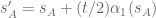 and
and 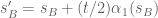 ) [Corrected, thanks – T.]
Also, while RH verification is a major project on its own, I was discussing with Rudolph earlier in the day that the barrier method, by creating a link between the verified height of zeta zeroes and the dbn bound would allow such a future project to lower the bound further (and also hopefully tighten the density estimates of the off-critical line zeta zeroes which would be a major motivation to do it, but the latter has been asked earlier by other commenters in different forms and probably is quite difficult to formalize).
I had referred to the 10^12 number due to Gourdon et al (although it’s not clear whether the large heights in their work were independently verified).
31 March, 2018 at 10:20 am
Terence Tao
Gourdon-Demichel claim to have verified RH for the first zeroes. Using the Riemann-von Mangoldt formula
  this suggests that
  can get up to about
  if one accepts the Gourdon-Demichel numerics. In any case I see your point that it can be worthwhile to obtain some results that is conditional on a numerical RH verification that could be feasible in the future even if it is not currently available. (e.g. “We can prove
  , but can improve this to
  if the first
  zeroes of zeta obey RH”, etc..).
31 March, 2018 at 5:15 pm
Anonymous
In “On running the mesh for each t step with c=0.05” what does c=0.05 mean? What is c and why is it 0.05?
31 March, 2018 at 9:08 pm
KM
At each time step, the rectangle (X,X+1,y0,1) is traversed using an adaptive mesh, and the c parameter is used to to ensure f=|a+b| does not go below c between the mesh points (the 0.05 value is arbitrary, but c should not exceed the expected min |f(z)|, otherwise the mesh will get stuck at a certain point) Now there is also a lower bound of |f(z_(i+1)|/2 if we choose c=0, so having a non-zero value may not be necessary.
1 April, 2018 at 9:07 pm
KM
One of the numerics participants had asked yesterday whether the t derivative bound estimated using the triangle inequality at the lower coordinates (X,y0,t0) has monotonicity properties for X,y,t and is good enough to act as a substitute for D, while jumping to t1 = t0 + c’/D. Here we are using c’ as (c + min|a+b|_t0_mesh)/2

From observations it seems that the bound decreases as t and y increase, and if we approximate the terms, we get a toy model like formula
whose values stay close (but not at the level of decimal points) to the exact bound. It does indicate the desired properties for atleast t and y. So we wanted to confirm that the bound calculated earlier is usable for the mesh calculations.
Also, we started with X=5*10^9+(0,1), y=(0.4,1), t=(0,0.2), moving forward in time t, and while it is somewhat slow, it is looking doable, and the computations get faster with time.
1 April, 2018 at 9:36 pm
Terence Tao
It might be possible to rigorously prove that the derivative bound is indeed monotone, but even if this isn’t easily done, I think it is close enough to being provably monotone that it will probably be safe to use the derivative bound at the lower values of , plus some safety margin, as the derivative for higher values of
  (keeping
  fixed of course). The main difficulty compared with the toy model is understanding the behaviour of the quantity
  , however the derivative of
  is quite small (of the order of
  ) and so one should be able to approximate its behaviour by a constant (e.g. by the value of
  at the lower values of
  ) with only a small error incurred. Once
  is replaced by a constant, it looks like one will get the desired monotonicity properties.
If one is able to evaluate for
for  comparable to the limits of numerical RH verification then there is probably no need right now to develop the potential third approach (based on trying to control sums like
  ) since at best this approach will also be limited by the same requirement to have numerics for RH.
6 April, 2018 at 12:51 am
KM
We ran the mesh for X=5*10^9 (N=19947), y0=0.4, t=0.2 and the winding number came out to be zero for each rectangle. The ddt bound used was the same as derived earlier. p15 or Anonymous likely completed it a few days back with a much faster script, and has also shared the script in another comment.
The winding number summary for the different t values is here and the detailed output of all the rectangles is here.
The large x formula in the wiki gives an estimate ~0.0555 at N=300000, y=0.4, t=0.2. Should we run the Euler mollifier bound between N=19947 and 300k?
Also, can we use a mollifier to lower the ddt bound (which would then provide a safety margin in this case)? I tried

and new_ddt_bound = mollified_ddt_bound/|mollifier|
which seems to result in a lower ddt bound for any x,y,t in the strip we have considered.
6 April, 2018 at 6:41 am
Terence Tao
Thanks for this! I’ve added these announcements to the zero free regions page on the wiki. I assume for the winding number calculations that the upper range of is
is  ?
?
If the Euler mollifier bound is feasible in the indicated range then it is certainly worth running, though this is about four orders of magnitude larger a range of x values which is a bit worrisome (but one should presumably be able to get some cutdown by improving the large x calculations, e.g. by using mollifiers; I did not seriously try to optimise those calculations as they seemed to be more than adequate back in the t=0.4, y=0.4 test problem). If it isn’t, one can raise y a little bit in this range at the expense of slightly worsening the bound on : the barrier you just constructed at
  automatically works for any larger value of
  without any further computation. (One also gets to lower t for free here, but this of course will make the large x calculations harder.)
6 April, 2018 at 8:03 am
KM
We had used the upper range of y as 1, although Rudolph had midway suggested based on the old result that y_max=sqrt(1-2t)+small epsilon could also be used, which we can do for future computations.
Also just wanted to mention that the mesh calculations were difficult and everyone contributed to optimizing and completing them.
6 April, 2018 at 9:17 am
Terence Tao
OK, thanks! If you have a list of contributors I can update the attributions on the zero free regions page accordingly (or if one of you has an account on the wiki you can do it directly).
To get a crude idea of how far one may be able to push the large x analysis, let us return to the toy model approximation and consider the question of when this is provably nonzero. The triangle inequality lower bound for this quantity is
so one has a chance of doing something as long as
It looks to me like this is actually the case at with quite a bit of room to spare (I get 1.076122 for the LHS), so one should be able to analytically verify this for larger N too (I had some tools for doing this at http://michaelnielsen.org/polymath1/index.php?title=Estimating_a_sum , basically evaluate a bounded number of terms numerically and then estimate the tail analytically).
For (in the regime
  , which is the case here) the corresponding triangle lower bound is
where and
and  is a moderately complicated quantity defined in equation (1) of http://michaelnielsen.org/polymath1/index.php?title=Controlling_A%2BB/B_0#Large_.5Bmath.5Dx.5B.2Fmath.5D_case but it looks like things are also good here (
 should decay like
  ). I haven't computed the E_1, E_2, E_3 errors but with N so large I would expect them to be quite small. So I think we may soon be able to clear all of the region
  , which would give
  without any further mesh evaluations! I might have some time this afternoon to write this out properly, hopefully in a form in which it will be clear how to adjust all the numerical parameters if needed.
p.s. regarding lowering y_max to , this will probably only be a modest saving since the main difficulty arises at t near 0, and also the derivative analysis gets a bit more complicated if the contour varies in time. It turns out that for related reasons one can narrow the thickness
  of the barrier a little bit to
  and even
  but again this would be a rather modest savings and perhaps not really worth the additional conceptual and coding complexity.
6 April, 2018 at 8:55 pm
Terence Tao
Oops, I made a numerically significant typo: the factor of should be
  , and the sum is now a lot worse at the t=0.2 level, the LHS that needs to be less than 2 is now 3.135 or so at N = 19947. (I guess I should have been more suspicious that the sum was so small!) So we are not close to knocking out the entire
  region just from the triangle inequality (even in the case of the toy approximation); it looks like N has to be something like 10 times larger, roughly matching what you had previously worked out. One may be able to get a bit further (as before) using Euler mollifiers and also the Dirichlet series lemma, but it does look like there will have to be a region that is covered by a numerical mesh.
6 April, 2018 at 7:31 pm
KM
Is the t factor in the denominator actually t/4. With that, the estimate increases to 3.129.
Also, the wiki seems to have a login but not a create account facility. Rudolph and David are the other two contributors.
Additionally, Anonymous’s script is likely fast enough that it’s possible to run the mesh (t=0.2,y=0.3,appropriate X) in reasonable time.
7 April, 2018 at 1:57 pm
Terence Tao
Thanks for pointing this out (I independently figured this out it seems, judging by the near-simultaneous comments).
Michael Nielsen locked down account creation on the wiki because of spam issues. You can contact him at mn@michaelnielsen.org to request an account. In any event I have added the attributions.
One thing that may be relatively quick to execute is to create a table of the minimal N, for given values of t,y, for which the toy criterion
holds (assuming for now that the sum is decreasing in N, as it appears to be numerically). One can then invert this table to find, for a given value of N, what the optimal value of would be, which would indicate roughly what we could expect to reach as a bound for
  for say
  without any further work. Then we could run the same exercise with some Euler mollifiers and see if there is significant improvement.
7 April, 2018 at 5:00 pm
Anonymous
For t=0.29 and y=0.29 I get t + (1/2)*y^2 = 0.33205 < 1/3 and the sum for the toy criterion with N=19947 is 1.99378 < 2. This is the best in a grid search with step size 0.01. The t and y were not constrained to be equal, it just turned out that way if I didn't make a mistake.
7 April, 2018 at 7:12 pm
Terence Tao
Thanks for this! The fact that should not be an issue, it contributes an additional error term in a number of estimates which will be very small for
  as large as
  (the additional error is roughly of size
  ). It’s likely all the remaining error terms (which are all of size
  or better) can fit inside the gap between 1.99378 and 2.
On the other hand, the barrier computations may become significantly harder with y reduced from 0.4 to 0.29, so it's not completely clear that we could get all the way down to 0.33205 this way. But it should be relatively easy to continue the barrier at up to time
  (the barrier calculations get faster as t moves away from zero) so we should have
  fairly cheaply this way, at least.
Given that we have some additional techniques (Euler mollifiers, mesh evaluations of A+B) to clear the region to the right of the barrier, probably the bottleneck is now how low one can lower the value of y in the barrier calculations. (One could also increase X a bit, since we're not quite at the threshold of the best RH verification in the literature, but I believe this would only lead to relatively modest gains and probably also make the barrier computations harder.)
7 April, 2018 at 6:08 pm
Anonymous
Some of the bounds need y >= 1/3, and y=0.29 is not in that regime.
8 April, 2018 at 3:11 am
KM
The Euler 3 mollifier with triangle inequality is positive (0.044) at N=19900,y=0.4,t=0.2
Similarly, the Euler 2 mollifier with triangle inequality is positive (0.056) at N=40000,y=0.4,t=0.2
If as in the Estimating a sum wiki, we fix N0=40000, that leaves the corresponding buffer for the tail sum (estimated from D*N0 +1 to D*N). Estimating the B and A parts of the tail sum numerically for different N values using a bisection method, it seems the B tail is less than 0.019 and the A tail (including the N^y denominator) is less than 0.017. There is a tradeoff as the summands decrease with increasing N, but the number of terms in the sum increase. The maximum is reached differently for the B and A tails near N=150k.
Is it possible to use two integrals here to bound the tail analytically? The alternate summand sequences seem to be decreasing, with the odd sequence similar to earlier. The even summand is a product of an increasing and decreasing term, hence it’s not clear how to prove its trend.
8 April, 2018 at 7:32 am
Terence Tao
The Euler 3 data is very promising, it brings us very close to getting when combined with the barrier. How fast is it to compute the Euler 3 bound for a given value of N? If we can use it to clear, say, the region
  , then we only need to do analysis past
  , and here the ordinary triangle inequality bound seems to work, thus avoiding the need to work out what the Euler 3 tails look like. One could also imagine splitting the range
  and using Euler 3 for the lower part (e.g.
  ) and the (presumably faster) Euler 2 bound for the upper part.
8 April, 2018 at 5:45 am
KM
I tried to derive formulas for some parts of the Euler 2 mollifier based tail using the wiki approach, assuming N>2N_0.
The even terms with n < N look more difficult.
8 April, 2018 at 11:00 am
KM
The E3 mollifier currently takes 6 to 12 seconds for each N (20k to 40k), while the E2 mollifier takes around 2 to 10 seconds (40k to 2*10^5).
At 2*10^6, the E2 mollifier takes around a couple of minutes.
It should be possible to makes this 2-3X faster through some simple means, and probably it can go much faster if done in a faster library.
Also wanted to confirm on the 2*10^6 part, since the non-mollified bound including the tail seems to turn positive in the lower 10^5 magnitude (with N_0 of a similar magnitude).
8 April, 2018 at 12:41 pm
Terence Tao
Sorry, that was a typo, I meant . So it looks like we can use E2 and E3 to cover the
  region in a somewhat reasonable amount of time (less than a month, presumably less with some speedup). One potential way to speed things up is to do something like a mesh, e.g. only compute the bounds for N a multiple of 10, and get some upper bound on how the bound changes when one moves from N to N+1 (basically, differentiate each summand in N, add up bounds for each that are uniform in the interval [N,N+1], and add the additional N+1^th term). In any event even a crude mesh (e.g. spacings of 100) should give the right picture as to how much room there is to insert all the error terms (but I expect that with N this large, all the error terms are going to be well below dangerous levels).
9 April, 2018 at 11:25 am
KM
Thanks. We will start working on this.
Also, few days back I had tried deriving an N dependent ddt bound as a replacement for the x dependent one. The derivation is kept here. After checking it for many different values of N,y,t (with N large), it seems to be around 1.2X of the x dependent bound, and we kind of hit a wall. Does the derivation seem correct and is it possible to improve the bound further using this approach?
9 April, 2018 at 7:11 pm
Terence Tao
The denominator lower bounds aren’t quite right, you need to lower bound , and this is not necessarily bounded from below by
  , though the value of
  comes quite close to being a lower bound here. For
  , you can do slightly better by using Pythagoras theorem
  rather than the triangle inequality bound
  , getting something like
  .
.
10 April, 2018 at 8:02 am
KM
Thanks. I think in the denominator I had used as a proxy for
  Is the issue with
  that
that  can be negative and should be accounted for? I tried estimating a lower bound for this term as well.
10 April, 2018 at 8:25 am
Terence Tao
Yes, this was the issue, though the effect of this term on the derivative bounds should be very small, especially in the most dangerous region when t is close to 0.
29 March, 2018 at 3:49 am
Nazgand
It just occurred to me that counting the zeroes on the real line may be easier. Zeroes don’t just suddenly appear or disappear, so track a zero, r, at the edge of the boundary, then count the number of zeroes on the real line between z=0 and z=r’. If the number of zeroes is the same, the de Bruijn-Newman can be lowered.
If this plan would not work, I would like to know why. Calculating along the real line rather than a rectangular chunk of the complex plane just seems easier.
29 March, 2018 at 7:16 am
Terence Tao
Unfortunately, the potential problem is that even if the real zeroes are completely frozen in time, one or more pairs of complex zeroes could fly in at high speed from horizontal infinity, passing above a large number of the real zeroes, potentially leading to a zero for a large value of
  (e.g. t = 0.4) with a large value of y (e.g. y=0.4), while still being consistent with the ability to preclude such zeroes for large values of x.
A key difference here between the real and complex numbers is that the real numbers are totally ordered, so that zeroes cannot move past each other without colliding, whereas complex numbers are unordered, and zeroes can move past each other in complicated ways.
29 March, 2018 at 3:17 pm
David Bernier (@doubledeckerpot)
Can checking the absence of zeroes of for
for  be reduced to checking for only finitely many values of
  ?
?
29 March, 2018 at 4:32 am
Anonymous
It would be nice to include in the main page (as done e.g. in polymath8) an updates table of upper bounds records.
29 March, 2018 at 7:21 am
Terence Tao
I think what might work is to have a table of known zero-free regions for the equation , e.g.
  , and keep a separate column for the optimal value of
  that can be deduced from all of these zero-free regions. I might work on such a table later today.
29 March, 2018 at 9:44 am
Terence Tao
The table is now in place at http://michaelnielsen.org/polymath1/index.php?title=Zero-free_regions . Hopefully I have the attributions and dates correct. Any corrections welcome (Actually everyone is welcome to create an account on the wiki to edit the wiki directly also.)
30 March, 2018 at 5:08 am
Anonymous
It is still not sufficiently clear from this table how the sides of the whole rectangle ( and
and  ) where tested by the argument principle to show it to be
  zero-free for
  (in particular, it seems that the horizontal interval
  for
for  is missing from the table, as well as the right vertical side with
  of the whole rectangle.)
30 March, 2018 at 7:14 am
Terence Tao
For the region we don’t need the argument principle and can establish non-vanishing of
  directly as follows. Here what one does is obtain lower bounds on
  and upper bounds on the error
  . The former had already been lower bounded for
  using Euler product mollifiers and variants of the triangle inequality in the
  case, but one nice feature of these arguments is that the bounds always improve as
  increases, so the lower bounds extend automatically to
  . Now, on the other hand, the upper bounds on the error degrade slightly as
  increases (in particular there is an annoying
  factor in the main error term
  , see e.g. Proposition 5.3 of the writeup), but I think there is enough room (particularly with recent slight improvements to this error term) to accommodate this loss.
30 March, 2018 at 10:51 am
KM
Despite the 3^y factor, the error bounds seem to decrease as y increases. The [T’/(2*Pi)]^[-(1/4)*(1+y)] factor exerts more influence even at low values of N. For example, |h-(a+b)| error bound for some (N,y) pairs:
N, with y=0.4, with y=0.45
3, 0.932, 0.917
10, 0.154, 0.147
50, 0.0148, 0.0135
Also, with t=0.4, y=0.3, the euler5 mollifier with the lemma bound (as in the wiki, maybe slightly different from the paper) gives a positive lower bound for |a+b| at N=319 (compared to N=192 with t=0.4, y=0.4). Earlier we had run the mesh upto N=300, but since the error bound is quite low by this point, and even a slight increase in N helps |a+b| stay above it, is it fine to run the mesh for y=0.3 upto N=350?
30 March, 2018 at 12:17 pm
Terence Tao
Ah, good point! The error term degrades relative to
  as
as  increases, but improves relative to
  due to the
  factor. Conversely, it means that it will cause more trouble as we lower y.
Certainly there’s nothing particularly special about 300, if it looks like mesh evaluations of can be stretched up to 350 for instance then we can shift the transition point to using Euler product mollifiers etc. to later. I think that the low x calculations should be fairly insensitive (as far as run time and accuracy go) with the values of
  and
and  , so hopefully we should always be able to cover the region
  (or
(or  ) numerically. (There are some factors of
  in some of the derivative bounds, but as long as we don’t send t to be very small, I don’t think this will hurt us that much, e.g. one should still be OK for say t=0.2, and I doubt we want to go much below that in any case unless we are trying the second approach (based on barriers) to getting zero free regions.)
29 March, 2018 at 5:00 am
Anonymous
It seems somewhat easier to start with lowering below
below  while keeping
  . A good start seems to be
  (which should give
  )
)
29 March, 2018 at 9:50 am
Terence Tao
One minor observation is that by keeping fixed, one can reuse some of the previous calculations, for instance the
  data can be reused without any modification.
31 March, 2018 at 2:28 am
rudolph01
Using the 3rd approach integral, a clockwise run around the rectangle for
for  confirms and stretches Anonymous’ earlier result that
  does not vanish in this region. It ran for roughly 8 hours. Please find the output below.
Run x=0..3000 y=0.4..045 t=0.4
[Added to wiki, thanks! – T]
29 March, 2018 at 7:49 am
Anonymous
Dear Prof. Tao, I am not sure if there is a typo in the last inequality about S(t).
http://michaelnielsen.org/polymath1/index.php?title=Dynamics_of_zeros
According to Groenwall’s inequality, the function S(t) should be bounded by S(0), while in the wiki page it is bounded by S(t) itself.
[Corrected, thanks – T.]
30 March, 2018 at 7:22 am
Terence Tao
One relatively easy numerical exploration that we can do is to get some sense of the ranges of for which the quantity
  stays reasonably close to 1 (enough so that we have a chance of verifying that it does not wind around the origin). In the
  case it seems that this happens all the way down to quite low values of
  (e.g.
(e.g.  , or
, or  ), and we had already seen that increasing
  tightens the clustering (see e.g., this plot of KM’s, with the orange dots being the
  values of
  and the green dots being the
  ). Conversely, as we lower t and y (or go to smaller values of x) we will get more of a spread and eventually we will lose control of the winding number. Perhaps for various values of (t,y) we could numerically locate ranges of x (or of N) for which a coarse mesh evaluation
  behaves well enough that we have a hope of working out the winding number? (One of course also has to deal with the error terms, but the bounds we have on these terms do not get much worse as we decrease t,y, in fact they might actually improve slightly in some cases.)
30 March, 2018 at 7:53 am
Anonymous
It seems that the analytic threshold (which is related to the analytic threshold
  ) should be quite sensitive to changes in
  (in particular for small
  ).
).
31 March, 2018 at 6:51 am
Anonymous
Does http://michaelnielsen.org/polymath1/index.php?title=Bounding_the_derivative_of_H_t_-_third_approach provide bounds of the derivative of Ht that apply to intervals of x? There might be blog comments or github comments about how it’s trivial to do with the triangle inequality, but it would be helpful to me to see it on the wiki.
31 March, 2018 at 3:47 pm
Terence Tao
The dependence of bounds on and
and  on
on  as given in the wiki is quite simple, so one can just use monotonicity. For instance, if
  ranges in the interval
 ![[x_1,x_2]](https://s0.wp.com/latex.php?latex=%5Bx_1%2Cx_2%5D&bg=ffffff&fg=545454&s=0&c=20201002) , then
, then  will not exceed
  , so one can use that to upper bound
  to obtain bounds for
  that are uniform in that interval.
31 March, 2018 at 7:25 am
Anonymous
Suppose that (with some fixed (large)
  ) for any
  (with some fixed
  ) and any
  . Is this “zero width barrier” sufficient to show that if
  is zero-free in the region
  so is
so is  for any
  ?
?
31 March, 2018 at 8:19 am
Terence Tao
I don’t know how to achieve this, because i need a thick barrier to prevent a zero sneaking under the barrier and then being pulled upwards by the attractive force of a higher up zero to the right of the barrier. This is a very implausible scenario, but not one I know how to rule out with a zero thickness barrier. On the other hand, by the argument principle, verifying that a two-dimensional region is zero-free is actually not that much harder than verifying a one-dimensional region.
1 April, 2018 at 11:48 am
David Bernier (@doubledeckerpot)
If we wanted a name for the functions , one possibility would be to refer to these as the “de Bruijn-Newman family of functions
  “, or the “de Bruijn-Newman functions
  .
.
1 April, 2018 at 12:36 pm
Anonymous
Does this function already have some combination of names, identifiers, symbols, characters, data, or conductors or whatever in http://www.lmfdb.org/?
1 April, 2018 at 12:59 pm
David Bernier (@doubledeckerpot)
I doubt these parameterized functions are “real” L-functions. Unless I’m mistaken, should have non-real zeroes.
 designation, please see his comment here https://terrytao.wordpress.com/2018/03/18/polymath15-sixth-thread-the-test-problem-and-beyond/#comment-494089 .
Prof. Tao searched the literature for the origin of the
Perhaps Csordas, Varga et al deserve some credit too.
1 April, 2018 at 1:24 pm
Anonymous
Let’s use the distinguished naming procedure that led to coining “tropical geometry.” Begin by a identifying a person prominently associated with the concept. For tropical geometry it was Imre Simon. In our case we have Nicolaas Govert de Bruijn. Next, identify where that person is from or where they live. For Imre Simon it was Brazil and for de Bruijn it was the Netherlands. Finally, identify a stereotypical or even vaguely racist property of that location or nationality. For Brazil it was “tropical”. For the Netherlands I’m not sure what to use. The Dutch are stereotypically tall and wear clogs and ride bicycles, so let’s call it the “tall H function”.
1 April, 2018 at 1:48 pm
Anonymous
“clogarithmic H function”
“bicyclic H function”
1 April, 2018 at 5:17 pm
David Bernier (@doubledeckerpot)
I was thinking that going into negative region, one should soon see Lehmer pairs and almost-Lehmer pairs of zeroes collide and move away from the real line, following the evolution of the zeroes of the
  with
with  decreasing from zero…
2 April, 2018 at 7:30 am
Terence Tao
Yes, it is now known that for any negative t, there must be non-real zeroes. Presumably one could see this numerically (I vaguely recall someone doing this a few weeks ago). The methods to compute in http://michaelnielsen.org/polymath1/index.php?title=Bounding_the_derivative_of_H_t_-_second_approach should continue to work without much modification for negative
  (indeed the convergence should be even better now). The methods in http://michaelnielsen.org/polymath1/index.php?title=Bounding_the_derivative_of_H_t_-_third_approach are more problematic, but the first equation on that page should still give a correct and convergent formula (bearing in mind that
  is now imaginary – it doesn’t matter which branch one takes), even if the remaining contour integration and tail bound estimates are no longer valid as stated. Also I think the
  and
and  approximations should still be reasonably accurate, though the rigorous error bounds currently in the wiki or pdf writeup no longer apply. If someone has spare time and numerical capability on their hands they are welcome to experiment with the
  regime; as far as I can tell it won't directly impact the primary goal of this project, but may help deepen our general intuition regarding the behavior of the
  (and on the reliability of various numerical approximations).
4 April, 2018 at 1:43 pm
rudolph01
Using the first equation from the third integral approach, and verifying the data with , here are some implicit plots for the
  domain.
The first picture shows some complex zeros for in the x,t-plane, fortunately all below
  :), and the plot also illustrates the intriguing complexity in this domain.
In the second picture,the trajectory of a single complex zero is followed all the way till its unavoidable collision with its conjugate.
Few initial observations/questions: , all complex zeros that I tested appear to also march up leftwards (and of course also towards their conjugates). Is this true/provable?
 , appear to have to ‘surround’ multiple complex zeros at less negative
  (see second picture). Does this imply that the density of complex zeros has to decrease when
  goes increasingly negative?
* Similar to the real zeros, above a certain
* Complex zeros that reside at a more negative
4 April, 2018 at 3:22 pm
Terence Tao
Thanks for these graphics! I think all zeroes should in general experience a leftward “pressure”, coming from the contributions to the velocity
  coming from those zeroes
  at distance to
  comparable to
  . At most scales, the zeroes to the right and to the left of
  should exert a roughly equal “force” on the
  zero that more or less cancels out, but at the scale
  , there are more zeroes on the right than on the left (because zeroes are sparser near the origin than away from the origin), and so all zeroes (real or complex) should move leftwards on the average. But occasionally they can be influenced by more short-range interactions to go against this trend.
I’m not sure I understand what you mean by complex zeroes “surrounding” other complex zeroes, though. One would expect to have more and more complex zeros as t becomes more negative, as the remaining real zeroes collide and become complex; though at some point this process exhausts all the real zeroes and then the number of complex zeroes in a given region should stabilise (other than marching to the right on average as t increases, as discussed earlier).
4 April, 2018 at 7:52 pm
Anonymous
It seems that (similar to the “attraction” of complex zeros to the real axis – due to their vertical attraction to their complex conjugates) their is a similar horizontal “repulsion” of complex zeros from the imaginary axis – due to their horizontal repulsion from their images with respect to the imaginary axis. In this sense, the imaginary axis is acting like a barrier for complex zeros in the right-half-plane moving leftward.
In particular, it seems that the imaginary axis, acting as a “barrier”, should be zero-free for any real t.
4 April, 2018 at 9:03 pm
Anonymous
In fact, for any real
  , since the integrand in its defining integral is clearly positive in this case.
5 April, 2018 at 8:23 am
Terence Tao
That’s a nice observation – simple, but somehow I missed it before. I was initially a bit confused because this graphic indicates that is negative real rather than positive real on the imaginary axis, but this is because
  is negative there.
Anyway, now we understand the left side of the region very well. Not that this was the most dangerous side in any case, but every little bit helps…
2 April, 2018 at 9:13 am
Anonymous
I did ask a question about the evolution of a Lehmer pair when t varies, and the Polymath 15 participant Rudolph generated several beautiful graphs here:
3 April, 2018 at 12:07 am
Anonymous
If , we know that
  has finitely many (
 , say) non-real zeros for each
  . Hence, by fixing
  , we see that
  is a positive, bounded, non-increasing, integer-valued function on
  with
with  – meaning that by letting
  , the last non-real zero of
  (with its complex conjugate) should arrive to the real axis precisely for
  – showing that
  must have a multiple (real) zero (assuming
  .)
.) (i.e. RH !) is implied by requiring
  to have only simple zeros.
The conclusion is that
4 April, 2018 at 11:34 am
Anonymous
In the wiki page on the dynamics of zeros, the limit expressing the zero velocity should apply to the expression inside parentheses.
[Corrected, thanks – T.]
5 April, 2018 at 4:38 am
rudolph01
Just for fun, I have prepared two visuals that attempt to explain our latest approach to keep complex zeros out of the ‘forbidden’ zone < X. Hope they are a reflection of what's really going on, but at least these already helped me a lot to explain the De Bruijn-Newman constant to my family :)
5 April, 2018 at 8:35 am
Terence Tao
These are indeed nice visuals – it is hard to depict what is going on in the directions simultaneously, but it does seem possible to do so with your visuals (though I had to think a little bit to convert it back to my own mental imagery, where
  is a time variable rather than a spatial one, so that one thinks of 2D videos of zeroes flying around, rather than 3D worldlines of zeros).
5 April, 2018 at 8:54 pm
Anonymous
Here’s a C/arb script for the winding number for f(z) = (Aeff(z) + Beff(z))/Beff0(z).
https://pastebin.com/5ngVh4QG
At its core is a procedure that uses forward mode automatic differentiation and interval arithmetic to obtain uniform bounds on |f’| on segments of the contour. These segments are recursively split, the bounds are refined, and f is evaluated at segment endpoints until |f| is proven to be greater than c on all segments.
The usage notes follow…
—
Usage:
./a.out N c t xa xb ya yb
This script computes the winding number about 0 of f(p).
Let r be a rectangle in the complex plane
r : [xa <= x <= xb] + i[ya <= y <= yb]
and let p be the counterclockwise path along the boundary of r
starting and ending at (xa + i*ya).
Let f(z) = (Aeff_t(z) + Beff_t(z)) / Beff0_t(z).
Additionally, f(p) is required to stay away from 0 so
the script will either abort or will fail to terminate
if |f(z)| <= c at any point z on the path p.
The Nth partial sum is used in Aeff and Beff.
9 April, 2018 at 6:05 am
Anonymous
Is it possible to show (for suitable ) that
  by showing that
  has only real zeros?
A natural strategy consists of
1. Showing analytically that has only real zeros if their real parts are above a sufficiently good explicit numerical threshold
  .
.
2. Showing that there are no non-real zeros in the rectangle
  by counting the number of zeros inside this rectangle (using the argument principle) and comparing it to the number of real zeros in this rectangle (counting sign changes – using sufficiently good approximations of
  (obtained e.g. by tracking the time dynamics of
  zeros – starting with approximate zeros of
  as computed e.g. in Platt’s paper.)
9 April, 2018 at 8:55 am
Terence Tao
This would basically be the limiting version of our current strategy when is set to 0 rather than something like
  . While this does have the advantage of allowing one to increase
  (since currently we are using the bound
  ), there are some non-trivial difficulties in executing your steps 1 and 2 in the y=0 setting. For
  away from zero, there is an imbalance between the two main terms
  in the approximation for
  that makes it relatively easy to establish a zero-free region. It is possible to asymptotically push this down to
  using some additional tricks based on the argument principle and Jensen’s inequality, as is done in the current writeup but it involves a number of unspecified constants and would probably lead to a numerically large value of
  .
.
Evolving the time dynamics of zeroes is going to be computationally quite difficult – this is a system of ODE involving an infinite number of zeroes, all but a finite number of which we don’t actually know the value of! In principle there is this potential scenario in which a whole bunch of non-real zeroes of , lurking just outside the numerical verification of RH, zoom in at high speeds to small values of
  , and then mess around with the locations of the numerically visible real zeroes and move them to strange locations. For large values of
  we can erect a barrier to stop this scenario from happening, but it looks significantly harder to do so near the real axis.
9 April, 2018 at 9:56 am
Anonymous
I meant to evolve the time dynamics not via the (numerically problematic) infinite ODE system, but by following the dynamics of each zero from
  to
to  with sufficiently small “time steps” such that the k-th zero
  of
of  should converge (by fast local root finding algorithm) to the corresponding zero
  of
of  .
.
If the number of zeros in the rectangle (computed by the argument principle) would be equal to the number of real zeros in the rectangle (computed by sign changes) then it should imply that all the zeros in this rectangle are real.
9 April, 2018 at 6:35 pm
Terence Tao
I just added to the writeup a proper treatment of the very large x case when and
and  , namely when
  , using the triangle inequality and bounding all error terms and tails. I had previously thought
  would suffice for the triangle inequality bound, but it seems fall just a little bit short, even if one uses the lemma to sharpen the bound slightly. This may make things a little more computationally challenging for the Euler2 portion of the verification, but hopefully we can get a mesh argument to work.
10 April, 2018 at 3:59 am
Anonymous
In the writeup, in the line below (11), it seems that “zero” should be “nonzero at the origin” (as in the wiki sub-page on zeros dynamics.)
10 April, 2018 at 6:04 pm
KM
The Euler2 mollifier bound data for t=0.2,y=0.4,N 40k to 100k with stepsize of 100 is kept here. The bound reaches 0.2 around N=60k and 0.3 around N=85K. The change between successive values (N+100,N) also seems to be gradually decreasing.
10 April, 2018 at 7:48 pm
Terence Tao
I’m a bit confused as to what the bound represents; I would have expected the lower bound for to be decreasing with
  , not increasing as this table seems to suggest. Could you clarify what euler2_moll_bound is measuring?
10 April, 2018 at 9:36 pm
KM
I calculated where b_n and a_n are the mollified terms and a_n includes (n/N)^y, exp(delta) and other terms. Also, from the t=y=0.4 exercise, the function turns positive at N=478.
11 April, 2018 at 6:30 am
Terence Tao
Ah, ok, thanks. Actually the bound should be decreasing in N; I don’t know why I thought it would be increasing.
I’ll try to see if there is some reasonable way to control the size of the difference between the bound at N and the bound at N+1. If one can get it under 0.002 or so then the step size 100 mesh should be fine; otherwise we have ot increase the mesh size a bit (or try to also control second differences or double derivatives, but this looks a bit messy).
11 April, 2018 at 9:21 am
KM
These are some ddN values I got for the Euler2 toy bound (using the 2 – Sum_B – Sum_A formula). Values were verified against the newton quotient. They do seem to be well under 0.002 (excluding the additional terms at N+1, which seem to be smaller than the derivative).
t=0.2,y=0.4
N, ddN
40k, 1.32*10^-5
100k, 3.25*10^-6
200K, 1.10*10^-6
11 April, 2018 at 11:35 am
KM
Also, since all the multipliers and summands in the calculated ddN formula are positive, is it fine to estimate the lower bound of |a+b| for intermediate N points as lower_mesh_point_estimate – additional terms. Or do we have to penalize the mesh estimate with something like -ddN*1?
11 April, 2018 at 11:51 am
Terence Tao
Yes, if we let be the lower bound for
  , extending the definition to non-integer
  (with jump discontinuities at each integer), and if we have a derivative bound of the form
  for all non-integer
  in an interval
 ![[N_0, N_0 + M]](https://s0.wp.com/latex.php?latex=%5BN_0%2C+N_0+%2B+M%5D&bg=ffffff&fg=545454&s=0&c=20201002) and a jump discontinuity bound of
and a jump discontinuity bound of  at each integer
  in that interval, then we have
  throughout
 ![[N_0,N_0+M]](https://s0.wp.com/latex.php?latex=%5BN_0%2CN_0%2BM%5D&bg=ffffff&fg=545454&s=0&c=20201002) . Actually we can do a bit better than this by also working backwards from
. Actually we can do a bit better than this by also working backwards from  , but given how good the bounds on
  are (and I am guessing
  will also be very good, it should be about
  the size of the whole sum given that it comes from just a single term) we probably don’t need to be too sophisticated (it would only save a factor of two at best anyway).
11 April, 2018 at 1:14 pm
KM
In the E2 mollified sum, it seems there are 3 terms (in B and A each) which change or get added as N increases by 1. The two terms n=2N+1 and 2N+2, although the first one is zero, and also the n=N+1 term due to the delta function. Should we consider the 2M non zero terms while deriving MJ? I also tried deriving a bound for MJ (dropping any conditional negative part from the first M affected terms).
Also, should we set M as stepsize-1?
12 April, 2018 at 10:59 am
KM
The previous proposed formula for MJ had some typos regarding mods. Also, by removing any subtractions and making the formula simpler and conservative, is it fine to take MJ (including the A sum contribution) as
For t=0.2,y=0.4,N=40K,M=99, the above estimate comes out to ~ 0.00056.
11 April, 2018 at 11:07 pm
Anonymous
Here’s a C/arb script to compute the Euler mollified dirichlet series lower bound of abs(Aeff + Beff)/abs(Beff0).
https://pastebin.com/WZi63kCq
Usage notes and examples follow…
—
Usage:
./a.out t y Na Nb Nstep m n d
This script computes a lower bound of abs(Aeff + Beff)/abs(Beff0)
for N between ‘Na’ and ‘Nb’ with steps of size ‘Nstep’.
It uses an Euler mollification that includes m primes,
so that for example m=0 corresponds to no mollification
and m=3 corresponds to an Euler mollification that uses
the first three primes {2, 3, 5}.
Each row of output consists of N followed by the bound
and n derivatives with respect to N, so that for example
n=2 would print rows consisting of N, the bound,
the first derivative of the bound with respect to N,
and the second derivative of the bound with respect to N.
All output has d significant decimal digits of accuracy.
—
Examples:
./a.out 0.4 0.4 321 322 1 2 1 10
321 -0.0003790530744 0.002782680281
322 0.001790379319 0.002767556381
./a.out 0.4 0.4 477 478 1 1 1 10
477 -0.001301082303 0.001626307626
478 5.427798648e-05 0.001620293615
./a.out 0.2 0.4 20000 20000 1 0 1 10
20000 -1.127467428 4.94147775e-05
./a.out 0.2 0.4 20000 20000 1 1 1 10
20000 -0.243596499 3.68902378e-05
./a.out 0.2 0.4 20000 20000 1 2 1 10
20000 0.04755850292 3.381699674e-05
./a.out 0.4 0.4 500 500 1 1 1 10
500 0.02370202975 0.001510382076
./a.out 0.4 0.4 500 500 1 2 1 10
500 0.2259563455 0.00138754766
./a.out 0.4 0.4 500 500 1 3 1 10
500 0.2935839092 0.001354301778
time ./a.out 0.2 0.4 40000 100000 100 1 1 10 | tail -n 3
99800 0.3411359593 3.256440052e-06
99900 0.341388428 3.251396669e-06
100000 0.3416405273 3.246366034e-06
real 3m43.574s
12 April, 2018 at 6:18 am
Anonymous
Here’s the output for the 384 minute run of
./a.out 0.2 0.4 40000 300000 10 1 1 10
https://gist.githubusercontent.com/p15-git-acc/5298cb724b7731641ae203abe5d6ed2a/raw/e442ce9e28b24e0a201abb5b462521e68d2a4e42/gistfile1.txt
12 April, 2018 at 10:02 pm
Anonymous
Here are the E2 mollified bounds for all N between 40000 and 300000 (step size 1). t=0.2 y=0.4.
https://gist.githubusercontent.com/p15-git-acc/17ef55b4143a6cc9e7c082004ca185f5/raw/b937bbb2b1d9e2a85fe457984ee993a75107595f/gistfile1.txt
Together with Rudolph’s E3 mollified bounds calculation (linked below) for all N between 19947 and 40000 (also step size 1 and t=0.2 y=0.4) this may help with the intermediate sizes of in a
in a  proof.
https://github.com/km-git-acc/dbn_upper_bound/files/1904955/Output19947to40000.txt
13 April, 2018 at 8:50 am
Terence Tao
Thanks for this! I have added it to the wiki.
It looks like we are now close to clearing the middle range . The path of least resistance may simply be to run your code with mesh size 1 rather than 10 so that we don’t have to do any derivative analysis; if the 10-mesh run took 384 minutes then the mesh 1 run should take three days (also it could be parallelised simply by chopping up the range into pieces; one could also save 10% of the work by reusing the existing mesh when N is a multiple of 10). But it looks like the derivative bound approach would work also (now that we have an extra order of magnitude of room coming from working with a mesh of 10 rather than 100).
If one combines that with an Euler3 calculation in the remaining range and E_1,E_2,E_3 estimates in
  then we seem to have filled in all the jigsaw pieces to prove
  . This may well be a good place to declare victory; one may be able to shave a 0.01 or so from this bound by pushing a little bit further, but I think we are already beginning to hit the limits of the method (and progress is roughly inversely logarithmic to the amount of computer power thrown at it, so that’s not really the bottleneck). I guess we could do some exploratory calculations though to see if there is any relatively cheap way to lower the t or y parameters further while keeping the lower bounds for A+B/B away from zero.
13 April, 2018 at 8:58 am
Anonymous
“The path of least resistance may simply be to run your code with mesh size 1 rather than 10 so that we don’t have to do any derivative analysis” The 384 minute run used mesh size 10, but the later one and Rudolph’s have already used mesh size 1!
13 April, 2018 at 8:50 am
Anonymous
I should clarify that by “E2 mollified bound” I meant the lower bound of |Aeff+Beff|/|Beff0| computed with the Euler product mollification of the dirichlet series, where the largest prime in the Euler product is 2. At least that’s what I think I mean. Same thing with Rudolph’s E3. I was using the E2 and E3 terminology because I saw other people using it, but now I see that it’s confusing with the error terms E1, E2, E3 and I should have said Euler2 and Euler3 instead.
13 April, 2018 at 8:57 am
Terence Tao
OK, thanks for the clarification! I’m correcting the wiki now to reflect this. I guess we can agree to use Euler1, Euler2, Euler3 for the mollified bounds and Error1, Error2, Error3 for the error bounds to avoid misunderstanding.
Also, on closer rereading I now see that you’ve already done the mesh 1 calculation for the mid range . So it looks like we don’t have to do any derivative analysis in N at all! So, it seems like the only remaining computational task is to compute Error1, Error2, Error3 in the
  ranges, which should be relatively quick compared to the other tasks already completed. (Note that the formulae on the writeup are slightly different from that in the wiki.)
13 April, 2018 at 1:25 pm
KM
Given the speed at which the current scripts output results, I was just checking the feasibility at t=0.2,y=0.3, and things seem quite feasible for a follow-on exercise later. Euler 3 triangle bound at N=69098 (x ~ 6*10^10) is ~ 0.22, and the non-mollified bound at N=600K is 0.0564.
At t=0.15 and y even at 0.4, N=10^7 gives a positive non mollified bound, but at N=69098 all the mollified bounds considered so far (Euler 2/3/5, with triangle/lemma are sufficiently negative).
14 April, 2018 at 8:00 am
Terence Tao
That’s more promising than I thought! But I would imagine the real bottleneck would be the barrier computation. Still I guess we could shoot for a nice clean bound this way…
14 April, 2018 at 5:45 am
KM
There seems to be a small typo on pg 21 of the paper for the errors e_C and e_C,0. The 6.72 factor should be 6.92 according to pg 24.
[Corrected, thanks – T.]
14 April, 2018 at 10:17 am
Anonymous
Some of the estimates and bounds currently require y >= 1/3. Would these need to be reworked for smaller y if we go for t=0.2 y=0.3?
14 April, 2018 at 10:49 am
Terence Tao
Some of the wiki estimates have this restriction, but the writeup estimates have been written so as not to need these. (Note in particular the factor of Proposition 6.6(ii), which activates once
  goes below 1/3.)
15 April, 2018 at 3:33 am
KM
The writeup doesn’t seem to have the ddx bound formula yet (present at the bottom of the Controlling A+B/B 0 wiki). In the wiki, it mentions the y>1/3 restriction for this bound. If we go below y=1/3, will this bound change as well?
Also, there seems to be a typo on pg 22 of the writeup, where the 2(1-y) factor while bounding Re(alpha(s)) should be -2(1-y). On checking against the final bound for Re(alpha) at some x+iy, for eg. x=1000,y=0.5, we seem to get a small negative difference for Re(alpha)-bound.
15 April, 2018 at 12:48 pm
Terence Tao
Thanks for pointing out the typo, which actually required a non-trivial rewrite here; the restriction needs to be replaced by the slightly more restrictive
  , though at y=0.4 this is still certainly safe. I’ll work on the writeup to fix this; also will put in some more details on how to deal with the medium ranges of N and to extend the derivative bound below this restriction (I guess this is needed to extend the barrier calculations below y=0.4).
15 April, 2018 at 12:24 pm
Rudolph01
We have started work on the remaining computational task to compute Error1, Error2, Error3 bounds in the range to complete the
  case. These error bounds are named eA, eB and eC0 (since we are not using
  ) in the write-up. Here are some sample data (respectively eA, eB, eC0):
5.2812559935137…e-11
7.2181152722662…e-10
7.2698636640998…e-6
8.3090086061558…e-13
2.8949570104373…e-11
4.1858191562622…e-7
1.3746978215374…e-13
7.3836305552204…e-12
1.1325230648234…e-7
4.8124550500060…e-14
3.3324044232747…e-12
5.1555261007475…e-8
All error bounds seems to be monotonically decreasing and the overall bound is dominated by eC0 with eA and eB a few orders of magnitude smaller. When eC0 was first derived on the wiki,wiki (The Estimating E3 section), it was proved to be monotonically decreasing. Is that still the case for latest version of eC0 in the write-up?
Now, if eA and eB are much smaller than eC0, and eC0 is monotonically decreasing with its delta at each successive N much larger than any possible increase in eA or eB, then are the error bounds required to be evaluated at each N or could we take steps of say ?
?
Here is the output of a test run (in steps of , accurate at
  digits) for
  .
.
15 April, 2018 at 1:49 pm
Terence Tao
Thanks for starting this! The bound for in Proposition 6.6(vi) is indeed monotone decreasing in
  once
once  is larger than say 200; this is clear from inspection except possibly for the term
  , but Lemma 5.1 ensures that
  is decreasing, and so is
  , so the claim follows from multiplying.
The bound for in Proposition 6.6(iv) is at most
  times the corresponding bound for
  . This factor
  can be bounded by
  which is only a little bit larger than 1, in particular it should be easily bounded by 2 in the range of interest. So up to a factor of say 3 we can ignore
  and just bound
  .
.
One can bound in a range such as
  by using the upper bound
  for the summation range of
  and the lower bound
  for the value of
  in summands, if we bound
  by
by  (here we use that $\frac{\log^2 \frac{x}{4\pi}}{\frac{x}{2}-3.33}$ is monotone decreasing for
  ), thus getting the somewhat crude bound
(and then using the lower bound for and again substituting
  for
for  ) but given your numerical data I would imagine that this bound will still be more than serviceable.
16 April, 2018 at 2:10 pm
Rudolph01
The new, “step” bound formula for provides a great speed boost :) Below are the outputs for respectively step sizes
  . The fields are:
  .
.
Further optimisation could be done by calculating only once at the start of the range, rather than for each
  .
.
I have used the most recently updated definition of from the write-up, but since we are using
  and a sufficiently large
  , there is no difference compared to the previous version.
Since all values of the upper bound of the error terms stay way below the lower bound of , does this complete our
  case?
case?
Step 1000
Step 10000
Step 100000
17 April, 2018 at 7:30 am
Terence Tao
Great! It does seem that we have indeed finished off the numerical verifications needed to show that . In this particular case the bounds for
  are so small that one can probably use some of the analytic techniques currently used in the
  case to safely cover this range also, but this sort of numerical verification could be useful if we want to make one last push to say
  (one could joke that this is “halfway towards RH :)”).
I’m in the process of putting the derivative bounds on A+B/B in the writeup, trying to clean things up a bit from the wiki version. Nearly done with the x and y derivative bound, will also work on the t derivative bound which is not currently on the wiki.
17 April, 2018 at 9:59 am
KM
We were able to test the (A+B)/B0 lower bound formulas as in the writeup, and the estimates seem to be only slightly more conservative than earlier.
Also, I was reading a blog post from 2015 on bounding exponential sums,
and just wanted to check if such estimates are applicable here and could provide further improvement.
17 April, 2018 at 1:02 pm
Terence Tao
In principle one can do this. For instance, in https://projecteuclid.org/euclid.rmjm/1181069799 Cheng and Graham obtain explicit bounds on are proven such as
  for
for  , which compare favorably to what one would get from the Riemann-Siegel formula and the triangle inequality (which would give something of the order of
  ) (Cheng-Graham get an upper bound of the form
  , though not directly from a Riemann-Siegel formula). The sums in
  and their derivatives are broadly of a similar form and one may even be able to just directly use some of the lemmas in Cheng-Graham together with summation by parts to get a reasonable estimate. I guess one way to check if there is a lot of opportunity for gain here is to compare the upper bounds for
  and their derivatives with what one actually gets numerically when evaluating at mesh points. If there are one or more orders of magnitude of discrepancy, one can try to look for smarter upper bounds than the triangle inequality so as to allow for a sparser mesh which may then speed up the barrier computations significantly.
14 April, 2018 at 6:58 am
Anonymous
In section 9.4 (page 35) of the paper, in the estimation of , it is stated that a certain exponent is upper-bounded by
  (which is clearly impossible!)
14 April, 2018 at 7:28 am
Terence Tao
Oops, there was an extra exponential on the left-hand side; this is now removed.
14 April, 2018 at 9:29 am
Anonymous
A small copypaste typo in definition (59) of the pdf, should be
  .
.
[Corrected, thanks – T.]
17 April, 2018 at 3:20 pm
Anonymous
In corollary 10.3(iii) in the paper, is the constant required to be the same as in part (i) (i.e. that
  zeros with real parts greater than
  should be simple) ?
17 April, 2018 at 3:42 pm
Terence Tao
Strictly speaking, yes, but it doesn’t really matter, since one if one used different constants in different places one could simply increase the smaller values of the constants to match the larger ones.
17 April, 2018 at 3:47 pm
Polymath15, eighth thread: going below 0.28 | What's new
[…] thread of the Polymath15 project to upper bound the de Bruijn-Newman constant , continuing this post. Discussion of the project of a non-research nature can continue for now in the existing proposal […]
18 April, 2018 at 9:35 am
Sergey Yankovich
Epsilon-Zeta Hypothesis:
There exists an epsilon > 0 such that : there are no zeros of the zeta function having a real part > (1 – epsilon).
Does the the De Bruijn-Newman constant relate to this hypothesis?
Thanks,
18 April, 2018 at 3:48 pm
Terence Tao
Well, there is an upper bound (see Theorem 13 of de Bruijn’s paper). So such a zero free region would in principle give new bounds on
  . However the converse implication is not available; certainly I don’t see any way to use what we’ve done so far to get new zero free regions for zeta.