
The following situation is very common in modern harmonic analysis: one has a large scale parameter 


for all 
for all 


in which case the property of having a subpolynomial upper bound is equivalent to that of being subpolynomial size in the sense that

for all
Let us give some illustrative examples of this type of problem:
Example 1 (Kakeya conjecture) Here
be a fixed dimension. For each
, we pick a maximal
-separated set of directions
. We let
where
is a
-tube oriented in the direction
. The Kakeya maximal function conjecture is then equivalent to the assertion that
.
Example 2 (Restriction conjecture for the sphere) Here
for all bounded measurable functions
on the unit sphere
equipped with surface measure
, where
is the ball of radius

Example 3 (Multilinear Kakeya inequality) Again
be compact subsets of the sphere
for the wedge product of directions
for
(equivalently, there is no hyperplane through the origin that intersects all of the
). For each
where for each
is a collection of infinite tubes in
of radius
oriented in a direction in
in
is our notation for the geometric mean
The multilinear Kakeya inequality of Bennett, Carbery, and myself establishes that
Example 4 (Multilinear restriction theorem) Once again
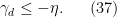
for all bounded measurable functions
on
.
Example 5 (Decoupling for the paraboloid)
into
cubes
of sidelength
. For any
, define the extension operators
and
for
and
. We also introduce the weight function
For any
, let
be the smallest constant for which one has the decoupling inequality
The decoupling theorem of Bourgain and Demeter asserts that
.
![\displaystyle E_{[0,1]^{d-1}} g( x', x_d ) := \int_{[0,1]^{d-1}} e^{2\pi i (x' \cdot \xi + x_d |\xi|^2)} g(\xi)\ d\xi](https://s0.wp.com/latex.php?latex=%5Cdisplaystyle++E_%7B%5B0%2C1%5D%5E%7Bd-1%7D%7D+g%28+x%27%2C+x_d+%29+%3A%3D+%5Cint_%7B%5B0%2C1%5D%5E%7Bd-1%7D%7D+e%5E%7B2%5Cpi+i+%28x%27+%5Ccdot+%5Cxi+%2B+x_d+%7C%5Cxi%7C%5E2%29%7D+g%28%5Cxi%29%5C+d%5Cxi&bg=ffffff&fg=000000&s=0&c=20201002)
![\displaystyle \| E_{[0,1]^{d-1}} g \|_{L^p(w_{B(0,N)})} \leq D_p(N) (\sum_Q \| E_Q g \|_{L^p(w_{B(0,N)})}^2)^{1/2}.](https://s0.wp.com/latex.php?latex=%5Cdisplaystyle++%5C%7C+E_%7B%5B0%2C1%5D%5E%7Bd-1%7D%7D+g+%5C%7C_%7BL%5Ep%28w_%7BB%280%2CN%29%7D%29%7D+%5Cleq+D_p%28N%29+%28%5Csum_Q+%5C%7C+E_Q+g+%5C%7C_%7BL%5Ep%28w_%7BB%280%2CN%29%7D%29%7D%5E2%29%5E%7B1%2F2%7D.&bg=ffffff&fg=000000&s=0&c=20201002)
Example 6 (Decoupling for the moment curve)
into
of length
, define the extension operators
and more generally
for
. For any
It was shown by Bourgain, Demeter, and Guth that
, which among other things implies the Vinogradov main conjecture (as discussed in this previous post).
![\displaystyle E_{[0,1]} g(x_1,\dots,x_d) = \int_{[0,1]} e^{2\pi i ( x_1 \xi + x_2 \xi^2 + \dots + x_d \xi^d} g(\xi)\ d\xi](https://s0.wp.com/latex.php?latex=%5Cdisplaystyle++E_%7B%5B0%2C1%5D%7D+g%28x_1%2C%5Cdots%2Cx_d%29+%3D+%5Cint_%7B%5B0%2C1%5D%7D+e%5E%7B2%5Cpi+i+%28+x_1+%5Cxi+%2B+x_2+%5Cxi%5E2+%2B+%5Cdots+%2B+x_d+%5Cxi%5Ed%7D+g%28%5Cxi%29%5C+d%5Cxi&bg=ffffff&fg=000000&s=0&c=20201002)
![\displaystyle E_J g(x_1,\dots,x_d) = \int_{[0,1]} e^{2\pi i ( x_1 \xi + x_2 \xi^2 + \dots + x_d \xi^d} g(\xi)\ d\xi](https://s0.wp.com/latex.php?latex=%5Cdisplaystyle++E_J+g%28x_1%2C%5Cdots%2Cx_d%29+%3D+%5Cint_%7B%5B0%2C1%5D%7D+e%5E%7B2%5Cpi+i+%28+x_1+%5Cxi+%2B+x_2+%5Cxi%5E2+%2B+%5Cdots+%2B+x_d+%5Cxi%5Ed%7D+g%28%5Cxi%29%5C+d%5Cxi&bg=ffffff&fg=000000&s=0&c=20201002)
![\displaystyle \| E_{[0,1]} g \|_{L^p(w_{B(0,N^d)})} \leq D_p(N) (\sum_J \| E_J g \|_{L^p(w_{B(0,N^d)})}^2)^{1/2}.](https://s0.wp.com/latex.php?latex=%5Cdisplaystyle++%5C%7C+E_%7B%5B0%2C1%5D%7D+g+%5C%7C_%7BL%5Ep%28w_%7BB%280%2CN%5Ed%29%7D%29%7D+%5Cleq+D_p%28N%29+%28%5Csum_J+%5C%7C+E_J+g+%5C%7C_%7BL%5Ep%28w_%7BB%280%2CN%5Ed%29%7D%29%7D%5E2%29%5E%7B1%2F2%7D.&bg=ffffff&fg=000000&s=0&c=20201002)
It is convenient to use asymptotic notation to express these estimates. We write 


while the statement that

and similarly the statement that

Many modern approaches to bounding quantities like 


for all 
for any fixed 
for some constant 
Exercise 7 If
for any fixed
notation is independent of
In more recent years, more sophisticated induction on scales arguments have emerged in which one or more auxiliary quantities besides 


- (Triangle inequality) For any
, we have
- (Multiplicativity) For any
, one has
- (Loomis-Whitney inequality) We have


These inequalities now imply that

and hence by (7) (with 

where the implied constant in the 
Now we give a slightly more sophisticated example, abstracted from the proof of 


- (Crude upper bound for
)
.
- (Bilinear reduction, using parabolic rescaling) For any
- (Crude upper bound for
- (Application of multilinear Kakeya and
decoupling) If
are sufficiently small (e.g. both less than
), then


In all of these bounds the implied constant exponents such as 


It turns out that these estimates imply that 

for all 
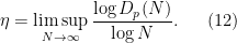
We will call this the upper exponent of 


for any sufficiently small

for any 

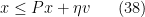
Applying (8) we then have

If we choose 


Exercise 8 Show that one still obtains a subpolynomial upper bound if the estimate (10) is replaced with
for some constant
, so long as we also improve (9) to
(This variant of the argument lets one handle the non-endpoint cases
of the decoupling theorem for the paraboloid.)

To establish decoupling estimates for the moment curve, restricting to the endpoint case 


- (Crude upper bound for
- (Multilinear reduction, using non-isotropic rescaling) For any
- (Crude upper bound for
- (Hölder) For
and
one has
and also
whenever, where
.
- (Rescaled decoupling hypothesis) For
- (Lower dimensional decoupling) If
and
, then
- (Multilinear Kakeya) If
, then


It is now substantially less obvious that these estimates can be combined to demonstrate that
These examples indicate a general strategy to establish that some quantity
- (i) Introducing some family of related auxiliary quantities, often parameterised by several further parameters;
- (ii) establishing as many bounds between these quantities and the original quantity
- (iii) appealing to some sort of “induction on scales” to conclude.
The first two steps (i), (ii) depend very much on the harmonic analysis nature of the quantities
In this post I would like to observe that one can clean up and made more systematic this final step (iii) by passing to upper exponents (12) to eliminate the role of the parameter
For instance, if

from which it is immediate that 
Exercise 9 Repeat Exercise 7 using this method.
Similarly, given the quantities 


for any 


For any natural number 


Now suppose that 


for all 
Assume for contradiction that 

At this point we can eliminate the role of

then on taking limit superiors of the previous inequalities we conclude that

for all 

so that 


This leads to a contradiction when
Exercise 10 Redo Exercise 8 using this method.
The same strategy now clarifies how to proceed with the more complicated system of quantities 


for all

for

for
As before, if we assume for sake of contradiction that

We can then again eliminate the role of 

and thus getting the simplified axiom system


and also

for

for
In view of the latter two estimates it is natural to restrict attention to the quantities 


The axioms now simplify to


 , and
, and 
for
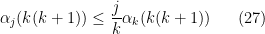
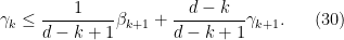
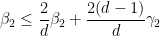
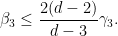
It turns out that the inequality (27) is strongest when 

for
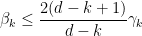
From the last two inequalities (28), (29) we see that a special role is likely to be played by the exponents
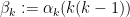
for 
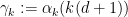
for 

for
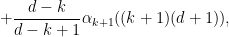
Similarly, from (25) and a brief calculation we have
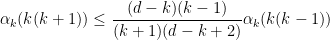

for 


for

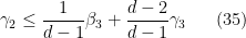
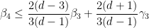
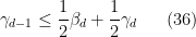
Let us write out the system of equations we have obtained in full:
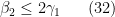
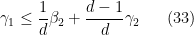
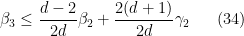


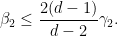
We can then eliminate the variables one by one. Inserting (33) into (32) we obtain
which simplifies to
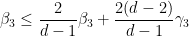
Inserting this into (34) gives

which when combined with (35) gives
which simplifies to
Iterating this we get

for all
for all

which on insertion into (36), (37) gives

which is absurd if
Remark 11 (This observation is essentially due to Heath-Brown.) If we let
denote the column vector with entries
(arranged in whatever order one pleases), then the above system of inequalities (32)–(36) (using (37) to handle the appearance of
in (36)) reads
for some explicit square matrix
with non-negative coefficients, where the inequality denotes pointwise domination, and
is an explicit vector with non-positive coefficients that reflects the effect of (37). It is possible to show (using (24), (26)) that all the coefficients of
for any natural number
would now grow exponentially; this is typically the situation for “non-endpoint” applications such as proving decoupling inequalities away from the endpoint. In the endpoint situation discussed above, the Perron-Frobenius eigenvalue is
now grows at least linearly, which still gives the required contradiction for any
is the spectral radius of
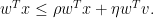
is a left Perron-Frobenius eigenvector, that is to say a non-negative vector, not identically zero, such that
, then by taking inner products of (38) with
we obtain
If
this leads to a contradiction since
is negative and
is non-positive. When
one still gets a contradiction as long as

Remark 12 (This calculation is essentially due to Guo and Zorin-Kranich.) Here is a concrete application of the Perron-Frobenius strategy outlined above to the system of inequalities (32)–(37). Consider the weighted sum
I had secretly calculated the weights
,
as coming from the left Perron-Frobenius eigenvector of the matrix
is bounded by
(with the convention that the
term is absent); this simplifies after some calculation to the bound
and this and (37) then leads to the required contradiction.


Exercise 13
- (i) Extend the above analysis to also cover the non-endpoint case
. (One will need to establish the claim
for
.)
- (ii) Modify the argument to deal with the remaining cases
by dropping some of the steps.

11 comments
Comments feed for this article
14 June, 2019 at 9:32 pm
domotorp
The matching lower bound inequality (2.5) is in the wrong way.
[Corrected, thanks – T.]
14 June, 2019 at 11:17 pm
None
The inequality in (7) seems a bit confusing to me, is the implicit constant a eps power of M instead of N?
[Reworded – T.]
15 June, 2019 at 3:32 am
George Shakan
This reminds me of section 4 of Heath brown’s exposition of Wooley’s proof of the cubic case of efficient congruencing in Vinogradov’s mean value theorem
Click to access 1512.03272.pdf
15 June, 2019 at 7:56 am
Terence Tao
Thanks for pointing this out! In particular Heath-Brown’s observation clarifies exactly when the iteration is “strong enough” to get subpolynomial bounds – one needs the coefficient matrix of the bounds to have an eigenvalue that either exceeds one in magnitude (in which case the iteration grows exponentially), or equals one but has a nontrivial additive component coming from the induction hypothesis (in which case the iteration grows polynomially). I’ve added a remark to this effect.
15 June, 2019 at 1:52 pm
Pavel Zorin-Kranich
For the Bourgain-Demeter-Guth iteration we computed the (right) Perron-Frobenius eigenvector of the matrix of bounds in a paper with Shaoming Guo, see Theorem 3.22 in
https://arxiv.org/abs/1811.02207v1
We also found that making this calculation explicit shortens the argument substantially.
16 June, 2019 at 7:31 am
Terence Tao
Thanks for this! I have added a version of your calculation as an additional remark to the post.
18 June, 2019 at 11:58 pm
Trevor Wooley
This observation that the eigen value should be at least 1 in order to establish the necessary exponential or logarithmic growth required to prove diagonal behaviour in Vinogradov’s mean value theorem also occurs in my own work establishing the cubic case of the main conjecture (arxiv:1401.3150, so January 2014) — this was the paper that Heath-Brown sought to simplify in his own exposition of December 2015. The observation is also critical to my slightly early paper (arxiv:1401.2932) “almost” proving the main conjecture in Vinogradov’s mean value theorem for all degrees, and also in the proof of the main conjecture via nested efficient congruencing. These are all p-adic methods using induction on scales of course, as opposed to real methods (corresponding to p equals infinity).
Incidentally, the first use of different real scales in this subject is due to Vinogradov himself in 1935 in his early work on his mean value theorem, though I suppose this can be traced even to work a decade earlier of Hardy and Littlewood on Waring’s problem.
15 June, 2019 at 6:00 am
Anonymous
Dear Pro.Tao,
Within the 100 years, no mathematician in the world has been expected and inspired like you. You are liked a light of the antique oil lighter, if the light is out, the spirit of math community will be down. We hope you have many progress in attacking problems which have not been solved in many decades yet. In sum, we have some words that sent to you:” Time is gold” . You will understand our idea, because you are very smart.
16 June, 2019 at 6:31 pm
George
really enjoy your article and books
24 June, 2019 at 12:03 pm
Andy
You are still smart. While I am unemployed for a long long time, and I fell I’m getting more and more stupid.
24 June, 2019 at 3:48 pm
Anonymous
C’mon, mate! Cheer up! And please find something to laugh or smile about. And best wishes to you. :-)