
You are currently browsing the tag archive for the ‘decoupling’ tag.
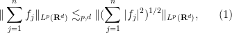
The square root cancellation heuristic, briefly mentioned in the preceding set of notes, predicts that if a collection 
similarly, if 

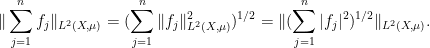
We have already seen one instance in which this heuristic can be made precise, namely when the phases of 
or a reverse square function estimate
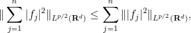
(or both) are known or conjectured to hold. For instance, the useful Littlewood-Paley inequality implies (among other things) that for any 
whenever the Fourier transforms 


if there is some separation between the annuli (for instance if the 


In particular, this identity holds if the 

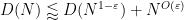
In recent years, it has begun to be realised that in the regime 

(actually in practice we often permit small losses such as 

and taking the square root of both side to conclude that
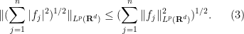
However, the flip side of this weakness is that (2) can be easier to prove. One key reason for this is the ability to iterate decoupling estimates such as (2), in a way that does not seem to be possible with reverse square function estimates such as (1). For instance, suppose that one has a decoupling inequality such as (2), and furthermore each 
Then by inserting these bounds back into (2) we see that we have the combined decoupling inequality

This iterative feature of decoupling inequalities means that such inequalities work well with the method of induction on scales, that we introduced in the previous set of notes.
In fact, decoupling estimates share many features in common with restriction theorems; in addition to induction on scales, there are several other techniques that first emerged in the restriction theory literature, such as wave packet decompositions, rescaling, and bilinear or multilinear reductions, that turned out to also be well suited to proving decoupling estimates. As with restriction, the curvature or transversality of the different Fourier supports of the
Strikingly, in many important model cases, the optimal decoupling inequalities (except possibly for epsilon losses in the exponents) are now known. These estimates have in turn had a number of important applications, such as establishing certain discrete analogues of the restriction conjecture, or the first proof of the main conjecture for Vinogradov mean value theorems in analytic number theory.
These notes only serve as a brief introduction to decoupling. A systematic exploration of this topic can be found in this recent text of Demeter.
Read the rest of this entry »
The following situation is very common in modern harmonic analysis: one has a large scale parameter 


for all 
for all 


in which case the property of having a subpolynomial upper bound is equivalent to that of being subpolynomial size in the sense that

for all
Let us give some illustrative examples of this type of problem:
Example 1 (Kakeya conjecture) Here
be a fixed dimension. For each
, we pick a maximal
-separated set of directions
. We let
where
is a
-tube oriented in the direction
. The Kakeya maximal function conjecture is then equivalent to the assertion that
.
Example 2 (Restriction conjecture for the sphere) Here
for all bounded measurable functions
on the unit sphere
equipped with surface measure
, where
is the ball of radius

Example 3 (Multilinear Kakeya inequality) Again
be compact subsets of the sphere
for the wedge product of directions
for
(equivalently, there is no hyperplane through the origin that intersects all of the
). For each
where for each
is a collection of infinite tubes in
of radius
oriented in a direction in
in
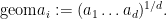
is our notation for the geometric mean
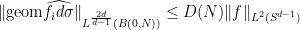
The multilinear Kakeya inequality of Bennett, Carbery, and myself establishes that
Example 4 (Multilinear restriction theorem) Once again
for all bounded measurable functions
on
.
Example 5 (Decoupling for the paraboloid)
into
cubes
of sidelength
. For any
, define the extension operators
and
for
and
. We also introduce the weight function
For any
, let
be the smallest constant for which one has the decoupling inequality
The decoupling theorem of Bourgain and Demeter asserts that
.
![\displaystyle E_{[0,1]^{d-1}} g( x', x_d ) := \int_{[0,1]^{d-1}} e^{2\pi i (x' \cdot \xi + x_d |\xi|^2)} g(\xi)\ d\xi](https://s0.wp.com/latex.php?latex=%5Cdisplaystyle++E_%7B%5B0%2C1%5D%5E%7Bd-1%7D%7D+g%28+x%27%2C+x_d+%29+%3A%3D+%5Cint_%7B%5B0%2C1%5D%5E%7Bd-1%7D%7D+e%5E%7B2%5Cpi+i+%28x%27+%5Ccdot+%5Cxi+%2B+x_d+%7C%5Cxi%7C%5E2%29%7D+g%28%5Cxi%29%5C+d%5Cxi&bg=ffffff&fg=000000&s=0&c=20201002)
![\displaystyle \| E_{[0,1]^{d-1}} g \|_{L^p(w_{B(0,N)})} \leq D_p(N) (\sum_Q \| E_Q g \|_{L^p(w_{B(0,N)})}^2)^{1/2}.](https://s0.wp.com/latex.php?latex=%5Cdisplaystyle++%5C%7C+E_%7B%5B0%2C1%5D%5E%7Bd-1%7D%7D+g+%5C%7C_%7BL%5Ep%28w_%7BB%280%2CN%29%7D%29%7D+%5Cleq+D_p%28N%29+%28%5Csum_Q+%5C%7C+E_Q+g+%5C%7C_%7BL%5Ep%28w_%7BB%280%2CN%29%7D%29%7D%5E2%29%5E%7B1%2F2%7D.&bg=ffffff&fg=000000&s=0&c=20201002)
Example 6 (Decoupling for the moment curve)
into
of length
, define the extension operators
and more generally
for
. For any
It was shown by Bourgain, Demeter, and Guth that
, which among other things implies the Vinogradov main conjecture (as discussed in this previous post).
![\displaystyle E_{[0,1]} g(x_1,\dots,x_d) = \int_{[0,1]} e^{2\pi i ( x_1 \xi + x_2 \xi^2 + \dots + x_d \xi^d} g(\xi)\ d\xi](https://s0.wp.com/latex.php?latex=%5Cdisplaystyle++E_%7B%5B0%2C1%5D%7D+g%28x_1%2C%5Cdots%2Cx_d%29+%3D+%5Cint_%7B%5B0%2C1%5D%7D+e%5E%7B2%5Cpi+i+%28+x_1+%5Cxi+%2B+x_2+%5Cxi%5E2+%2B+%5Cdots+%2B+x_d+%5Cxi%5Ed%7D+g%28%5Cxi%29%5C+d%5Cxi&bg=ffffff&fg=000000&s=0&c=20201002)
![\displaystyle E_J g(x_1,\dots,x_d) = \int_{[0,1]} e^{2\pi i ( x_1 \xi + x_2 \xi^2 + \dots + x_d \xi^d} g(\xi)\ d\xi](https://s0.wp.com/latex.php?latex=%5Cdisplaystyle++E_J+g%28x_1%2C%5Cdots%2Cx_d%29+%3D+%5Cint_%7B%5B0%2C1%5D%7D+e%5E%7B2%5Cpi+i+%28+x_1+%5Cxi+%2B+x_2+%5Cxi%5E2+%2B+%5Cdots+%2B+x_d+%5Cxi%5Ed%7D+g%28%5Cxi%29%5C+d%5Cxi&bg=ffffff&fg=000000&s=0&c=20201002)
![\displaystyle \| E_{[0,1]} g \|_{L^p(w_{B(0,N^d)})} \leq D_p(N) (\sum_J \| E_J g \|_{L^p(w_{B(0,N^d)})}^2)^{1/2}.](https://s0.wp.com/latex.php?latex=%5Cdisplaystyle++%5C%7C+E_%7B%5B0%2C1%5D%7D+g+%5C%7C_%7BL%5Ep%28w_%7BB%280%2CN%5Ed%29%7D%29%7D+%5Cleq+D_p%28N%29+%28%5Csum_J+%5C%7C+E_J+g+%5C%7C_%7BL%5Ep%28w_%7BB%280%2CN%5Ed%29%7D%29%7D%5E2%29%5E%7B1%2F2%7D.&bg=ffffff&fg=000000&s=0&c=20201002)
It is convenient to use asymptotic notation to express these estimates. We write 


while the statement that

and similarly the statement that

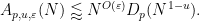
Many modern approaches to bounding quantities like 


for all 
for any fixed 
for some constant 
Exercise 7 If
for any fixed
notation is independent of
In more recent years, more sophisticated induction on scales arguments have emerged in which one or more auxiliary quantities besides 


- (Triangle inequality) For any
, we have
- (Multiplicativity) For any
, one has
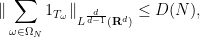
- (Loomis-Whitney inequality) We have


These inequalities now imply that

and hence by (7) (with 

where the implied constant in the 
Now we give a slightly more sophisticated example, abstracted from the proof of 


- (Crude upper bound for
)
.
- (Bilinear reduction, using parabolic rescaling) For any
- (Crude upper bound for
- (Application of multilinear Kakeya and
decoupling) If
are sufficiently small (e.g. both less than
), then


In all of these bounds the implied constant exponents such as 


It turns out that these estimates imply that 

for all 
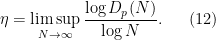
We will call this the upper exponent of 


for any sufficiently small

for any 

Applying (8) we then have

If we choose 


Exercise 8 Show that one still obtains a subpolynomial upper bound if the estimate (10) is replaced with
for some constant
, so long as we also improve (9) to
(This variant of the argument lets one handle the non-endpoint cases
of the decoupling theorem for the paraboloid.)

To establish decoupling estimates for the moment curve, restricting to the endpoint case 


- (Crude upper bound for
- (Multilinear reduction, using non-isotropic rescaling) For any
- (Crude upper bound for
- (Hölder) For
and
one has
and also
whenever, where
.
- (Rescaled decoupling hypothesis) For
- (Lower dimensional decoupling) If
and
, then
- (Multilinear Kakeya) If
, then


It is now substantially less obvious that these estimates can be combined to demonstrate that
These examples indicate a general strategy to establish that some quantity
- (i) Introducing some family of related auxiliary quantities, often parameterised by several further parameters;
- (ii) establishing as many bounds between these quantities and the original quantity
- (iii) appealing to some sort of “induction on scales” to conclude.
The first two steps (i), (ii) depend very much on the harmonic analysis nature of the quantities
In this post I would like to observe that one can clean up and made more systematic this final step (iii) by passing to upper exponents (12) to eliminate the role of the parameter
For instance, if

from which it is immediate that 
Exercise 9 Repeat Exercise 7 using this method.
Similarly, given the quantities 


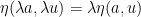
for any 


For any natural number 


Now suppose that 


for all 
Assume for contradiction that 

At this point we can eliminate the role of

then on taking limit superiors of the previous inequalities we conclude that

for all 

so that 


This leads to a contradiction when
Exercise 10 Redo Exercise 8 using this method.
The same strategy now clarifies how to proceed with the more complicated system of quantities 


for all

for

for
As before, if we assume for sake of contradiction that

We can then again eliminate the role of 

and thus getting the simplified axiom system


and also

for

for
In view of the latter two estimates it is natural to restrict attention to the quantities 


The axioms now simplify to


 , and
, and 
for
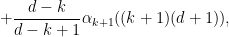
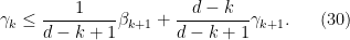
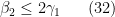
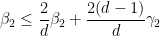
It turns out that the inequality (27) is strongest when 

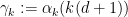
for
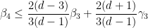
From the last two inequalities (28), (29) we see that a special role is likely to be played by the exponents
for 
for 

for
Similarly, from (25) and a brief calculation we have

for 


for

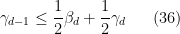
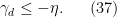
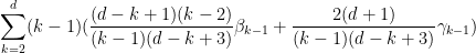
Let us write out the system of equations we have obtained in full:
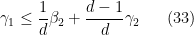


We can then eliminate the variables one by one. Inserting (33) into (32) we obtain
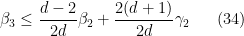
which simplifies to
Inserting this into (34) gives

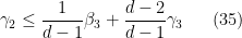
which when combined with (35) gives
which simplifies to
Iterating this we get

for all
for all

which on insertion into (36), (37) gives

which is absurd if
Remark 11 (This observation is essentially due to Heath-Brown.) If we let
denote the column vector with entries
(arranged in whatever order one pleases), then the above system of inequalities (32)–(36) (using (37) to handle the appearance of
in (36)) reads
for some explicit square matrix
with non-negative coefficients, where the inequality denotes pointwise domination, and
is an explicit vector with non-positive coefficients that reflects the effect of (37). It is possible to show (using (24), (26)) that all the coefficients of
for any natural number
would now grow exponentially; this is typically the situation for “non-endpoint” applications such as proving decoupling inequalities away from the endpoint. In the endpoint situation discussed above, the Perron-Frobenius eigenvalue is
now grows at least linearly, which still gives the required contradiction for any
is the spectral radius of
is a left Perron-Frobenius eigenvector, that is to say a non-negative vector, not identically zero, such that
, then by taking inner products of (38) with
we obtain
If
this leads to a contradiction since
is negative and
is non-positive. When
one still gets a contradiction as long as

Remark 12 (This calculation is essentially due to Guo and Zorin-Kranich.) Here is a concrete application of the Perron-Frobenius strategy outlined above to the system of inequalities (32)–(37). Consider the weighted sum
I had secretly calculated the weights
,
as coming from the left Perron-Frobenius eigenvector of the matrix
is bounded by
(with the convention that the
term is absent); this simplifies after some calculation to the bound
and this and (37) then leads to the required contradiction.


Exercise 13
- (i) Extend the above analysis to also cover the non-endpoint case
. (One will need to establish the claim
for
.)
- (ii) Modify the argument to deal with the remaining cases
by dropping some of the steps.
In this blog post, I would like to specialise the arguments of Bourgain, Demeter, and Guth from the previous post to the two-dimensional case of the Vinogradov main conjecture, namely
Theorem 1 (Two-dimensional Vinogradov main conjecture) One has
as
![\displaystyle \int_{[0,1]^2} |\sum_{j=0}^N e( j x + j^2 y)|^6\ dx dy \ll N^{3+o(1)}](https://s0.wp.com/latex.php?latex=%5Cdisplaystyle++%5Cint_%7B%5B0%2C1%5D%5E2%7D+%7C%5Csum_%7Bj%3D0%7D%5EN+e%28+j+x+%2B+j%5E2+y%29%7C%5E6%5C+dx+dy+%5Cll+N%5E%7B3%2Bo%281%29%7D&bg=ffffff&fg=000000&s=0&c=20201002)
This particular case of the main conjecture has a classical proof using some elementary number theory. Indeed, the left-hand side can be viewed as the number of solutions to the system of equations


with 


which, when combined with the divisor bound, shows that each 


In this special case, the Bourgain-Demeter argument simplifies, as the lower dimensional inductive hypothesis becomes a simple
We now give the specialisation of the Bourgain-Demeter argument to Theorem 1. It will suffice to establish the bound
![\displaystyle \int_{[0,1]^2} |\sum_{j=0}^N e( j x + j^2 y)|^p\ dx dy \ll N^{p/2+o(1)}](https://s0.wp.com/latex.php?latex=%5Cdisplaystyle++%5Cint_%7B%5B0%2C1%5D%5E2%7D+%7C%5Csum_%7Bj%3D0%7D%5EN+e%28+j+x+%2B+j%5E2+y%29%7C%5Ep%5C+dx+dy+%5Cll+N%5E%7Bp%2F2%2Bo%281%29%7D&bg=ffffff&fg=000000&s=0&c=20201002)
for all 


![\displaystyle \int_{[0,1]^2} |\sum_{j=0}^N e( j x + j^2 y)|^p\ dx dy \ll N^{p/2+\eta+o(1)}](https://s0.wp.com/latex.php?latex=%5Cdisplaystyle++%5Cint_%7B%5B0%2C1%5D%5E2%7D+%7C%5Csum_%7Bj%3D0%7D%5EN+e%28+j+x+%2B+j%5E2+y%29%7C%5Ep%5C+dx+dy+%5Cll+N%5E%7Bp%2F2%2B%5Ceta%2Bo%281%29%7D&bg=ffffff&fg=000000&s=0&c=20201002)
as
Proposition 2 Let
(with
holds.
Indeed, this proposition shows that for
We prove the proposition below the fold, using a simplified form of the methods discussed in the previous blog post. To simplify the exposition we will be a bit cavalier with the uncertainty principle, for instance by essentially ignoring the tails of rapidly decreasing functions.
Given any finite collection of elements 

However, when the
For sake of comparison, from the triangle inequality and Cauchy-Schwarz one has the general inequality
for any finite collection 


More generally, let us somewhat informally say that a collection
for any 


and the right-hand side can be much larger than 

However, in some cases one can get decoupling for certain 


giving decoupling in 


In recent years, Bourgain and Demeter have been establishing decoupling theorems in 


For any ball 


which should be viewed as a smoothed out version of the indicator function 


![{\gamma([0,1])}](https://s0.wp.com/latex.php?latex=%7B%5Cgamma%28%5B0%2C1%5D%29%7D&bg=ffffff&fg=000000&s=0&c=20201002)
Theorem 1 (Decoupling theorem) Let
. Subdivide the unit interval
of length
be the Fourier transform
of a finite Borel measure
on the arc
, where
. Then the
for any ball
.
Orthogonality gives the 


where 


On the other hand, 


This theorem has the following consequence of importance in analytic number theory:
Corollary 2 (Vinogradov main conjecture) Let
be integers, and let
. Then
![\displaystyle \int_{[0,1]^n} |\sum_{j=1}^N e( j x_1 + j^2 x_2 + \dots + j^n x_n)|^{2s}\ dx_1 \dots dx_n](https://s0.wp.com/latex.php?latex=%5Cdisplaystyle+%5Cint_%7B%5B0%2C1%5D%5En%7D+%7C%5Csum_%7Bj%3D1%7D%5EN+e%28+j+x_1+%2B+j%5E2+x_2+%2B+%5Cdots+%2B+j%5En+x_n%29%7C%5E%7B2s%7D%5C+dx_1+%5Cdots+dx_n+&bg=ffffff&fg=000000&s=0&c=20201002)
Proof: By the Hölder inequality (and the trivial bound of 
![\displaystyle \int_{[0,1]^n} |\sum_{j=1}^N e( j x_1 + j^2 x_2 + \dots + j^n x_n)|^{n(n+1)}\ dx_1 \dots dx_n \ll_{\varepsilon,n} N^{\frac{n(n+1)}{2}+\varepsilon}.](https://s0.wp.com/latex.php?latex=%5Cdisplaystyle+%5Cint_%7B%5B0%2C1%5D%5En%7D+%7C%5Csum_%7Bj%3D1%7D%5EN+e%28+j+x_1+%2B+j%5E2+x_2+%2B+%5Cdots+%2B+j%5En+x_n%29%7C%5E%7Bn%28n%2B1%29%7D%5C+dx_1+%5Cdots+dx_n+%5Cll_%7B%5Cvarepsilon%2Cn%7D+N%5E%7B%5Cfrac%7Bn%28n%2B1%29%7D%7B2%7D%2B%5Cvarepsilon%7D.&bg=ffffff&fg=000000&s=0&c=20201002)
We can rescale this as
![\displaystyle \int_{[0,N] \times [0,N^2] \times \dots \times [0,N^n]} |\sum_{j=1}^N e( x \cdot \gamma(j/N) )|^{n(n+1)}\ dx \ll_{\varepsilon,n} N^{n(n+1)+\varepsilon}.](https://s0.wp.com/latex.php?latex=%5Cdisplaystyle+%5Cint_%7B%5B0%2CN%5D+%5Ctimes+%5B0%2CN%5E2%5D+%5Ctimes+%5Cdots+%5Ctimes+%5B0%2CN%5En%5D%7D+%7C%5Csum_%7Bj%3D1%7D%5EN+e%28+x+%5Ccdot+%5Cgamma%28j%2FN%29+%29%7C%5E%7Bn%28n%2B1%29%7D%5C+dx+%5Cll_%7B%5Cvarepsilon%2Cn%7D+N%5E%7Bn%28n%2B1%29%2B%5Cvarepsilon%7D.&bg=ffffff&fg=000000&s=0&c=20201002)
As the integrand is periodic along the lattice 
![\displaystyle \int_{[0,N^n]^n} |\sum_{j=1}^N e( x \cdot \gamma(j/N) )|^{n(n+1)}\ dx \ll_{\varepsilon,n} N^{\frac{n(n+1)}{2}+n^2+\varepsilon}.](https://s0.wp.com/latex.php?latex=%5Cdisplaystyle+%5Cint_%7B%5B0%2CN%5En%5D%5En%7D+%7C%5Csum_%7Bj%3D1%7D%5EN+e%28+x+%5Ccdot+%5Cgamma%28j%2FN%29+%29%7C%5E%7Bn%28n%2B1%29%7D%5C+dx+%5Cll_%7B%5Cvarepsilon%2Cn%7D+N%5E%7B%5Cfrac%7Bn%28n%2B1%29%7D%7B2%7D%2Bn%5E2%2B%5Cvarepsilon%7D.&bg=ffffff&fg=000000&s=0&c=20201002)
The left-hand side may be bounded by 


the claim now follows from the decoupling theorem and a brief calculation.

Using the Plancherel formula, one may equivalently (when 


but we will not use this formulation here.
A history of the Vinogradov main conjecture may be found in this survey of Wooley; prior to the Bourgain-Demeter-Guth theorem, the conjecture was solved completely for 


Below the fold we sketch the Bourgain-Demeter-Guth argument proving Theorem 1.
I thank Jean Bourgain and Andrew Granville for helpful discussions.

Recent Comments