
You are currently browsing the tag archive for the ‘quantum mechanics’ tag.
In contrast to previous notes, in this set of notes we shall focus exclusively on Fourier analysis in the one-dimensional setting 

In previous notes we have often performed various localisations in either physical space or Fourier space 
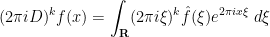
and the momentum operator 
(The terminology comes from quantum mechanics, where it is customary to also insert a small constant 


for any 


for all 

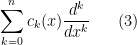
Clearly, for any polynomial 


and similarly the operator 
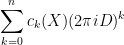
Inspired by this, if 
for all 


one can easily verify from several applications of the Leibniz rule that 


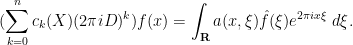
For instance, any constant coefficient linear differential operators 
however there are many Fourier multiplier operators that are not of this form, such as fractional derivative operators 


We observe that the maps 


and

for any 


for 
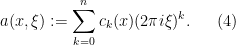
In the field of PDE and ODE, it is also very common to study variable coefficient linear differential operators
where the 

and so it is natural to interpret this operator as a combination 


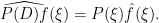
Indeed, from the Fourier inversion formula
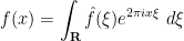
for any
and hence on multiplying by 
Inspired by this, we can introduce the Kohn-Nirenberg quantisation by defining the operator 
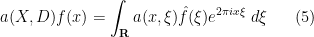
whenever
for all 


 are two functions obeying
  for all
  . (Hint: apply
  to a suitable truncation of a plane wave
  and then take limits.)
In principle, the quantisations 

in general. Fundamentally, this is due to the fact that pointwise multiplication of symbols is a commutative operation, whereas the composition of operators such as
![\displaystyle [A,B] := AB - BA](https://s0.wp.com/latex.php?latex=%5Cdisplaystyle++%5BA%2CB%5D+%3A%3D+AB+-+BA&bg=ffffff&fg=000000&s=0&c=20201002)
of two operators 
![\displaystyle [X,D] = -\frac{1}{2\pi i} \neq 0.](https://s0.wp.com/latex.php?latex=%5Cdisplaystyle++%5BX%2CD%5D+%3D+-%5Cfrac%7B1%7D%7B2%5Cpi+i%7D+%5Cneq+0.&bg=ffffff&fg=000000&s=0&c=20201002)
(In the language of Lie groups and Lie algebras, this tells us that
Exercise 2 (Heisenberg uncertainty principle) For any
and
, show that
(Hint: evaluate the expression
in two different ways and apply the Cauchy-Schwarz inequality.) Informally, this exercise asserts that the spatial uncertainty
and the frequency uncertainty
of a function obey the Heisenberg uncertainty relation
.

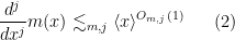
Nevertheless, one still has the correspondence principle, which asserts that in certain regimes (which, with our choice of normalisations, corresponds to the high-frequency regime), quantum mechanics continues to behave like a commutative theory, and one can sometimes proceed as if the operators

where the error between the left and right-hand sides is of “lower order” and can in fact enjoys a useful asymptotic expansion. As a first approximation to this calculus, one can think of functions 


Unfortunately the uncertainty principle (or the non-commutativity of 

To complement the pseudodifferential calculus we have the basic Calderón-Vaillancourt theorem, which asserts that pseudodifferential operators of order zero are Calderón-Zygmund operators and thus bounded on 

Pseudodifferential operators (especially when generalised to higher dimensions 
This set of notes is only the briefest introduction to the theory of pseudodifferential operators. Many texts are available that cover the theory in more detail, for instance this text of Taylor.
is the fundamental equation of motion for (non-relativistic) quantum mechanics, modeling both one-particle systems and 


I recently attended a talk by Natasa Pavlovic on the rigorous derivation of this type of limiting behaviour, which was initiated by the pioneering work of Hepp and Spohn, and has now attracted a vast recent literature. The rigorous details here are rather sophisticated; but the heuristic explanation of the phenomenon is fairly simple, and actually rather pretty in my opinion, involving the foundational quantum mechanics of
This discussion will be purely formal, in the sense that (important) analytic issues such as differentiability, existence and uniqueness, etc. will be largely ignored.
My penultimate article for my PCM series is a very short one, on “Hamiltonians“. The PCM has a number of short articles to define terms which occur frequently in the longer articles, but are not substantive enough topics by themselves to warrant a full-length treatment. One of these is the term “Hamiltonian”, which is used in all the standard types of physical mechanics (classical or quantum, microscopic or statistical) to describe the total energy of a system. It is a remarkable feature of the laws of physics that this single object (which is a scalar-valued function in classical physics, and a self-adjoint operator in quantum mechanics) suffices to describe the entire dynamics of a system, although from a mathematical perspective it is not always easy to read off all the analytic aspects of this dynamics just from the form of the Hamiltonian.
In mathematics, Hamiltonians of course arise in the equations of mathematical physics (such as Hamilton’s equations of motion, or Schrödinger’s equations of motion), but also show up in symplectic geometry (as a special case of a moment map) and in microlocal analysis.
For this post, I would also like to highlight an article of my good friend Andrew Granville on one of my own favorite topics, “Analytic number theory“, focusing in particular on the classical problem of understanding the distribution of the primes, via such analytic tools as zeta functions and L-functions, sieve theory, and the circle method.
This post is derived from an interesting conversation I had several years ago with my friend Jason Newquist on trying to find some intuitive analogies for the non-classical nature of quantum mechanics. It occurred to me that this type of informal, rambling discussion might actually be rather suited to the blog medium, so here goes nothing…
Quantum mechanics has a number of weird consequences, but here we are focusing on three (inter-related) ones:
- Objects can behave both like particles (with definite position and a continuum of states) and waves (with indefinite position and (in confined situations) quantised states);
- The equations that govern quantum mechanics are deterministic, but the standard interpretation of the solutions of these equations is probabilistic; and
- If instead one applies the laws of quantum mechanics literally at the macroscopic scale, then the universe itself must split into the superposition of many distinct “worlds”.
In trying to come up with a classical conceptual model in which to capture these non-classical phenomena, we eventually hit upon using the idea of using computer games as an analogy. The exact choice of game is not terribly important, but let us pick Tomb Raider – a popular game from about ten years ago (back when I had the leisure to play these things), in which the heroine, Lara Croft, explores various tombs and dungeons, solving puzzles and dodging traps, in order to achieve some objective. It is quite common for Lara to die in the game, for instance by failing to evade one of the traps. (I should warn that this analogy will be rather violent on certain computer-generated characters.)

Recent Comments