Exploring the toolkit of Jean Bourgain

I have uploaded to the arXiv my paper “Exploring the toolkit of Jean Bourgain“. This is one of a collection of papers to be published in the Bulletin of the American Mathematical Society describing aspects of the work of Jean Bourgain; other contributors to this collection include Keith Ball, Ciprian Demeter, and Carlos Kenig. Because the other contributors will be covering specific areas of Jean’s work in some detail, I decided to take a non-overlapping tack, and focus instead on some basic tools of Jean that he frequently used across many of the fields he contributed to. Jean had a surprising number of these “basic tools” that he wielded with great dexterity, and in this paper I focus on just a few of them:

• Reducing qualitative analysis results (e.g., convergence theorems or dimension bounds) to quantitative analysis estimates (e.g., variational inequalities or maximal function estimates).
• Using dyadic pigeonholing to locate good scales to work in or to apply truncations.
• Using random translations to amplify small sets (low density) into large sets (positive density).
• Combining large deviation inequalities with metric entropy bounds to control suprema of various random processes.

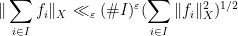
Each of these techniques is individually not too difficult to explain, and were certainly employed on occasion by various mathematicians prior to Bourgain’s work; but Jean had internalized them to the point where he would instinctively use them as soon as they became relevant to a given problem at hand. I illustrate this at the end of the paper with an exposition of one particular result of Jean, on the Erdős similarity problem, in which his main result (that any sum of three infinite sets of reals has the property that there exists a positive measure set that does not contain any homothetic copy of ) is basically proven by a sequential application of these tools (except for dyadic pigeonholing, which turns out not to be needed here).

I had initially intended to also cover some other basic tools in Jean’s toolkit, such as the uncertainty principle and the use of probabilistic decoupling, but was having trouble keeping the paper coherent with such a broad focus (certainly I could not identify a single paper of Jean’s that employed all of these tools at once). I hope though that the examples given in the paper gives some reasonable impression of Jean’s research style.

Decoupling and the Bourgain-Demeter-Guth proof of the Vinogradov main conjecture

Given any finite collection of elements in some Banach space , the triangle inequality tells us that

However, when the all “oscillate in different ways”, one expects to improve substantially upon the triangle inequality. For instance, if is a Hilbert space and the are mutually orthogonal, we have the Pythagorean theorem

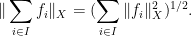
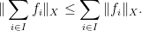
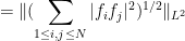
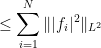
For sake of comparison, from the triangle inequality and Cauchy-Schwarz one has the general inequality

 

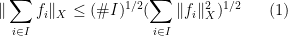
for any finite collection in any Banach space , where denotes the cardinality of . Thus orthogonality in a Hilbert space yields “square root cancellation”, saving a factor of or so over the trivial bound coming from the triangle inequality.

More generally, let us somewhat informally say that a collection exhibits decoupling in if one has the Pythagorean-like inequality

for any , thus one obtains almost the full square root cancellation in the norm. The theory of almost orthogonality can then be viewed as the theory of decoupling in Hilbert spaces such as . In spaces for one usually does not expect this sort of decoupling; for instance, if the are disjointly supported one has

and the right-hand side can be much larger than when . At the opposite extreme, one usually does not expect to get decoupling in , since one could conceivably align the to all attain a maximum magnitude at the same location with the same phase, at which point the triangle inequality in becomes sharp.

However, in some cases one can get decoupling for certain . For instance, suppose we are in , and that are bi-orthogonal in the sense that the products for are pairwise orthogonal in . Then we have

giving decoupling in . (Similarly if each of the is orthogonal to all but of the other .) A similar argument also gives decoupling when one has tri-orthogonality (with the mostly orthogonal to each other), and so forth. As a slight variant, Khintchine’s inequality also indicates that decoupling should occur for any fixed if one multiplies each of the by an independent random sign .

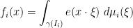
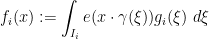
In recent years, Bourgain and Demeter have been establishing decoupling theorems in spaces for various key exponents of , in the “restriction theory” setting in which the are Fourier transforms of measures supported on different portions of a given surface or curve; this builds upon the earlier decoupling theorems of Wolff. In a recent paper with Guth, they established the following decoupling theorem for the curve parameterised by the polynomial curve

For any ball in , let denote the weight

which should be viewed as a smoothed out version of the indicator function of . In particular, the space can be viewed as a smoothed out version of the space . For future reference we observe a fundamental self-similarity of the curve : any arc in this curve, with a compact interval, is affinely equivalent to the standard arc .

Theorem 1 (Decoupling theorem) Let . Subdivide the unit interval into equal subintervals of length , and for each such , let be the Fourier transform

of a finite Borel measure on the arc , where . Then the exhibit decoupling in for any ball of radius .

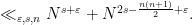
Orthogonality gives the case of this theorem. The bi-orthogonality type arguments sketched earlier only give decoupling in up to the range ; the point here is that we can now get a much larger value of . The case of this theorem was previously established by Bourgain and Demeter (who obtained in fact an analogous theorem for any curved hypersurface). The exponent (and the radius ) is best possible, as can be seen by the following basic example. If

where is a bump function adapted to , then standard Fourier-analytic computations show that will be comparable to on a rectangular box of dimensions (and thus volume ) centred at the origin, and exhibit decay away from this box, with comparable to

On the other hand, is comparable to on a ball of radius comparable to centred at the origin, so is , which is just barely consistent with decoupling. This calculation shows that decoupling will fail if is replaced by any larger exponent, and also if the radius of the ball is reduced to be significantly smaller than .

This theorem has the following consequence of importance in analytic number theory:

Corollary 2 (Vinogradov main conjecture) Let be integers, and let . Then

Proof: By the Hölder inequality (and the trivial bound of for the exponential sum), it suffices to treat the critical case , that is to say to show that

We can rescale this as

As the integrand is periodic along the lattice , this is equivalent to

The left-hand side may be bounded by , where and . Since

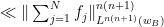
the claim now follows from the decoupling theorem and a brief calculation.

Using the Plancherel formula, one may equivalently (when is an integer) write the Vinogradov main conjecture in terms of solutions to the system of equations

but we will not use this formulation here.

A history of the Vinogradov main conjecture may be found in this survey of Wooley; prior to the Bourgain-Demeter-Guth theorem, the conjecture was solved completely for , or for and either below or above , with the bulk of recent progress coming from the efficient congruencing technique of Wooley. It has numerous applications to exponential sums, Waring’s problem, and the zeta function; to give just one application, the main conjecture implies the predicted asymptotic for the number of ways to express a large number as the sum of fifth powers (the previous best result required fifth powers). The Bourgain-Demeter-Guth approach to the Vinogradov main conjecture, based on decoupling, is ostensibly very different from the efficient congruencing technique, which relies heavily on the arithmetic structure of the program, but it appears (as I have been told from second-hand sources) that the two methods are actually closely related, with the former being a sort of “Archimedean” version of the latter (with the intervals in the decoupling theorem being analogous to congruence classes in the efficient congruencing method); hopefully there will be some future work making this connection more precise. One advantage of the decoupling approach is that it generalises to non-arithmetic settings in which the set that is drawn from is replaced by some other similarly separated set of real numbers. (A random thought – could this allow the Vinogradov-Korobov bounds on the zeta function to extend to Beurling zeta functions?)

Below the fold we sketch the Bourgain-Demeter-Guth argument proving Theorem 1.

I thank Jean Bourgain and Andrew Granville for helpful discussions.

The Katai-Bourgain-Sarnak-Ziegler orthogonality criterion

One of the basic problems in analytic number theory is to estimate sums of the form

as , where ranges over primes and is some explicit function of interest (e.g. a linear phase function for some real number ). This is essentially the same task as obtaining estimates on the sum

where is the von Mangoldt function. If is bounded, , then from the prime number theorem one has the trivial bound

but often (when is somehow “oscillatory” in nature) one is seeking the refinement

or equivalently

Thanks to identities such as

where is the Möbius function, refinements such as (1) are similar in spirit to estimates of the form

Unfortunately, the connection between (1) and (4) is not particularly tight; roughly speaking, one needs to improve the bounds in (4) (and variants thereof) by about two factors of before one can use identities such as (3) to recover (1). Still, one generally thinks of (1) and (4) as being “morally” equivalent, even if they are not formally equivalent.

When is oscillating in a sufficiently “irrational” way, then one standard way to proceed is the method of Type I and Type II sums, which uses truncated versions of divisor identities such as (3) to expand out either (1) or (4) into linear (Type I) or bilinear sums (Type II) with which one can exploit the oscillation of . For instance, Vaughan’s identity lets one rewrite the sum in (1) as the sum of the Type I sum

the Type I sum

the Type II sum

and the error term , whenever are parameters, and are the sequences

and

Similarly one can express (4) as the Type I sum

the Type II sum

and the error term , whenever with , and is the sequence

After eliminating troublesome sequences such as via Cauchy-Schwarz or the triangle inequality, one is then faced with the task of estimating Type I sums such as

or Type II sums such as

for various . Here, the trivial bound is , but due to a number of logarithmic inefficiencies in the above method, one has to obtain bounds that are more like for some constant (e.g. ) in order to end up with an asymptotic such as (1) or (4).

However, in a recent paper of Bourgain, Sarnak, and Ziegler, it was observed that as long as one is only seeking the Mobius orthogonality (4) rather than the von Mangoldt orthogonality (1), one can avoid losing any logarithmic factors, and rely purely on qualitative equidistribution properties of . A special case of their orthogonality criterion (which actually dates back to an earlier paper of Katai, as was pointed out to me by Nikos Frantzikinakis) is as follows:

Proposition 1 (Orthogonality criterion) Let be a bounded function such that

for any distinct primes (where the decay rate of the error term may depend on and ). Then

Actually, the Bourgain-Sarnak-Ziegler paper establishes a more quantitative version of this proposition, in which can be replaced by an arbitrary bounded multiplicative function, but we will content ourselves with the above weaker special case. (See also these notes of Harper, which uses the Katai argument to give a slightly weaker quantitative bound in the same spirit.) This criterion can be viewed as a multiplicative variant of the classical van der Corput lemma, which in our notation asserts that if one has for each fixed non-zero .

As a sample application, Proposition 1 easily gives a proof of the asymptotic

for any irrational . (For rational , this is a little trickier, as it is basically equivalent to the prime number theorem in arithmetic progressions.) The paper of Bourgain, Sarnak, and Ziegler also apply this criterion to nilsequences (obtaining a quick proof of a qualitative version of a result of Ben Green and myself, see these notes of Ziegler for details) and to horocycle flows (for which no Möbius orthogonality result was previously known).

Informally, the connection between (5) and (6) comes from the multiplicative nature of the Möbius function. If (6) failed, then exhibits strong correlation with ; by change of variables, we then expect to correlate with and to correlate with , for “typical” at least. On the other hand, since is multiplicative, exhibits strong correlation with . Putting all this together (and pretending correlation is transitive), this would give the claim (in the contrapositive). Of course, correlation is not quite transitive, but it turns out that one can use the Cauchy-Schwarz inequality as a substitute for transitivity of correlation in this case.

I will give a proof of Proposition 1 below the fold (which is not quite based on the argument in the above mentioned paper, but on a variant of that argument communicated to me by Tamar Ziegler, and also independently discovered by Adam Harper). The main idea is to exploit the following observation: if is a “large” but finite set of primes (in the sense that the sum is large), then for a typical large number (much larger than the elements of ), the number of primes in that divide is pretty close to :

A more precise formalisation of this heuristic is provided by the Turan-Kubilius inequality, which is proven by a simple application of the second moment method.

In particular, one can sum (7) against and obtain an approximation

that approximates a sum of by a bunch of sparser sums of . Since

we see (heuristically, at least) that in order to establish (4), it would suffice to establish the sparser estimates

for all (or at least for “most” ).

Now we make the change of variables . As the Möbius function is multiplicative, we usually have . (There is an exception when is divisible by , but this will be a rare event and we will be able to ignore it.) So it should suffice to show that

for most . However, by the hypothesis (5), the sequences are asymptotically orthogonal as varies, and this claim will then follow from a Cauchy-Schwarz argument.

The Bourgain-Guth argument for proving restriction theorems

One of my favourite unsolved problems in harmonic analysis is the restriction problem. This problem, first posed explicitly by Elias Stein, can take many equivalent forms, but one of them is this: one starts with a smooth compact hypersurface (possibly with boundary) in , such as the unit sphere in , and equips it with surface measure . One then takes a bounded measurable function on this surface, and then computes the (inverse) Fourier transform

of the measure . As is bounded and is a finite measure, this is a bounded function on ; from the dominated convergence theorem, it is also continuous. The restriction problem asks whether this Fourier transform also decays in space, and specifically whether lies in for some . (This is a natural space to control decay because it is translation invariant, which is compatible on the frequency space side with the modulation invariance of .) By the closed graph theorem, this is the case if and only if there is an estimate of the form

for some constant that can depend on but not on . By a limiting argument, to provide such an estimate, it suffices to prove such an estimate under the additional assumption that is smooth.

Strictly speaking, the above problem should be called the extension problem, but it is dual to the original formulation of the restriction problem, which asks to find those exponents for which the Fourier transform of an function can be meaningfully restricted to a hypersurface , in the sense that the map can be continuously defined from to, say, . A duality argument shows that the exponents for which the restriction property holds are the dual exponents to the exponents for which the extension problem holds.

There are several motivations for studying the restriction problem. The problem is connected to the classical question of determining the nature of the convergence of various Fourier summation methods (and specifically, Bochner-Riesz summation); very roughly speaking, if one wishes to perform a partial Fourier transform by restricting the frequencies (possibly using a well-chosen weight) to some region (such as a ball), then one expects this operation to well behaved if the boundary of this region has good restriction (or extension) properties. More generally, the restriction problem for a surface is connected to the behaviour of Fourier multipliers whose symbols are singular at . The problem is also connected to the analysis of various linear PDE such as the Helmholtz equation, Schro\”dinger equation, wave equation, and the (linearised) Korteweg-de Vries equation, because solutions to such equations can be expressed via the Fourier transform in the form for various surfaces (the sphere, paraboloid, light cone, and cubic for the Helmholtz, Schrödinger, wave, and linearised Korteweg de Vries equation respectively). A particular family of restriction-type theorems for such surfaces, known as Strichartz estimates, play a foundational role in the nonlinear perturbations of these linear equations (e.g. the nonlinear Schrödinger equation, the nonlinear wave equation, and the Korteweg-de Vries equation). Last, but not least, there is a a fundamental connection between the restriction problem and the Kakeya problem, which roughly speaking concerns how tubes that point in different directions can overlap. Indeed, by superimposing special functions of the type , known as wave packets, and which are concentrated on tubes in various directions, one can “encode” the Kakeya problem inside the restriction problem; in particular, the conjectured solution to the restriction problem implies the conjectured solution to the Kakeya problem. Finally, the restriction problem serves as a simplified toy model for studying discrete exponential sums whose coefficients do not have a well controlled phase; this perspective was, for instance, used by Ben Green when he established Roth’s theorem in the primes by Fourier-analytic methods, which was in turn one of the main inspirations for our later work establishing arbitrarily long progressions in the primes, although we ended up using ergodic-theoretic arguments instead of Fourier-analytic ones and so did not directly use restriction theory in that paper.

The estimate (1) is trivial for and becomes harder for smaller . The geometry, and more precisely the curvature, of the surface , plays a key role: if contains a portion which is completely flat, then it is not difficult to concoct an for which fails to decay in the normal direction to this flat portion, and so there are no restriction estimates for any finite . Conversely, if is not infinitely flat at any point, then from the method of stationary phase, the Fourier transform can be shown to decay at a power rate at infinity, and this together with a standard method known as the argument can be used to give non-trivial restriction estimates for finite . However, these arguments fall somewhat short of obtaining the best possible exponents . For instance, in the case of the sphere , the Fourier transform is known to decay at the rate and no better as , which shows that the condition is necessary in order for (1) to hold for this surface. The restriction conjecture for asserts that this necessary condition is also sufficient. However, the -based argument gives only the Tomas-Stein theorem, which in this context gives (1) in the weaker range . (On the other hand, by the nature of the method, the Tomas-Stein theorem does allow the norm on the right-hand side to be relaxed to , at which point the Tomas-Stein exponent becomes best possible. The fact that the Tomas-Stein theorem has an norm on the right-hand side is particularly valuable for applications to PDE, leading in particular to the Strichartz estimates mentioned earlier.)

Over the last two decades, there was a fair amount of work in pushing past the Tomas-Stein barrier. For sake of concreteness let us work just with the restriction problem for the unit sphere in . Here, the restriction conjecture asserts that (1) holds for all , while the Tomas-Stein theorem gives only . By combining a multiscale analysis approach with some new progress on the Kakeya conjecture, Bourgain was able to obtain the first improvement on this range, establishing the restriction conjecture for . The methods were steadily refined over the years; until recently, the best result (due to myself) was that the conjecture held for all , which proceeded by analysing a “bilinear ” variant of the problem studied previously by Bourgain and by Wolff. This is essentially the limit of that method; the relevant bilinear estimate fails for . (This estimate was recently established at the endpoint by Jungjin Lee (personal communication), though this does not quite improve the range of exponents in (1) due to a logarithmic inefficiency in converting the bilinear estimate to a linear one.)

On the other hand, the full range of exponents in (1) was obtained by Bennett, Carbery, and myself (with an alternate proof later given by Guth), but only under the additional assumption of non-coplanar interactions. In three dimensions, this assumption was enforced by replacing (1) with the weaker trilinear (and localised) variant

where and are arbitrary, is the ball of radius in , and are compact portions of whose unit normals are never coplanar, thus there is a uniform lower bound

for some and all . If it were not for this non-coplanarity restriction, (2) would be equivalent to (1) (by setting and , with the converse implication coming from Hölder’s inequality; the loss can be removed by a lemma from a paper of mine). At the time we wrote this paper, we tried fairly hard to try to remove this non-coplanarity restriction in order to recover progress on the original restriction conjecture, but without much success.

A few weeks ago, though, Bourgain and Guth found a new way to use multiscale analysis to “interpolate” between the result of Bennett, Carbery and myself (that has optimal exponents, but requires non-coplanar interactions), with a more classical square function estimate of Córdoba that handles the coplanar case. A direct application of this interpolation method already ties with the previous best known result in three dimensions (i.e. that (1) holds for ). But it also allows for the insertion of additional input, such as the best Kakeya estimate currently known in three dimensions, due to Wolff. This enlarges the range slightly to . The method also can extend to variable-coefficient settings, and in some of these cases (where there is so much “compression” going on that no additional Kakeya estimates are available) the estimates are best possible.

As is often the case in this field, there is a lot of technical book-keeping and juggling of parameters in the formal arguments of Bourgain and Guth, but the main ideas and “numerology” can be expressed fairly readily. (In mathematics, numerology refers to the empirically observed relationships between various key exponents and other numerical parameters; in many cases, one can use shortcuts such as dimensional analysis or informal heuristic, to compute these exponents long before the formal argument is completely in place.) Below the fold, I would like to record this numerology for the simplest of the Bourgain-Guth arguments, namely a reproof of (1) for . This is primarily for my own benefit, but may be of interest to other experts in this particular topic. (See also my 2003 lecture notes on the restriction conjecture.)

In order to focus on the ideas in the paper (rather than on the technical details), I will adopt an informal, heuristic approach, for instance by interpreting the uncertainty principle and the pigeonhole principle rather liberally, and by focusing on main terms in a decomposition and ignoring secondary terms. I will also be somewhat vague with regard to asymptotic notation such as . Making the arguments rigorous requires a certain amount of standard but tedious effort (and is one of the main reasons why the Bourgain-Guth paper is as long as it is), which I will not focus on here.

Marker lecture IV: “Sieving for almost primes and expanders”

In this final lecture in the Marker lecture series, I discuss the recent work of Bourgain, Gamburd, and Sarnak on how arithmetic combinatorics and expander graphs were used to sieve for almost primes in various algebraic sets.