Van Vu and I have just uploaded to the arXiv our paper “Random matrices: Localization of the eigenvalues and the necessity of four moments“, submitted to Probability Theory and Related Fields. This paper concerns the distribution of the eigenvalues

of a Wigner random matrix  . More specifically, we consider
  Hermitian random matrices whose entries have mean zero and variance one, with the upper-triangular portion of the matrix independent, with the diagonal elements iid, and the real and imaginary parts of the strictly upper-triangular portion of the matrix iid. For technical reasons we also assume that the distribution of the coefficients decays exponentially or better. Examples of Wigner matrices include the Gaussian Unitary Ensemble (GUE) and random symmetric complex Bernoulli matrices (which equal
  on the diagonal, and
  off the diagonal). The Gaussian Orthogonal Ensemble (GOE) is also an example once one makes the minor change of setting the diagonal entries to have variance two instead of one.
The most fundamental theorem about the distribution of these eigenvalues is the Wigner semi-circular law, which asserts that (almost surely) one has
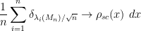
(in the vague topology) where 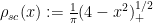 is the semicircular distribution. (See these lecture notes on this blog for more discusssion of this law.)
One can phrase this law in a number of equivalent ways. For instance, in the bulk region  , one almost surely has

uniformly for in  , where the classical location
 ![{\gamma_i \in [-2,2]}](https://s0.wp.com/latex.php?latex=%7B%5Cgamma_i+%5Cin+%5B-2%2C2%5D%7D&bg=ffffff&fg=000000&s=0&c=20201002) of the (normalised)
of the (normalised)  eigenvalue
  is defined by the formula

The bound (1) also holds in the edge case (by using the operator norm bound  , due to Bai and Yin), but for sake of exposition we shall restriction attention here only to the bulk case.
From (1) we see that the semicircular law controls the eigenvalues at the coarse scale of  . There has been a significant amount of work in the literature in obtaining control at finer scales, and in particular at the scale of the average eigenvalue spacing, which is of the order of
  . For instance, we now have a universal limit theorem for the normalised eigenvalue spacing
  in the bulk for all Wigner matrices, a result of Erdos, Ramirez, Schlein, Vu, Yau, and myself. One tool for this is the four moment theorem of Van and myself, which roughly speaking shows that the behaviour of the eigenvalues at the scale
  (and even at the slightly finer scale of
  for some absolute constant
  ) depends only on the first four moments of the matrix entries. There is also a slight variant, the three moment theorem, which asserts that the behaviour of the eigenvalues at the slightly coarser scale of
  depends only on the first three moments of the matrix entries.
It is natural to ask whether these moment conditions are necessary. From the result of Erdos, Ramirez, Schlein, Vu, Yau, and myself, it is known that to control the eigenvalue spacing  at the critical scale , no knowledge of any moments beyond the second (i.e. beyond the mean and variance) are needed. So it is natural to conjecture that the same is true for the eigenvalues themselves.
The main result of this paper is to show that this is not the case; that at the critical scale , the distribution of eigenvalues  is sensitive to the fourth moment, and so the hypothesis of the four moment theorem cannot be relaxed.
Heuristically, the reason for this is easy to explain. One begins with an inspection of the expected fourth moment
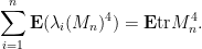
A standard moment method computation shows that the right hand side is equal to
where  is the fourth moment of the real part of the off-diagonal coefficients of . In particular, a change in the fourth moment by
  leads to a change in the expression
  by
by  . Thus, for a typical , one expects
  to shift by
  ; since
  on the average, we thus expect itself to shift by about
  by the mean-value theorem.
To make this rigorous, one needs a sufficiently strong concentration of measure result for that keeps it close to its mean value. There are already a number of such results in the literature. For instance, Guionnet and Zeitouni showed that was sharply concentrated around an interval of size  around
  for any
  (in the sense that the probability that one was outside this interval was exponentially small). In one of my papers with Van, we showed that was also weakly concentrated around an interval of size
  around , in the sense that the probability that one was outside this interval was
  for some absolute constant . Finally, if one made an additional log-Sobolev hypothesis on the entries, it was shown by by Erdos, Yau, and Yin that the average variance of as varied from
  to
to  was of the size of for some absolute .
As it turns out, the first two concentration results are not sufficient to justify the previous heuristic argument. The Erdos-Yau-Yin argument suffices, but requires a log-Sobolev hypothesis. In our paper, we argue differently, using the three moment theorem (together with the theory of the eigenvalues of GUE, which is extremely well developed) to show that the variance of each individual is (without averaging in ). No log-Sobolev hypothesis is required, but instead we need to assume that the third moment of the coefficients vanishes (because we want to use the three moment theorem to compare the Wigner matrix to GUE, and the coefficients of the latter have a vanishing third moment). From this we are able to make the previous arguments rigorous, and show that the mean  is indeed sensitive to the fourth moment of the entries at the critical scale .
One curious feature of the analysis is how differently the median and the mean of the eigenvalue react to the available technology. To control the global behaviour of the eigenvalues (after averaging in ), it is much more convenient to use the mean, and we have very precise control on global averages of these means thanks to the moment method. But to control local behaviour, it is the median which is much better controlled. For instance, we can localise the median of to an interval of size , but can only localise the mean to a much larger interval of size . Ultimately, this is because with our current technology there is a possible exceptional event of probability as large as for which all eigenvalues could deviate as far as from their expected location, instead of their typical deviation of . The reason for this is technical, coming from the fact that the four moment theorem method breaks down when two eigenvalues are very close together (less than  times the average eigenvalue spacing), and so one has to cut out this event, which occurs with a probability of the shape . It may be possible to improve the four moment theorem proof to be less sensitive to eigenvalue near-collisions, in which case the above bounds are likely to improve.


Recent Comments