
Previous set of notes: Notes 3. Next set of notes: 246C Notes 1.
One of the great classical triumphs of complex analysis was in providing the first complete proof (by Hadamard and de la Vallée Poussin in 1896) of arguably the most important theorem in analytic number theory, the prime number theorem:
Theorem 1 (Prime number theorem) Letdenote the number of primes less than a given real number
. Then
(or in asymptotic notation,
as
).
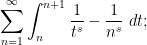
(Actually, it turns out to be slightly more natural to replace the approximation 

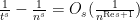
The complex-analytic proof of this theorem hinges on the study of a key meromorphic function related to the prime numbers, the Riemann zeta function 
Definition 2 (Riemann zeta function, preliminary definition) Letbe such that
. Then we define

Note that the series is locally uniformly convergent in the half-plane
The Riemann zeta function has several remarkable properties, some of which we summarise here:
Theorem 3 (Basic properties of the Riemann zeta function)
- (i) (Euler product formula) For any
where the product is absolutely convergent (and locally uniform in
) and is over the prime numbers
.
- (ii) (Trivial zero-free region)
has no zeroes in the region
.
- (iii) (Meromorphic continuation)
and no other poles. Furthermore, the Riemann xi function
is an entire function of order
(after removing all singularities). The function
is an entire function of order one after removing the singularity at
- (iv) (Functional equation) After applying the meromorphic continuation from (iii), we have
for all
for all


Proof: We just prove (i) and (ii) for now, leaving (iii) and (iv) for later sections.
The claim (i) is an encoding of the fundamental theorem of arithmetic, which asserts that every natural number 


 ,
,  , and
, and  consists of all the natural numbers of the form
  for some
  . Sending
  and to infinity, we conclude from monotone convergence and the geometric series formula that
 is real, and then from dominated convergence we see that the same formula holds for complex with as well. Local uniform convergence then follows from the product form of the Weierstrass
  -test (Exercise 19 of Notes 1).
The claim (ii) is immediate from (i) since the Euler product 

We remark that by sending
 . This can be viewed as a weak version of the prime number theorem, and already illustrates the potential applicability of the Riemann zeta function to control the distribution of the prime numbers.
The meromorphic continuation (iii) of the zeta function is initially surprising, but can be interpreted either as a manifestation of the extremely regular spacing of the natural numbers 
Henceforth we work with the meromorphic continuation of 


From Theorem 3 and the non-vanishing nature of 


 by (1), hence for all (except the pole at ) by meromorphic continuation. Thus if is a non-trivial zero then so is
  . We conclude that the set of non-trivial zeroes is symmetric by reflection by both the real axis and the critical line
  . We have the following infamous conjecture:
Conjecture 4 (Riemann hypothesis) All the non-trivial zeroes of
This conjecture would have many implications in analytic number theory, particularly with regard to the distribution of the primes. Of course, it is far from proven at present, but the partial results we have towards this conjecture are still sufficient to establish results such as the prime number theorem.
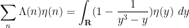
Return now to the original region where


 , where the von Mangoldt function
  is defined to equal
  whenever
  is a power
  of a prime
  for some
  , and
, and  otherwise. The contribution of the higher prime powers
  is negligible in practice, and as a first approximation one can think of the von Mangoldt function as the indicator function of the primes, weighted by the logarithm function.
The series 

Exercise 5 (Standard Dirichlet series) Let
- (i) Show that
.
- (ii) Show that
, where
is the divisor function of
- (iii) Show that
, where
is the Möbius function, defined to equal
when
distinct primes for some
, and
otherwise.
- (iv) Show that
, where
is the Liouville function, defined to equal
- (v) Show that
, where
is the holomorphic branch of the logarithm that is real for
vanishes for
.
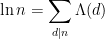
- (vi) Use the fundamental theorem of arithmetic to show that the von Mangoldt function is the unique function
such that
for every positive integer
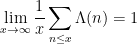
Given the appearance of the von Mangoldt function 
Theorem 6 (Prime number theorem, von Mangoldt form) One has(or in asymptotic notation,
as
Let us see how Theorem 6 implies Theorem 1. Firstly, for any 
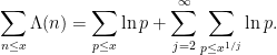
 is non-zero for only
  values of
  , and is of size
  , thus
 , we conclude from Theorem 6 that
  . Next, observe from the fundamental theorem of calculus that
 and summing over all primes
  , we conclude that
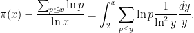
 , thus
 and
and  we see that the right-hand side is
  , and Theorem 1 follows.
Exercise 7 Show that Theorem 1 conversely implies Theorem 6.
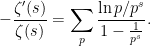
The alternate form (8) of the Euler product identity connects the primes (represented here via proxy by the von Mangoldt function) with the logarithmic derivative of the zeta function, and can be used as a starting point for describing further relationships between
Theorem 8 (Riemann-von Mangoldt explicit formula) For any non-integer, we have
where
. Furthermore, the convergence of the limit is locally uniform in

Actually, it turns out that this formula is in some sense too precise; in applications it is often more convenient to work with smoothed variants of this formula in which the sum on the left-hand side is smoothed out, but the contribution of zeroes with large imaginary part is damped; see Exercise 22. Nevertheless, this formula clearly illustrates how the non-trivial zeroes

 )
) 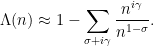
 induces an oscillation in the von Mangoldt function, with
  controlling the frequency of the oscillation and
  the rate to which the oscillation dies out as
  . This relationship is sometimes known informally as “the music of the primes”.
Comparing Theorem 8 with Theorem 6, it is natural to suspect that the key step in the proof of the latter is to establish the following slight but important extension of Theorem 3(ii), which can be viewed as a very small step towards the Riemann hypothesis:
Theorem 9 (Slight enlargement of zero-free region) There are no zeroes of.
It is not quite immediate to see how Theorem 6 follows from Theorem 8 and Theorem 9, but we will demonstrate it below the fold.
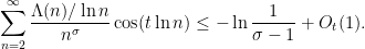
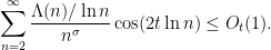
Although Theorem 9 only seems like a slight improvement of Theorem 3(ii), proving it is surprisingly non-trivial. The basic idea is the following: if there was a zero at 


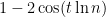 can be negative for large regions of the variable , whereas is always non-negative. This conflict eventually leads to a contradiction, but it is not immediately obvious how to make this argument rigorous. We will present here the classical approach to doing so using a trigonometric identity of Mertens.
In fact, Theorem 9 is basically equivalent to the prime number theorem:
Exercise 10 For the purposes of this exercise, assume Theorem 6, but do not assume Theorem 9. For any non-zero realas
, where
denotes a quantity that goes to zero as
. Use this to derive Theorem 9.

This equivalence can help explain why the prime number theorem is remarkably non-trivial to prove, and why the Riemann zeta function has to be either explicitly or implicitly involved in the proof.
This post is only intended as the briefest of introduction to complex-analytic methods in analytic number theory; also, we have not chosen the shortest route to the prime number theorem, electing instead to travel in directions that particularly showcase the complex-analytic results introduced in this course. For some further discussion see this previous set of lecture notes, particularly Notes 2 and Supplement 3 (with much of the material in this post drawn from the latter).
— 1. Meromorphic continuation and functional equation —
We now focus on understanding the meromorphic continuation of 

One way to motivate the meromorphic continuation


 , it is a routine application of the Fubini and Morera theorems to establish analytic continuation of the residual to the half-plane
  , thus giving a meromorphic extension
  to the region
  . Among other things, this shows that (the meromorphic continuation of) has a simple pole at with residue .
Exercise 11 Using the trapezoid rule, show that for anywith
, there exists a unique complex number
for any natural number
, where
. Use this to extend the Riemann zeta function meromorphically to the region
and
.

Exercise 12 Obtain the refinement
to the trapezoid rule when
are integers and
is continuously three times differentiable. Then show that for any
with
for any natural number
.


One can keep going in this fashion using the Euler-Maclaurin formula (see this previous blog post) to extend the range of meromorphic continuation to the rest of the complex plane. However, we will now proceed in a different fashion, using the theta function

 of the argument in the upper half-plane (so
  ); from Exercise 7 of Notes 2 we have the modularity relation
 decays exponentially to as , blows up like
  as
as  .
.
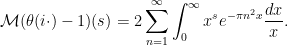
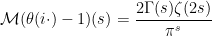
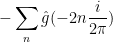
We will attempt to apply the Mellin transform (Exercise 11 from Notes 2) to this function; formally, we have
 := \int_0^\infty x^s \theta(ix) \frac{dx}{x}.](https://s0.wp.com/latex.php?latex=%5Cdisplaystyle++%7B%5Cmathcal+M%7D%5B%5Ctheta%28i%5Ccdot%29%5D%28s%29+%3A%3D+%5Cint_0%5E%5Cinfty+x%5Es+%5Ctheta%28ix%29+%5Cfrac%7Bdx%7D%7Bx%7D.&bg=ffffff&fg=000000&s=0&c=20201002) goes to infinity, converges to one, and the integral here is unlikely to be convergent. So we will compute the Mellin transform of
goes to infinity, converges to one, and the integral here is unlikely to be convergent. So we will compute the Mellin transform of  :
: 
 decays exponentially as , and blows up like
  as , so this integral will be absolutely integrable when
  . Since


 . Replacing by
  , we can rearrange this as a formula for the
  function (4), namely
  .
.
Now we exploit the modular identity (12) to improve the convergence of this formula. The convergence of 


 to obtain


 . However, the integrand here is holomorphic in and exponentially decaying in , so from the Fubini and Morera theorems we easily see that the right-hand side is an entire function of ; also from inspection we see that it is symmetric with respect to the symmetry
  . Thus we can define as an entire function, and hence as a meromorphic function, and one verifies the functional equation (6).
It remains to establish that 


 (say), and hence is of order at most as required. (One can show that has order exactly one by inspecting what happens to
  as
as  , using that
  in this regime.) This completes the proof of Theorem 3.
Exercise 13 (Alternate derivation of meromorphic continuation and functional equation)
- (i) Establish the identity
whenever
- (ii) Establish the identity
whenever
,
where
is the branch of the logarithm with imaginary part in
, and
is the contour consisting of the line segment
, the semicircle
, and the line segment
.
- (iii) Use (ii) to meromorphically continue
.
- (iv) By shifting the contour
for a large natural number
again using the branch
.
- (v) Establish the functional equation (5).


Exercise 14 Use the formulafrom Exercise 12, together with the functional equation, to give yet another proof of the identity
.
Exercise 15 (Relation between zeta function and Bernoulli numbers)
- (i) For any complex number
with
, use the Poisson summation formula (Proposition 3(v) from Notes 2) to establish the identity
- (ii) For
Conclude that
for any natural number
are defined through the Taylor expansion
Thus for instance
,
, and so forth.
- (iii) Show that
for any odd natural number
- (iv) Use (14) and the residue theorem (now working inside the contour
, rather than outside) to give an alternate proof of (15).


Exercise 16 (Convexity bounds)It is possible to improve the bounds (iii) in the region
- (i) Establish the bounds
for any
and
with
.
- (ii) Establish the bounds
for any
and
- (iii) Establish the bounds
for any
and
; such improvements are known as subconvexity estimates. For instance, it is currently known that
for any
and
, although this remains unproven (it is however a consequence of the Riemann hypothesis).
Exercise 17 (Riemann-von Mangoldt formula) Show that for any, the number of zeroes of
is equal to
. (Hint: apply the argument principle to
for some
that is chosen so that the horizontal edges of the rectangle do not come too close to any of the zeroes (cf. the selection of the radii
in the proof of the Hadamard factorisation theorem in Notes 1), and use the functional equation and Stirling’s formula to control the asymptotics for the horizontal edges.)
We remark that the error term
, due to von Mangoldt in 1905, has not been significantly improved despite over a century of effort. Even assuming the Riemann hypothesis, the error has only been reduced very slightly to
(a result of Littlewood from 1924).
Remark 18 Thanks to the functional equation and Rouche’s theorem, it is possible to numerically verify the Riemann hypothesis in any finite portionof the critical strip, so long as the zeroes in that strip are all simple. Indeed, if there was a zero
off of the critical line
, then an application of the argument principle (and Rouche’s theorem) in some small contour around
on the critical line, applying the argument principle for some small contour around that zero and symmetric around the critical line would numerically verify that there was exactly one zero within that contour, which by the functional equation would then have to lie exactly on that line. (In practice, more efficient methods are used to numerically verify the Riemann hypothesis over large finite portions of the strip, but we will not detail them here.)
— 2. The explicit formula —
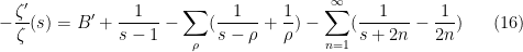
We now prove Riemann-von Mangoldt explicit formula. Since
 , where ranges over the non-trivial zeroes of (note from Exercise 11 that there is no zero at the origin), and
  is some constant. From (4) we can calculate
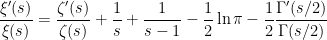
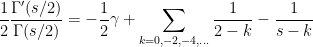
One can compute the values of 
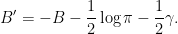
Exercise 19 By inspecting both sides of (16) as, show that
, and hence
.
Jensen’s formula tells us that the number of non-trivial zeroes of 


Exercise 20 (Local bound on zeroes)
- (i) Establish the upper bound
whenever
and
. (Hint: use (10). More precise bounds are available with more effort, but will not be needed here.)
- (ii) Establish the bounds
uniformly in
- (iii) Show that for any
is
- (iv) For
, and
, with
(Hint: use Theorem 9 of Notes 1.)

Meanwhile, from Perron’s formula (Exercise 12 of Notes 2) and (8) we see that for any non-integer 
Exercise 21 (Riemann-von Mangoldt explicit formula) Let(Hint: for (i)-(iii), shift the contour
- (i)
.
- (ii)
.
- (iii) For any positive integer
- (iv) For any non-trivial zero
- (v) We have
.
- (vi) We have
.
to
for an
that gets sent to infinity, and using the residue theorem. The same argument works for (iv) except when
, in which case a detour to the contour may be called for. For (vi), use Exercise 20 and partition the zeroes depending on what unit interval
falls into.)
- (viii) Using the above estimates, conclude Theorem 8.


The explicit formula in Theorem 8 is completely exact, but turns out to be a little bit inconvenient for applications because it involves all the zeroes
Exercise 22 (Smoothed explicit formula)
- (i) Let
be a smooth function compactly supported on
. Show that
is entire and obeys the bound
(say) for some
, all
, and all
- (ii) With
as in (i), establish the identity
with the summations being absolutely convergent by applying the Fourier inversion formula to
for some
, applying (8), and then shifting the contour again (using Exercise 20 and (i) to justify the contour shifting).
- (iii) Show that
whenever
is a smooth function, compactly supported in
, with the summation being absolutely convergent.
- (iv) Explain why (iii) is formally consistent with Theorem 8 when applied to the non-smooth function
.


— 3. Extending the zero free region, and the prime number theorem —
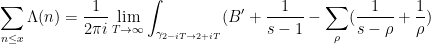
We now show how Theorem 9 implies Theorem 6. Let 

![{[2,x]}](https://s0.wp.com/latex.php?latex=%7B%5B2%2Cx%5D%7D&bg=ffffff&fg=000000&s=0&c=20201002)
![{[1.5, x + x/T]}](https://s0.wp.com/latex.php?latex=%7B%5B1.5%2C+x+%2B+x%2FT%5D%7D&bg=ffffff&fg=000000&s=0&c=20201002)

![{y \in [1.5,2]}](https://s0.wp.com/latex.php?latex=%7By+%5Cin+%5B1.5%2C2%5D%7D&bg=ffffff&fg=000000&s=0&c=20201002) and
and  , and
, and 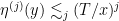
![{y \in [x,x+T]}](https://s0.wp.com/latex.php?latex=%7By+%5Cin+%5Bx%2Cx%2BT%5D%7D&bg=ffffff&fg=000000&s=0&c=20201002) and . Such a function can be constructed by gluing together various rescaled versions of (antiderivatives of) standard bump functions. For such a function, we have
and . Such a function can be constructed by gluing together various rescaled versions of (antiderivatives of) standard bump functions. For such a function, we have 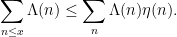


 and
and  , where
  is a parameter to be chosen later. For , there are only
  zeros, and all of them have real part strictly less than by Theorem 9. Hence there exists
  such that
  for all such zeroes. For each such zero, we have from the triangle inequality
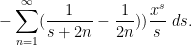
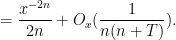
 . For each zero with
  , we integrate parts twice to get some decay in :

 we conclude
 is convergent (this follows from Exercise 20 we conclude (for
  large enough depending on
  ) that the total contribution here is
  . Thus, after choosing suitably, we obtain the bound
 is sufficiently large depending on (since
  depends only on , which depends only on ). A similar argument (replacing
  by
by  in the construction of
  ) gives the matching lower bound
  is sufficiently large depending on . Sending
  , we obtain Theorem 6.
Exercise 23 Assuming the Riemann hypothesis, show thatfor any
for any
to the region
was first holomorphically continued to the region
).


It remains to prove Theorem 9. The claim is clear for 

 sufficiently close to . Taking logarithms, we see in particular that
 that gives
  sufficiently close to one, and on taking logarithms as before we get
 close to
  for most numbers that are weighted by
  . To get the contradiction, we use the analytic continuation of to
  to conclude that

 is close to then
  has to be close to
  ) as well as the non-negative nature of to conclude that
 , and proves the prime number theorem.
Exercise 24 Establish the inequalityfor any

Remark 25 There are a number of ways to improve Theorem 9 that move a little closer in the direction of the Riemann hypothesis. Firstly, there are a number of zero-free regions for the Riemann zeta function known that give lower bounds for(and in particular preclude the existence of zeros) a small amount inside the critical strip, and can be used to improve the error term in the prime number theorem; for instance, the classical zero-free region shows that there are no zeroes in the region
for some sufficiently small absolute constant
, and lets one improve the
error term in Theorem 6 to
(with a corresponding improvement in Theorem 1, provided that one replaces
with the logarithmic integral

81 comments
Comments feed for this article
12 February, 2021 at 9:53 am
pcaceres00
I would appreciate if someone could comment on the attached paper. Fascinating subject.
Many thanks in advance
Pedro Caceres
(763) 412-8915
12 February, 2021 at 9:56 am
pcaceres00
It would help if I add the link!
https://www.researchgate.net/publication/340296254_An_Engineer's_Approach_to_the_Riemann_Hypothesis_and_why_it_is_true
12 February, 2021 at 10:16 am
Raphael
“In this paper we will provide a proof of the RH.” Possibly one or more such papers are published every day. Here to see quickly if possibly could make sense to have a look on one of them https://www.scottaaronson.com/blog/?p=304 .
12 February, 2021 at 11:12 am
Anonymous
In the second line, “la” is missing from the name de la Vallee Poussin
12 February, 2021 at 11:16 am
Anonymous
In (2), 645 should be 945
12 February, 2021 at 12:21 pm
Anonymous
In theorem 3, it may be added that Euler product (3) is locally uniformly convergent (which may be used later to justify the term-wise logaritmic derivative to obtain (8) – without using Fubini theorem)
12 February, 2021 at 12:47 pm
Rex
“…from the divergence of the harmonic series we then conclude Euler’s theorem . This can be viewed as a weak version of the prime number theorem,…”
I believe I heard somewhere the heuristic that a subset of the natural numbers has divergent reciprocal sum if and only if, roughly speaking, its density declines at rate or slower. Is this true?
[Yes; this follows fairly readily from the Cauchy condensation test. For instance, density decaying faster than will ensure convergence, whereas density that stays above
  for all sufficiently large
  will guarantee divergence. -T]
12 February, 2021 at 12:59 pm
Rex
So then the divergence of prime reciprocals already gives us yet another simple proof of “the prime number theorem up to a constant”?
[Not quite; the density could be wildly fluctuating to be significantly denser than at some scales and significantly sparser at other scales. -T]
12 February, 2021 at 6:39 pm
Lior Silberman
Not quite: the Cauchy condensation test applies to monotone series, and here you don’t know that the density of primes is monotone. Maybe there are long stretches with no primes (so the density falls low), follows by long sequences with many primes (so the density becomes large).
12 February, 2021 at 1:03 pm
Rex
“We remark that by sending to
to  in Theorem 3(i) we conclude that
It seems here we are implicitly using some Tauberian theorem or other, to assert that the divergence of as
as  implies the divergence of the partial sums of
  ? And similarly on the product side?
[Monotone convergence suffices here. -T]
12 February, 2021 at 3:24 pm
Theorist
I think, contrary to the prime number theorem, the equivalent relation that p_n is asymptotic to n ln(n), where p_n is the n-th prime itself, is much less known. By the way, this relation in turn is equivalent to the nice result that the p_n-th root of n^n tends to Euler’s number e if n tends to infinity.
12 February, 2021 at 6:34 pm
Anonymous
I have been looking for the original proof of the prime number theorem. Thank you!
12 February, 2021 at 6:43 pm
Lior Silberman
The original proof is due to Riemann (1859) (conditioned on the Riemann hypothesis). The essential ideas are there except for the proof that there are no zeroes on the line , and for the more delicate handling this required compared with the case where the zeroes are well off that line.
12 February, 2021 at 8:31 pm
Aditya Guha Roy
Lior I doubt that. I think the first proof was given by Hadamard and Poussin independently around the same time. Their proofs were heavily based on analysing a result due to Chebyshev on Chebyshev functions, and both used complex analytic methods quite heavily.
Once this proof was found, people wanted to somehow eliminate the complex analytic ingredients in quest to obtain an “elementary” proof of the result. There are also reports of several debates among mathematicians during that time on whether any such non complex analytic proof can be found or not. It is also believed that Hardy carried the impression that the prime number theorem draws so heavily on analysis of the zeta function, that eliminating the complex analytic ingredients from any proof of the result is almost impossible.
Much later the first and also the only such “elementary” proof was found independently by Paul Erdos and Atle Selberg, both using an identity due to Selberg.
Even later a very short proof was found by Newman. It is perhaps the shortest known proof of the prime number theorem and uses only very basic level complex analysis, such as those of analytic continuation and evaluation of contour integrals.
Towards the end of 2020 I read a nice article on the timeline of the prime number theorem, with some reports on debates among mathematicians on non-complex analytic proofs of the result, as well as the issue of rewarding the Fields Medal to Atle Selberg and not Erdos for the elementary proof, but I cannot find it unfortunately (:( ). If someone find it or if I find it, do comment below.
13 February, 2021 at 12:23 am
Ulrich
This one:
Click to access erdosselberg.pdf
13 February, 2021 at 6:02 am
Anonymous
Both Selberg and Erdos contributed to the proof (Selberg initially thought that his important estimate was not sufficient to prove the PNT, but Erdos showed him how to prove the PNT from Selberg’s estimate)
Unfortunately, Selberg chose to publish a separate proof (based on another derivation of the PNT from his basic estimate) – thereby forcing Erdos to publish separately his original derivation of the PNT from Selberg’s basic estimate.
13 February, 2021 at 9:47 am
Lior Silberman
Aditya: as I explained above, Riemann indeed proved the Prime Number Theorem, conditionally on the Riemann Hypothesis. Conditional proofs have a long history in mathematics — most famously Serre and Ribet proving Fermat’s Last Theorem conditionally on the Tanyiama–Shimura Conjecture, which was later substantially proved by Wiles.
Riemann’s memoir contains most of the key ideas of the proof. De la Valée Poussin and Hadamard completed the work by giving the first unconditional proofs, but Riemann’s contribution is still the greater.
Mathematics is a race where often winners are declared by coming last: whoever makes the final contribution gets the glory. Sometimes it’s right (the hardest part is often left for last, after all), but sometimes it’s wrong: until the earlier work there was no room for the later. Before Riemann there was no avenue to prove the PNT at all. After Riemann there was a conditional proof and a clear direction.
For the same reason I credit FLT to Ribet, and the Modularity Theorem to Wiles. Here Wiles’s contribution is greater (the proof of the FLT is mainly of historical importance, while modularity is an essential part of mathematics), but still the FLT was proved by Ribet, not Wiles.
13 February, 2021 at 11:51 pm
Aditya Guha Roy
Ah, I see your point of view, Lior. If you like to call / view it that way then it’s fair enough.
By “original” I meant the first complete proof which doesn’t assume anything which is not known till date.
By the way just some nitpicking : given that the truth of Riemann hypothesis is not known till date, would you still say that Riemann “proved” the prime number theorem?
(Of course now that we know the PNT is true so ex falso quodlibet plays the game.)
13 February, 2021 at 9:58 am
Rex
I’ve wondered whether Riemann was the very first person to introduce complex methods into number theory. Do you know if Dirichlet’s proof of arithmetic progressions used it in any essential way?
13 February, 2021 at 7:18 pm
Lior Silberman
Indeed Riemann completely revolutionized the field, which is why I credit him with a proof of the PNT. He both had a rigorous conditional proof (subject to RH) and charted the path for the first unconditional proofs.
Dirichlet’s proof of his theorem is based on Euler’s proof of the infinitude of primes (discussed above after Theorem 3), and lives entirely on the real axis. He originally only used the pole to show that there were infinitely many primes in each admissible arithmetic progression, and later observed that the proof is actually quantitative: generalizing Mertens’s Theorem
Dirichlet shows (purely by real-variable methods, even if some later proofs use complex methods)
13 February, 2021 at 11:55 pm
Aditya Guha Roy
Rex, if you go through Dirichlet’s proof of Dirichlet’s theorem, you will find that his proof did involve complex analytic ingredients in it in analysing the L functions which were crucially used in proving the result.
14 February, 2021 at 11:35 am
Lior Silberman
Aditya: Dirichlet’s proof (I link to an English translation) did not use complex analysis at all. Today (with the benefit of hindsight) we can see that his arguments prove that his L-series have analytical continuation to the half-plane . But if you read the paper carefully you’ll see that the parameter
  only takes real values. The values
  are complex (because the Dirichlet characters take complex values), but that does not make the proof involve complex analysis. In fact Dirichlet is careful to argue about real and complex parts separately.
The paper is interesting also for Dirichlet’s calling attention to the distinction between absolutely convergent and conditionally convergent series, and showing he was aware that conditionally convergent series could be rearranged to sum to different values (what we call today “Riemann’s Rearrangement Theorem”).
14 February, 2021 at 11:36 am
Lior Silberman
Here’s the link to the proof since it didn’t work in the comment above (a double quotes symbol is off in the HTML)
https://arxiv.org/abs/0808.1408
14 February, 2021 at 8:30 pm
Aditya Guha Roy
Ah, thanks Lior. I didn’t know of this. I read the proof from Davenport’s text on MNT, and I developed the impression that the proof discussed in the text is what Dirichlet actually did himself. Thank you for the link.
13 February, 2021 at 3:33 am
Aditya Guha Roy
Reblogged this on Aditya Guha Roy's weblog.
13 February, 2021 at 6:25 am
Rex
“By splitting the integral into the ranges and
and  we see that the right-hand side is
  , and Theorem 1 follows."
I've seen this strategy of decomposing an integral or sum into ranges above and below in several places, to bound the pieces separately. But I've never really understood the basic principle behind why it works. Why is
  a good cutoff to use?
14 February, 2021 at 10:24 am
Terence Tao
The most difficult term to understand in the integral is the term, which varies in
  . But within the range
 ![y \in [\sqrt{x},x]](https://s0.wp.com/latex.php?latex=y+%5Cin+%5B%5Csqrt%7Bx%7D%2Cx%5D&bg=ffffff&fg=545454&s=0&c=20201002) ,
,  is constant (up to bounded multiplicative error), so this term can be simplified. In general, when trying to estimate an integral, it can often be beneficial to break up into pieces where one or more of the terms in the integral is approximately constant, as one can then often replace that term by the constant and get an easier expression to estimate which is still equivalent to the original expression up to constants. One could have replaced
  here by other small powers of
  , but this is as good a choice as any here as the contribution of the very small
  ends up being negligible and can be controlled satisfactorily by virtually any estimate.
13 February, 2021 at 8:38 am
Rex
“From (6) we certainly have , thus
 ”
”
It seems the reference (6) wants to refer to the (unnumbered) formula five lines up, but it’s not actually directing to this.
[Corrected, thanks – T.]
14 February, 2021 at 1:27 pm
Rex
“or (writing )
)
 ”
”
I think here you want the bottom exponent to be ?
?
[Corrected, thanks – T.]
14 February, 2021 at 2:44 pm
Avi Levy
Just as the “ as Mellin transform of
  ” point of view explains how the Poisson summation formula is the source of the critical line reflection symmetry, it brings up a (vague and ill-posed) question about the nature of the square root fluctuations in the explicit formula.
 is a fixed point of this symmetry. On the other hand, there are “randomness of the primes” heuristics where the
  comes from Brownian fluctuations, which traces its source to linearity of variance for sums of independent random variables.
On the one hand, the exponent
Are these two explanations of the square root fluctuations somehow connected? Or is it akin to phenomena in statistical physics models where the self-dual point happens to coincide with the critical point, as in https://arxiv.org/abs/1006.5073 for example?
14 February, 2021 at 3:03 pm
Anonymous
It is related to the idea of “square root cancellation”
18 February, 2021 at 3:20 pm
Terence Tao
Hmm, interesting question. Certainly probabilistic methods can be used without any appeal to the functional equation to give some statistical control on say the Riemann zeta function in the region , for instance one can show without much difficulty (basically the
  mean value theorem) that almost all of the zeroes avoid the region
  for any fixed
  . Here the “1/2” is the same 1/2 that comes from Brownian motion, or more generally in applications of the second moment method. This is only consistent with a functional equation if the critical line of that functional equation is at or to the left of
  . On the other hand I don’t see a probabilistic argument that explains why the critical line has to be exactly at
  ; this would involve some way to understand zeta to the left of the critical line that does not involve the functional equation. Still, this sort of coincidence between the abscissa coming from second moment considerations and the abscissa coming from the functional equation does seem to be pretty universal amongst all the other L-functions in number theory so presumably there is a more robust explanation of this phenomenon.
14 February, 2021 at 2:55 pm
Anonymous
In the Wikipedia article on the zeta function it is remarked that the functional equation (5) was discovered and conjectured by Euler (for integer values of ) in 1749.
15 February, 2021 at 12:45 am
justderiving
What would happen to the field of math if the Riemann hypothesis were proven false or true?
19 December, 2021 at 4:52 am
Aditya Guha Roy
If the Riemann hypothesis turns out to be true then it would be more exciting than any other discovery in number theory in the last few decades. It will also answer several other questions in different parts of mathematics, and also outside mathematics.
Of course, if it can be proved that RH is false, that would also be an amazing discovery, but probably that will not make us that happy, as the hope for many other things will be lost.
There are several papers (which are authentic and reviewed) on several equivalences of RH on the internet.
15 February, 2021 at 12:59 pm
Rex
“from Exercise 11 that there is no zero at the origin), and is some constant. From (4) we can calculate
 ”
”
This formula is missing on the right.
[Corrected, thanks – T.]
18 February, 2021 at 4:13 pm
Rex
Is it just me, or is it still missing?
[Corrected, thanks – T.]
23 February, 2021 at 5:34 am
Rex
Also, there is now an extraneous in the formula immediately above this one. Probably from the first attempt to fix it.
[Corrected, thanks – T.]
15 February, 2021 at 9:15 pm
Joseph Sugar
Riemann states in his paper that he is interested in the prime numbers’ density distribution, not in finding more precise prime number theorems. His formula for x = 2000.000 is exact, so finding better and better approximations was probably already not very exciting.
15 February, 2021 at 11:41 pm
anthonyquas
In the proof of Theorem 3(i), you have used monotone convergence, but that’s only good for $s$ real and positive, right?
16 February, 2021 at 3:03 pm
Lior Silberman
Yes. The proof above uses monotone convergence for real and positive (actually for
  ), and then dominated convergence to go from there to the halfplane
  .
.
17 February, 2021 at 10:50 am
Anonymous
I believe in Exercise 12, it should be rather than
  ? (The current version seems to give
  ).
).
[Corrected, thanks – T.]
18 February, 2021 at 8:57 am
Aditya Guha Roy
Thought this would be relevant: https://mathoverflow.net/questions/58004/how-does-one-motivate-the-analytic-continuation-of-the-riemann-zeta-function/380502#380502 here prof. Tao discusses a nice way to motivate (/ see naturally) the meromorphic continuation of the zeta function.
18 February, 2021 at 2:21 pm
Anonymous
I believe the exponent in equation (12) should be +1/2, not -1/2. Thank you for posting these great notes!
[Corrected, thanks – T.]
19 February, 2021 at 6:21 am
Anonymous
Dear respected Pro.Tao,
Is there any relationship between you and my night dream?
In 2019, I dreamed about numbers but not clear. A month later, you claimed that you proved Collatz conjecture. In 2020, I also dreamed about many numbers but not clear. Strangely, a month later, you announced that you proved Sendov conjecture. But this time, with the third night dream one month ago in 2021, I had seen many numbers, many equations x, y,z , many maths signals very long and densly . I saw them very clearly like at noon, different from two previous dreams. I am happy myself and I wonder whether Pro.Tao is going to claim proving one clay millenium problem successfully. I hope my third dream is right certainly. My guess that they are Riemann hypothesis, Navier Stokes existence and smoothness, Birch Swinerton Dyer conjecture.
Bye Pro Tao.( I always wait good news from you)
27 February, 2021 at 9:14 am
Course announcement: 246B, complex analysis | What's new
[…] (if time permits) the Riemann zeta function and the prime number theorem. […]
27 February, 2021 at 9:38 am
246B, Notes 3: Elliptic functions and modular forms | What's new
[…] Previous set of notes: Notes 2. Next set of notes: Notes 4. […]
27 February, 2021 at 9:47 am
246C notes 1: Meromorphic functions on Riemann surfaces, and the Riemann-Roch theorem | What's new
[…] set of notes: 246B Notes 4. Next set of notes: Notes 2. The fundamental object of study in real differential geometry are the […]
27 February, 2021 at 9:12 pm
Frank Vega
Good notions (Thanks…)!!! It’s great to obtain for free just already summarized many things here (into a single page instead of trying to find them from many reference papers). I didn’t see the Lagarias and Robin inequalities here. Maybe, they are in the previous posts related to this one. Proving the RH by proving a simple inequality looks very attractive. However, behind these inequalities, we could find a deep estimates on the distribution of primes. I have moved forward in this tempting direction:
https://doi.org/10.5281/zenodo.3648511
What do you think?
9 March, 2021 at 6:15 am
An elementary proof of divergence of the sum of reciprocal of prime numbers | Aditya Guha Roy's weblog
[…] of primes diverges by contrasting it with the already-known-to-be-divergent harmonic sum (see this blogpost by professor Terence Tao for more details); in this blogpost I discuss a proof of the […]
12 March, 2021 at 6:27 am
Aditya Guha Roy
In case anyone is interested (like I was) https://www.claymath.org/publications/riemanns-1859-manuscript
here you can find the versions (such as the original paper, its German transcription, English translation etc.) of Riemann’s paper where he analyzed the zeta function, introduced the xi function etc..
Fact:
This is the only paper Riemann wrote on number theory, and as we all know today this changed the way we look at several topics in number theory and in a sense contributed the most towards development of the modern day subject of analytic number theory.
Also see some comments above by Dr. Lior for further discussion on his methods and related things.
19 March, 2021 at 8:49 am
Guillaume
Dear Terence,
You write that “the Riemann zeta function has to be either explicitly or implicitly involved in [any] proof [of the PNT]”. Could you explain if this applies (and how) to Florian Richter’s recent new elementary proof as well? (arXiv:2002.03255)
(I mean, is there a way to re-understand Richter’s proof, or in a way to see where it comes from or rediscover it, in terms the zeta function?)
20 March, 2021 at 12:45 am
Aditya Guha Roy
Hi Guillaume, let me say what I think is relevant.
It is true that there can exist proofs which do not involve analysing the Riemann zeta function “explicitly”, for instance Erdos and Selberg (to some extent independently) gave an elementary proof of the PNT which actually doesn’t call for any explicit analysis of the Riemann zeta function. in the upper half plane
  involving prime numbers; this connection is the reason why the conclusion of the PNT and the behaviour of the zeta function are so implicitly related.
However the Riemann zeta function is always connected to the ingredients of the prime number theorem and hence with the PNT as well, thanks to the fundamental theorem of arithmetic (and as a consequence the Euler’s product formula) which allows us to write the zeta function evaluated at some point
Thus to put it in a nutshell, the connection of the prime numbers and the zeta function is really very fundamental to understanding the behaviour of the primes and hence any result such as the prime number theorem is believed to have some implicit or explicit connection with the zeta function.
For a broader discussion on how Riemann came about this connection you can read his paper which is mentioned in the blogpost above or in one of the above comments by me.
28 March, 2021 at 2:53 pm
Terence Tao
From Fourier or complex-analytic methods, the prime number theorem is equivalent to the non-vanishing on the right edge of the critical strip. From a pretentious number theory viewpoint, this non-vanishing amounts to the M\”obius function
  “pretending” to be like the function
  , in the sense that
  for almost all large primes. So the hard part of any proof of the PNT (elementary or otherwise) comes about in eliminating the
  scenario. In this perspective, the classical complex analytic proof proceeds basically by observing that
  would imply
  which would eventually lead to a pole forming at
  . The elementary proof of Erdos and Selberg basically exploits the Brun-Titchmarsh inequality to show that the large primes cannot all concentrate in the region
  .
.
Viewing Richter’s proof (or the similar recent elementary proof by McNamara) in this lens, the point is that a weak version of Brun-Titchmarsh (that can be proven by the classical methods of Chebyshev) is again enough to preclude the large primes concentrating in a region such as , though the nice thing about these proofs is that the frequency parameter
  does not make an explicit appearance, and is instead only implicit through the application of iterated multiplicative convolution (Richter studies products of
  primes for some large
  , while McNamara instead compares the distribution of primes with the distribution of semiprimes.) (The Erdos-Selberg proof similarly hides the role of the frequency parameter
  , traditionally through the use of various Tauberian theorems.)
3 April, 2021 at 7:00 am
Riemann zeta function from an elementary level number theoretic viewpoint: a prelude to the Riemann zeta function | Aditya Guha Roy's weblog
[…] an earlier blogpost I re-blogged a very interesting blogpost on the Riemann zeta function, the prime number theorem and their connections with complex analysis […]
25 April, 2021 at 9:19 pm
Riemann zeta function: connections with the von Mangoldt function and a look at the prime number theorem | Aditya Guha Roy's weblog
[…] a particular emphasis on relating it to the von-Mangoldt function. The contents here are based on this blogpost on the topic by professor Terence […]
4 May, 2021 at 5:28 pm
project_2501
I am a beginner in this field. I am intrigued by the statement:
“”
We remark that by sending {s} to 1 in Theorem 3(i) we conclude that
\displaystyle \sum_{n=1}^\infty \frac{1}{n} = \prod_p (1-\frac{1}{p})^{-1}
and from the divergence of the harmonic series we then conclude Euler’s theorem {\sum_p \frac{1}{p} = \infty}
“”
I have only seen more laborious proofs that the sum of prime reciprocals diverges. This suggests the proof is immediate from the Euler product formula.
Can someone explain to me how?
The closest I have found is this, but experts told me that the proof is wrong:
https://math.stackexchange.com/questions/4114982/validity-of-taking-log-of-divergent-sums-in-proof-sum-1-p-rightarrow-infty
18 December, 2021 at 7:03 am
Aditya Guha Roy
Technically speaking, the proof in the link is incomplete because although we have the convergence of each of the partial sums for
for  there are infinitely many of them.
However, we don’t need to do all this.
Just expand the terms in terms of geometric sums and then use the distributive property and divergence of the harmonic series to establish the claim.
18 December, 2021 at 7:12 am
Aditya Guha Roy
If you want to send to get the claim, then you can use the monotone convergence theorem.
22 July, 2021 at 4:12 am
Riemann zeta function: standard Dirichlet series associated with the Riemann zeta function | Aditya Guha Roy's weblog
[…] Dirichlet series associated with the Riemann zeta function and is relevant to Exercise 5 from this blogpost by professor Terence […]
17 December, 2021 at 9:40 am
liki mitica
Dear Professor Tao,
I am one of enthusiasts of your blog, a great place to read and learn about the (new) trends in math. I found 2 days ago an interesting preprint (researchsquare.com) that approaches the Riemann Hypothesis from a different prospective:
DOI: https://doi.org/10.21203/rs.3.rs-1159792/v1
From the abstract: ‘As an application we proved the injectivity of the integral operator involved in the equivalent formulations of Riemann Hypothesis’.
The integral operator has been used by Beurling (1955) and Alcantara-Bode (1993) formulating 2 different equivalences to RH. Alcantara-Bode proved that RH is equivalent with the injectivity of the integral operator in discusion using the Beurling paper.
Supposing that the proof of injectivity is true, my question is how will be received a such result that is a numerical analysis one for a pure math famous open problem ?
18 December, 2021 at 8:33 am
Anonymous
another fake proof link posted by its author under false pretenses; tons of this on this blog, so one more…
20 December, 2021 at 3:07 am
Anonymous
“another fake proof”: Could you explain professionally and not anonymous where are the mistakes in that paper, please ?
20 December, 2021 at 9:26 am
Anonymous
It is not incumbent upon anyone to explain the mistakes – googling RH one will find hundreds of such “proofs” and a few disproofs and nobody really bothers with them – what is bad form is linking one such on this blog which already makes it hard to take it seriously, and under false pretenses when it is fairly obvious the author is the one claiming “I found…”
20 December, 2021 at 10:11 am
Anonymous
@Anonymous, really understand your argument, but is it just an appeal to authority fallacy? How would we ever know if any of those proofs is true if there is no analysis of the proofs by academia?
20 December, 2021 at 11:53 pm
Aditya Guha Roy
I think it would be better to:
1. do a careful proofreading of your work (it helps sometimes to try explaining your work to one of your friends or colleagues, and to see if that person can find any issue in it, if your paper has a mistake, it is very likely to get pointed out when you try to explain it to others; of course bear in mind that you should try with someone who would understand the paper and would not indulge in any fraudulent activities);
2. once you are confident that your paper is correct, submit it to some journal, and let the referees review your paper; any official proofreading of your paper would be done in this step, and it is very likely that if they do not find errors in it, then it is indeed an appropriate proof of the concerned problem.
However, please make sure that you do not submit tons of papers for referees to point out mistakes, without doing the first step of self-proofreading.
But of course, if you are confident with your mathematics you must send it for publication, even if you think the total volume of work you have done is extremely large (most likely the journals would not mind to publish a lot of articles by the same person, all they care about is that the work is error-free, and meet the standards of their previously published works).
If you are skeptical of some particular step in your work, then it might be a good option to share it on some research level forum such as mathoverflow, and I am sure that if your post is properly framed (and also properly tagged), then there will be quite a few people who would respond on it and try to help you out.
Personally, I don’t think prof. Tao (or any mathematician) would go over some non-refereed or unpublished paper just on a request made on his weblog. It is only because he is pretty busy, and he has a lot of other important things to do that attend such requests, but again he is a very kind person and I know that he would definitely try to help people with queries related to his work (or sometimes beyond) if they really need the help and of course if that does not bring up time-constraint difficulties on his way, and to some extend bothering busy people with unnecessary queries is also a bad habit (put in Erdos’s words: such pestering can put at least 2 points in favor of the Supreme Fascist).
21 December, 2021 at 7:36 am
Anonymous
While all of the above are4 certainly needed (and incidentally the paper linked here has both jarring grammatical errors in paragraph titles and starts by a lot of hand waving so only on those grounds should be rejected until fixed), imho the most important steps for a claimed proof of a notorious conjecture (whether it is RH, Navier Stokes, Collatz etc as we saw all here on this blog) are to first explain your method, what does it bring it new that others using it didn’t, how do you break known errors, how would it apply for other problems, why your method solves this but doesn’t prove a known incorrect result that would follow if you alter a little what you do etc as then people would look at it; if you just throw hand waving and technical stuff nobody is going to bother as the odds are 99.9999% you either made a mistake or that the hand waving is actually the crux of what you need to prove, and that is why generally people do not bother (see how Zhang sold his proof about prime gaps as he did precisely the above steps, explaining where he avoided the known issues with the method he usesd)
23 August, 2023 at 3:42 am
Anonymous
FYI
20 December, 2021 at 10:16 am
Pedro J Caceres
@Terence Tao, in one of your articles I read that a deeper analysis should be done of:
sum(1/x^n) – integral(dx/x^n)
Having researched this analysis, I could decompose Zeta(z)=X(z) – Y(z). The question is if proving that X(z)=Y(z) only happen when re(z)=1/2 is a good approach to proving RH?
20 December, 2021 at 11:37 pm
Aditya Guha Roy
Could you please give a link to the reference you are mentioning?
21 December, 2021 at 8:09 am
Pedro J Caceres
Aditya, these would be the two papers with the explanation:
1) Decomposition of Zeta(z) = X(z)-Y(z)
https://www.researchgate.net/publication/339840484_ZetazXz-Yz_A_decomposition_of_the_Riemann_Zeta_Function
2) X(z) = Y(z) iff re(z)=1/2
https://www.researchgate.net/publication/339841648_Proof_of_the_Riemann_Hypothesis_using_the_decomposition_Zetaz_Xz_-_Yz
I welcome your comments.
26 April, 2022 at 9:26 pm
robert carlson
around any zero of zeta is a zero free region. the domain of zeta can be divided into distict fundamental domains that have exactly one preimage for every number in C. if these fundamental domains span horizontally across the critical strip there is no room for multiple zeros on any horizontal line.
also , if you know the prime distribution function P(n) number of primes <= n, you can write the sum of all primes as
sum [P(n) -P(n-1)] n
and also rewrite the Euler product using that bracketed expression for any prime.
zeta then is written as a repackaging of P(n), in that sense zeta is equal to P(n). tautology gives no information so knowing the zeroes of zeta requires knowing P(n)
Beforehand. maybe Riemann can never be known because of self reference in the same way the busy beaver cannot be solved by a turing machine due to self reference. so RH is non computable perhaps.
10 May, 2022 at 2:48 am
Alberto Ibañez
Hola a todos. Los ceros de la función Zeta controlan la distribución de los números primos. Ni tan siquiera soy capaz de entender esto, pero me gustaría hacer la siguiente pregunta. Alguien se ha planteado que esto sea un argumento circular? Es decir,los ceros de la función controlan la distribución de los números primos porque la distribución de los números primos controlan los ceros de la función z. Gracias y perdón si la pregunta es absurda.
21 November, 2022 at 2:26 pm
tracepnt
Is it possible to get the PNT (in an elementary way) from where
where  where
where  is Mertens function?
21 November, 2022 at 3:50 pm
Terence Tao
The sum is basically
  , where
  is the normalized Mertens function. So bounding this by
  would give (after some averaging) some non-trivial bounds on
  on the average (basically because
  diverges), which should lead to the prime number theorem. That said, it’s not clear to me that this sum is going to be particularly amenable to elementary methods, and there are good heuristic reasons to suggest that a purely elementary proof of the prime number theorem cannot be obtained just from some finite number of classical manipulations of elementary functions.
28 September, 2023 at 1:55 am
Anonymous
Can anyone tell me where these estimates for the integrals in the implication of 9 to 6 are coming from? Maybe I don’t have a good enough grasp of this $\eta$-function, but I do not really understand it.
[Can you be more specific? What is “the implication of 9 to 6”? -T]
30 September, 2023 at 6:29 am
Anonymous
Oh, I meant the implication of the zero free region of the zeta-function to the von Mangoldt form of the prime number theorem. You used exercise 22 (Smoothed explicit formula) to show this. There you had three integrals which needed to be estimated. I have troubles understanding these estimates. Thank you for replying.
[Can you be even more specific about the precise step that you were not able to follow (writing out the relevant expressions in LaTeX instead of referring to them indirectly)? -T.]
3 February, 2024 at 2:29 am
Anonymous
I think that the Riemann-von Mangoldt explicit formula is not locally uniformly convergent near prime powers. Otherwise should be continuous for all
  , being local uniform limit of continuous functions, which is clearly false.
[ is restricted to be non-integer, which is where the local uniformity is being claimed – T.]
26 May, 2024 at 4:09 pm
Terence Tao
Just a note here to record that multiple recent comments that were in violation of the blog comment policy have been deleted.
28 May, 2024 at 8:07 am
ducduc2710
Can the Robin inequality approach each value of n like this?
https://www.facebook.com/photo/?fbid=455468467075416&set=a.169999308955668