247B, Notes 3: pseudodifferential operators

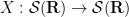
In contrast to previous notes, in this set of notes we shall focus exclusively on Fourier analysis in the one-dimensional setting for simplicity of notation, although all of the results here have natural extensions to higher dimensions. Depending on the physical context, one can view the physical domain as representing either space or time; we will mostly think in terms of the former interpretation, even though the standard terminology of “time-frequency analysis”, which we will make more prominent use of in later notes, clearly originates from the latter.

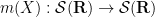
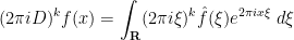
In previous notes we have often performed various localisations in either physical space or Fourier space , for instance in order to take advantage of the uncertainty principle. One can formalise these operations in terms of the functional calculus of two basic operations on Schwartz functions , the position operator defined by

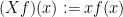
and the momentum operator , defined by

(The terminology comes from quantum mechanics, where it is customary to also insert a small constant on the right-hand side of (1) in accordance with de Broglie’s law. Such a normalisation is also used in several branches of mathematics, most notably semiclassical analysis and microlocal analysis, where it becomes profitable to consider the semiclassical limit , but we will not emphasise this perspective here.) The momentum operator can be viewed as the counterpart to the position operator, but in frequency space instead of physical space, since we have the standard identity

for any and . We observe that both operators are formally self-adjoint in the sense that

for all , where we use the Hermitian inner product

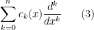
Clearly, for any polynomial of one real variable (with complex coefficients), the operator is given by the spatial multiplier operator

and similarly the operator is given by the Fourier multiplier operator

Inspired by this, if is any smooth function that obeys the derivative bounds

for all and (that is to say, all derivatives of grow at most polynomially), then we can define the spatial multiplier operator by the formula

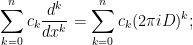
one can easily verify from several applications of the Leibniz rule that maps Schwartz functions to Schwartz functions. We refer to as the symbol of this spatial multiplier operator. In a similar fashion, we define the Fourier multiplier operator associated to the symbol by the formula

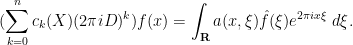
For instance, any constant coefficient linear differential operators can be written in this notation as

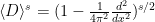
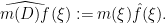
however there are many Fourier multiplier operators that are not of this form, such as fractional derivative operators for non-integer values of , which is a Fourier multiplier operator with symbol . It is also very common to use spatial cutoffs and Fourier cutoffs for various bump functions to localise functions in either space or frequency; we have seen several examples of such cutoffs in action in previous notes (often in the higher dimensional setting ).

We observe that the maps and are ring homomorphisms, thus for instance

and

for any obeying the derivative bounds (2); also is formally adjoint to in the sense that

for , and similarly for and . One can interpret these facts as part of the functional calculus of the operators , which can be interpreted as densely defined self-adjoint operators on . However, in this set of notes we will not develop the spectral theory necessary in order to fully set out this functional calculus rigorously.

In the field of PDE and ODE, it is also very common to study variable coefficient linear differential operators

where the are now functions of the spatial variable obeying the derivative bounds (2). A simple example is the quantum harmonic oscillator Hamiltonian . One can rewrite this operator in our notation as

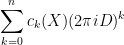
and so it is natural to interpret this operator as a combination of both the position operator and the momentum operator , where the symbol this operator is the function

Indeed, from the Fourier inversion formula

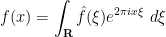
for any we have

and hence on multiplying by and summing we have

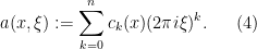
Inspired by this, we can introduce the Kohn-Nirenberg quantisation by defining the operator by the formula

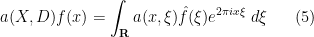
whenever and is any smooth function obeying the derivative bounds

for all and (note carefully that the exponent in on the right-hand side is required to be uniform in ). This quantisation clearly generalises both the spatial multiplier operators and the Fourier multiplier operators defined earlier, which correspond to the cases when the symbol is a function of only or only respectively. Thus we have combined the physical space and the frequency space into a single domain, known as phase space . The term “time-frequency analysis” encompasses analysis based on decompositions and other manipulations of phase space, in much the same way that “Fourier analysis” encompasses analysis based on decompositions and other manipulations of frequency space. We remark that the Kohn-Nirenberg quantization is not the only choice of quantization one could use; see Remark 19 below.

Exercise 1

• (i) Show that for obeying (6), that does indeed map to .
• (ii) Show that the symbol is uniquely determined by the operator . That is to say, if are two functions obeying (6) with for all , then . (Hint: apply to a suitable truncation of a plane wave and then take limits.)

In principle, the quantisations are potentially very useful for such tasks as inverting variable coefficient linear operators, or to localize a function simultaneously in physical and Fourier space. However, a fundamental difficulty arises: map from symbols to operators is now no longer a ring homomorphism, in particular

in general. Fundamentally, this is due to the fact that pointwise multiplication of symbols is a commutative operation, whereas the composition of operators such as and does not necessarily commute. This lack of commutativity can be measured by introducing the commutator

of two operators , and noting from the product rule that

(In the language of Lie groups and Lie algebras, this tells us that are (up to complex constants) the standard Lie algebra generators of the Heisenberg group.) From a quantum mechanical perspective, this lack of commutativity is the root cause of the uncertainty principle that prevents one from simultaneously localizing in both position and momentum past a certain point. Here is one basic way of formalising this principle:

Exercise 2 (Heisenberg uncertainty principle) For any and , show that

(Hint: evaluate the expression in two different ways and apply the Cauchy-Schwarz inequality.) Informally, this exercise asserts that the spatial uncertainty and the frequency uncertainty of a function obey the Heisenberg uncertainty relation .

Nevertheless, one still has the correspondence principle, which asserts that in certain regimes (which, with our choice of normalisations, corresponds to the high-frequency regime), quantum mechanics continues to behave like a commutative theory, and one can sometimes proceed as if the operators (and the various operators constructed from them) commute up to “lower order” errors. This can be formalised using the pseudodifferential calculus, which we give below the fold, in which we restrict the symbol to certain “symbol classes” of various orders (which then restricts to be pseudodifferential operators of various orders), and obtains approximate identities such as

where the error between the left and right-hand sides is of “lower order” and can in fact enjoys a useful asymptotic expansion. As a first approximation to this calculus, one can think of functions as having some sort of “phase space portrait” which somehow combines the physical space representation with its Fourier representation , and pseudodifferential operators behave approximately like “phase space multiplier operators” in this representation in the sense that

Unfortunately the uncertainty principle (or the non-commutativity of and ) prevents us from making these approximations perfectly precise, and it is not always clear how to even define a phase space portrait of a function precisely (although there are certain popular candidates for such a portrait, such as the FBI transform (also known as the Gabor transform in signal processing literature), or the Wigner quasiprobability distribution, each of which have some advantages and disadvantages). Nevertheless even if the concept of a phase space portrait is somewhat fuzzy, it is of great conceptual benefit both within mathematics and outside of it. For instance, the musical score one assigns a piece of music can be viewed as a phase space portrait of the sound waves generated by that music.

To complement the pseudodifferential calculus we have the basic Calderón-Vaillancourt theorem, which asserts that pseudodifferential operators of order zero are Calderón-Zygmund operators and thus bounded on for . The standard proof of this theorem is a classic application of one of the basic techniques in harmonic analysis, namely the exploitation of almost orthogonality; the proof we will give here will achieve this through the elegant device of the Cotlar-Stein lemma.

Pseudodifferential operators (especially when generalised to higher dimensions ) are a fundamental tool in the theory of linear PDE, as well as related fields such as semiclassical analysis, microlocal analysis, and geometric quantisation. There is an even wider class of operators that is also of interest, namely the Fourier integral operators, which roughly speaking not only approximately multiply the phase space portrait of a function by some multiplier , but also move the portrait around by a canonical transformation. However, the development of theory of these operators is beyond the scope of these notes; see for instance the texts of Hormander or Eskin.

This set of notes is only the briefest introduction to the theory of pseudodifferential operators. Many texts are available that cover the theory in more detail, for instance this text of Taylor.

254A, Notes 3: The large sieve and the Bombieri-Vinogradov theorem

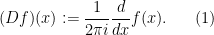
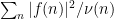
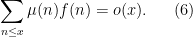
A fundamental and recurring problem in analytic number theory is to demonstrate the presence of cancellation in an oscillating sum, a typical example of which might be a correlation

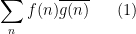
between two arithmetic functions and , which to avoid technicalities we will assume to be finitely supported (or that the variable is localised to a finite range, such as ). A key example to keep in mind for the purposes of this set of notes is the twisted von Mangoldt summatory function

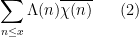
that measures the correlation between the primes and a Dirichlet character . One can get a “trivial” bound on such sums from the triangle inequality

for instance, from the triangle inequality and the prime number theorem we have

as . But the triangle inequality is insensitive to the phase oscillations of the summands, and often we expect (e.g. from the probabilistic heuristics from Supplement 4) to be able to improve upon the trivial triangle inequality bound by a substantial amount; in the best case scenario, one typically expects a “square root cancellation” that gains a factor that is roughly the square root of the number of summands. (For instance, for Dirichlet characters of conductor , it is expected from probabilistic heuristics that the left-hand side of (3) should in fact be for any .)

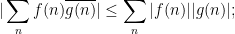
It has proven surprisingly difficult, however, to establish significant cancellation in many of the sums of interest in analytic number theory, particularly if the sums do not have a strong amount of algebraic structure (e.g. multiplicative structure) which allow for the deployment of specialised techniques (such as multiplicative number theory techniques). In fact, we are forced to rely (to an embarrassingly large extent) on (many variations of) a single basic tool to capture at least some cancellation, namely the Cauchy-Schwarz inequality. In fact, in many cases the classical case

considered by Cauchy, where at least one of is finitely supported, suffices for applications. Roughly speaking, the Cauchy-Schwarz inequality replaces the task of estimating a cross-correlation between two different functions , to that of measuring self-correlations between and itself, or and itself, which are usually easier to compute (albeit at the cost of capturing less cancellation). Note that the Cauchy-Schwarz inequality requires almost no hypotheses on the functions or , making it a very widely applicable tool.

There is however some skill required to decide exactly how to deploy the Cauchy-Schwarz inequality (and in particular, how to select and ); if applied blindly, one loses all cancellation and can even end up with a worse estimate than the trivial bound. For instance, if one tries to bound (2) directly by applying Cauchy-Schwarz with the functions and , one obtains the bound

The right-hand side may be bounded by , but this is worse than the trivial bound (3) by a logarithmic factor. This can be “blamed” on the fact that and are concentrated on rather different sets ( is concentrated on primes, while is more or less uniformly distributed amongst the natural numbers); but even if one corrects for this (e.g. by weighting Cauchy-Schwarz with some suitable “sieve weight” that is more concentrated on primes), one still does not do any better than (3). Indeed, the Cauchy-Schwarz inequality suffers from the same key weakness as the triangle inequality: it is insensitive to the phase oscillation of the factors .

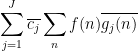
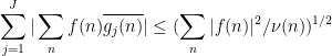
While the Cauchy-Schwarz inequality can be poor at estimating a single correlation such as (1), its power improves when considering an average (or sum, or square sum) of multiple correlations. In this set of notes, we will focus on one such situation of this type, namely that of trying to estimate a square sum

that measures the correlations of a single function with multiple other functions . One should think of the situation in which is a “complicated” function, such as the von Mangoldt function , but the are relatively “simple” functions, such as Dirichlet characters. In the case when the are orthonormal functions, we of course have the classical Bessel inequality:

Lemma 1 (Bessel inequality) Let be finitely supported functions obeying the orthonormality relationship

for all . Then for any function , we have

For sake of comparison, if one were to apply the Cauchy-Schwarz inequality (4) separately to each summand in (5), one would obtain the bound of , which is significantly inferior to the Bessel bound when is large. Geometrically, what is going on is this: the Cauchy-Schwarz inequality (4) is only close to sharp when and are close to parallel in the Hilbert space . But if are orthonormal, then it is not possible for any other vector to be simultaneously close to parallel to too many of these orthonormal vectors, and so the inner products of with most of the should be small. (See this previous blog post for more discussion of this principle.) One can view the Bessel inequality as formalising a repulsion principle: if correlates too much with some of the , then it does not have enough “energy” to have large correlation with the rest of the .

In analytic number theory applications, it is useful to generalise the Bessel inequality to the situation in which the are not necessarily orthonormal. This can be accomplished via the Cauchy-Schwarz inequality:

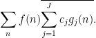
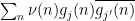
Proposition 2 (Generalised Bessel inequality) Let be finitely supported functions, and let be a non-negative function. Let be such that vanishes whenever vanishes, we have

for some sequence of complex numbers with , with the convention that vanishes whenever both vanish.

Note by relabeling that we may replace the domain here by any other at most countable set, such as the integers . (Indeed, one can give an analogue of this lemma on arbitrary measure spaces, but we will not do so here.) This result first appears in this paper of Boas.

Proof: We use the method of duality to replace the role of the function by a dual sequence . By the converse to Cauchy-Schwarz, we may write the left-hand side of (6) as

for some complex numbers with . Indeed, if all of the vanish, we can set the arbitrarily, otherwise we set to be the unit vector formed by dividing by its length. We can then rearrange this expression as

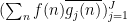
Applying Cauchy-Schwarz (dividing the first factor by and multiplying the second by , after first removing those for which vanish), this is bounded by

and the claim follows by expanding out the second factor.

Observe that Lemma 1 is a special case of Proposition 2 when and the are orthonormal. In general, one can expect Proposition 2 to be useful when the are almost orthogonal relative to , in that the correlations tend to be small when are distinct. In that case, one can hope for the diagonal term in the right-hand side of (6) to dominate, in which case one can obtain estimates of comparable strength to the classical Bessel inequality. The flexibility to choose different weights in the above proposition has some technical advantages; for instance, if is concentrated in a sparse set (such as the primes), it is sometimes useful to tailor to a comparable set (e.g. the almost primes) in order not to lose too much in the first factor . Also, it can be useful to choose a fairly “smooth” weight , in order to make the weighted correlations small.

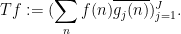
Remark 3 In harmonic analysis, the use of tools such as Proposition 2 is known as the method of almost orthogonality, or the method. The explanation for the latter name is as follows. For sake of exposition, suppose that is never zero (or we remove all from the domain for which vanishes). Given a family of finitely supported functions , consider the linear operator defined by the formula

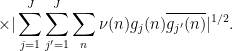
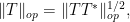
This is a bounded linear operator, and the left-hand side of (6) is nothing other than the norm of . Without any further information on the function other than its norm , the best estimate one can obtain on (6) here is clearly

where denotes the operator norm of .

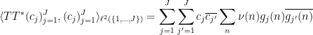
The adjoint is easily computed to be

The composition of and its adjoint is then given by

From the spectral theorem (or singular value decomposition), one sees that the operator norms of and are related by the identity

and as is a self-adjoint, positive semi-definite operator, the operator norm is also the supremum of the quantity

where ranges over unit vectors in . Putting these facts together, we obtain Proposition 2; furthermore, we see from this analysis that the bound here is essentially optimal if the only information one is allowed to use about is its norm.

For further discussion of almost orthogonality methods from a harmonic analysis perspective, see Chapter VII of this text of Stein.

Exercise 4 Under the same hypotheses as Proposition 2, show that

as well as the variant inequality

Proposition 2 has many applications in analytic number theory; for instance, we will use it in later notes to control the large value of Dirichlet series such as the Riemann zeta function. One of the key benefits is that it largely eliminates the need to consider further correlations of the function (other than its self-correlation relative to , which is usually fairly easy to compute or estimate as is usually chosen to be relatively simple); this is particularly useful if is a function which is significantly more complicated to analyse than the functions . Of course, the tradeoff for this is that one now has to deal with the coefficients , which if anything are even less understood than , since literally the only thing we know about these coefficients is their square sum . However, as long as there is enough almost orthogonality between the , one can estimate the by fairly crude estimates (e.g. triangle inequality or Cauchy-Schwarz) and still get reasonably good estimates.

In this set of notes, we will use Proposition 2 to prove some versions of the large sieve inequality, which controls a square-sum of correlations

of an arbitrary finitely supported function with various additive characters (where ), or alternatively a square-sum of correlations

of with various primitive Dirichlet characters ; it turns out that one can prove a (slightly sub-optimal) version of this inequality quite quickly from Proposition 2 if one first prepares the sum by inserting a smooth cutoff with well-behaved Fourier transform. The large sieve inequality has many applications (as the name suggests, it has particular utility within sieve theory). For the purposes of this set of notes, though, the main application we will need it for is the Bombieri-Vinogradov theorem, which in a very rough sense gives a prime number theorem in arithmetic progressions, which, “on average”, is of strength comparable to the results provided by the Generalised Riemann Hypothesis (GRH), but has the great advantage of being unconditional (it does not require any unproven hypotheses such as GRH); it can be viewed as a significant extension of the Siegel-Walfisz theorem from Notes 2. As we shall see in later notes, the Bombieri-Vinogradov theorem is a very useful ingredient in sieve-theoretic problems involving the primes.

There is however one additional important trick, beyond the large sieve, which we will need in order to establish the Bombieri-Vinogradov theorem. As it turns out, after some basic manipulations (and the deployment of some multiplicative number theory, and specifically the Siegel-Walfisz theorem), the task of proving the Bombieri-Vinogradov theorem is reduced to that of getting a good estimate on sums that are roughly of the form

for some primitive Dirichlet characters . This looks like the type of sum that can be controlled by the large sieve (or by Proposition 2), except that this is an ordinary sum rather than a square sum (i.e., an norm rather than an norm). One could of course try to control such a sum in terms of the associated square-sum through the Cauchy-Schwarz inequality, but this turns out to be very wasteful (it loses a factor of about ). Instead, one should try to exploit the special structure of the von Mangoldt function , in particular the fact that it can be expressible as a Dirichlet convolution of two further arithmetic sequences (or as a finite linear combination of such Dirichlet convolutions). The reason for introducing this convolution structure is through the basic identity

for any finitely supported sequences , as can be easily seen by multiplying everything out and using the completely multiplicative nature of . (This is the multiplicative analogue of the well-known relationship between ordinary convolution and Fourier coefficients.) This factorisation, together with yet another application of the Cauchy-Schwarz inequality, lets one control (7) by square-sums of the sort that can be handled by the large sieve inequality.

As we have seen in Notes 1, the von Mangoldt function does indeed admit several factorisations into Dirichlet convolution type, such as the factorisation . One can try directly inserting this factorisation into the above strategy; it almost works, however there turns out to be a problem when considering the contribution of the portion of or that is supported at very small natural numbers, as the large sieve loses any gain over the trivial bound in such settings. Because of this, there is a need for a more sophisticated decomposition of into Dirichlet convolutions which are non-degenerate in the sense that are supported away from small values. (As a non-example, the trivial factorisation would be a totally inappropriate factorisation for this purpose.) Fortunately, it turns out that through some elementary combinatorial manipulations, some satisfactory decompositions of this type are available, such as the Vaughan identity and the Heath-Brown identity. By using one of these identities we will be able to complete the proof of the Bombieri-Vinogradov theorem. (These identities are also useful for other applications in which one wishes to control correlations between the von Mangoldt function and some other sequence; we will see some examples of this in later notes.)

For further reading on these topics, including a significantly larger number of examples of the large sieve inequality, see Chapters 7 and 17 of Iwaniec and Kowalski.

Remark 5 We caution that the presentation given in this set of notes is highly ahistorical; we are using modern streamlined proofs of results that were first obtained by more complicated arguments.

The Katai-Bourgain-Sarnak-Ziegler orthogonality criterion

One of the basic problems in analytic number theory is to estimate sums of the form

as , where ranges over primes and is some explicit function of interest (e.g. a linear phase function for some real number ). This is essentially the same task as obtaining estimates on the sum

where is the von Mangoldt function. If is bounded, , then from the prime number theorem one has the trivial bound

but often (when is somehow “oscillatory” in nature) one is seeking the refinement

or equivalently

Thanks to identities such as

where is the Möbius function, refinements such as (1) are similar in spirit to estimates of the form

Unfortunately, the connection between (1) and (4) is not particularly tight; roughly speaking, one needs to improve the bounds in (4) (and variants thereof) by about two factors of before one can use identities such as (3) to recover (1). Still, one generally thinks of (1) and (4) as being “morally” equivalent, even if they are not formally equivalent.

When is oscillating in a sufficiently “irrational” way, then one standard way to proceed is the method of Type I and Type II sums, which uses truncated versions of divisor identities such as (3) to expand out either (1) or (4) into linear (Type I) or bilinear sums (Type II) with which one can exploit the oscillation of . For instance, Vaughan’s identity lets one rewrite the sum in (1) as the sum of the Type I sum

the Type I sum

the Type II sum

and the error term , whenever are parameters, and are the sequences

and

Similarly one can express (4) as the Type I sum

the Type II sum

and the error term , whenever with , and is the sequence

After eliminating troublesome sequences such as via Cauchy-Schwarz or the triangle inequality, one is then faced with the task of estimating Type I sums such as

or Type II sums such as

for various . Here, the trivial bound is , but due to a number of logarithmic inefficiencies in the above method, one has to obtain bounds that are more like for some constant (e.g. ) in order to end up with an asymptotic such as (1) or (4).

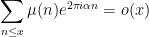
However, in a recent paper of Bourgain, Sarnak, and Ziegler, it was observed that as long as one is only seeking the Mobius orthogonality (4) rather than the von Mangoldt orthogonality (1), one can avoid losing any logarithmic factors, and rely purely on qualitative equidistribution properties of . A special case of their orthogonality criterion (which actually dates back to an earlier paper of Katai, as was pointed out to me by Nikos Frantzikinakis) is as follows:

Proposition 1 (Orthogonality criterion) Let be a bounded function such that

for any distinct primes (where the decay rate of the error term may depend on and ). Then

Actually, the Bourgain-Sarnak-Ziegler paper establishes a more quantitative version of this proposition, in which can be replaced by an arbitrary bounded multiplicative function, but we will content ourselves with the above weaker special case. (See also these notes of Harper, which uses the Katai argument to give a slightly weaker quantitative bound in the same spirit.) This criterion can be viewed as a multiplicative variant of the classical van der Corput lemma, which in our notation asserts that if one has for each fixed non-zero .

As a sample application, Proposition 1 easily gives a proof of the asymptotic

for any irrational . (For rational , this is a little trickier, as it is basically equivalent to the prime number theorem in arithmetic progressions.) The paper of Bourgain, Sarnak, and Ziegler also apply this criterion to nilsequences (obtaining a quick proof of a qualitative version of a result of Ben Green and myself, see these notes of Ziegler for details) and to horocycle flows (for which no Möbius orthogonality result was previously known).

Informally, the connection between (5) and (6) comes from the multiplicative nature of the Möbius function. If (6) failed, then exhibits strong correlation with ; by change of variables, we then expect to correlate with and to correlate with , for “typical” at least. On the other hand, since is multiplicative, exhibits strong correlation with . Putting all this together (and pretending correlation is transitive), this would give the claim (in the contrapositive). Of course, correlation is not quite transitive, but it turns out that one can use the Cauchy-Schwarz inequality as a substitute for transitivity of correlation in this case.

I will give a proof of Proposition 1 below the fold (which is not quite based on the argument in the above mentioned paper, but on a variant of that argument communicated to me by Tamar Ziegler, and also independently discovered by Adam Harper). The main idea is to exploit the following observation: if is a “large” but finite set of primes (in the sense that the sum is large), then for a typical large number (much larger than the elements of ), the number of primes in that divide is pretty close to :

A more precise formalisation of this heuristic is provided by the Turan-Kubilius inequality, which is proven by a simple application of the second moment method.

In particular, one can sum (7) against and obtain an approximation

that approximates a sum of by a bunch of sparser sums of . Since

we see (heuristically, at least) that in order to establish (4), it would suffice to establish the sparser estimates

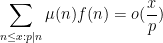
for all (or at least for “most” ).

Now we make the change of variables . As the Möbius function is multiplicative, we usually have . (There is an exception when is divisible by , but this will be a rare event and we will be able to ignore it.) So it should suffice to show that

for most . However, by the hypothesis (5), the sequences are asymptotically orthogonal as varies, and this claim will then follow from a Cauchy-Schwarz argument.

The Cotlar-Stein lemma

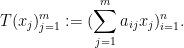
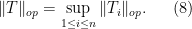
A basic problem in harmonic analysis (as well as in linear algebra, random matrix theory, and high-dimensional geometry) is to estimate the operator norm of a linear map between two Hilbert spaces, which we will take to be complex for sake of discussion. Even the finite-dimensional case is of interest, as this operator norm is the same as the largest singular value of the matrix associated to .

In general, this operator norm is hard to compute precisely, except in special cases. One such special case is that of a diagonal operator, such as that associated to an diagonal matrix . In this case, the operator norm is simply the supremum norm of the diagonal coefficients:

A variant of (1) is Schur’s test, which for simplicity we will phrase in the setting of finite-dimensional operators 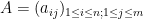given by a matrix via the usual formula

A simple version of this test is as follows: if all the absolute row sums and columns sums of are bounded by some constant , thus

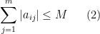
for all and

for all , then

(note that this generalises (the upper bound in) (1).) Indeed, to see (4), it suffices by duality and homogeneity to show that

whenever and are sequences with ; but this easily follows from the arithmetic mean-geometric mean inequality

and (2), (3).

Schur’s test (4) (and its many generalisations to weighted situations, or to Lebesgue or Lorentz spaces) is particularly useful for controlling operators in which the role of oscillation (as reflected in the phase of the coefficients , as opposed to just their magnitudes ) is not decisive. However, it is of limited use in situations that involve a lot of cancellation. For this, a different test, known as the Cotlar-Stein lemma, is much more flexible and powerful. It can be viewed in a sense as a non-commutative variant of Schur’s test (4) (or of (1)), in which the scalar coefficients or are replaced by operators instead.

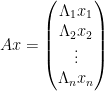
To illustrate the basic flavour of the result, let us return to the bound (1), and now consider instead a block-diagonal matrix

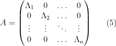
where each is now a matrix, and so is an matrix with . Then we have

Indeed, the lower bound is trivial (as can be seen by testing on vectors which are supported on the block of coordinates), while to establish the upper bound, one can make use of the orthogonal decomposition

to decompose an arbitrary vector as

with , in which case we have

and the upper bound in (6) then follows from a simple computation.

The operator associated to the matrix in (5) can be viewed as a sum , where each corresponds to the block of , in which case (6) can also be written as

When is large, this is a significant improvement over the triangle inequality, which merely gives

The reason for this gain can ultimately be traced back to the “orthogonality” of the ; that they “occupy different columns” and “different rows” of the range and domain of . This is obvious when viewed in the matrix formalism, but can also be described in the more abstract Hilbert space operator formalism via the identities

and

whenever . (The first identity asserts that the ranges of the are orthogonal to each other, and the second asserts that the coranges of the (the ranges of the adjoints ) are orthogonal to each other.) By replacing (7) with a more abstract orthogonal decomposition into these ranges and coranges, one can in fact deduce (8) directly from (9) and (10).

The Cotlar-Stein lemma is an extension of this observation to the case where the are merely almost orthogonal rather than orthogonal, in a manner somewhat analogous to how Schur’s test (partially) extends (1) to the non-diagonal case. Specifically, we have

Lemma 1 (Cotlar-Stein lemma) Let be a finite sequence of bounded linear operators from one Hilbert space to another , obeying the bounds

and

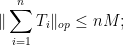
for all and some (compare with (2), (3)). Then one has

Note from the basic identity

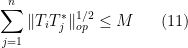
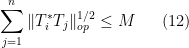
that the hypothesis (11) (or (12)) already gives the bound

on each component of , which by the triangle inequality gives the inferior bound

the point of the Cotlar-Stein lemma is that the dependence on in this bound is eliminated in (13), which in particular makes the bound suitable for extension to the limit (see Remark 1 below).

The Cotlar-Stein lemma was first established by Cotlar in the special case of commuting self-adjoint operators, and then independently by Cotlar and Stein in full generality, with the proof appearing in a subsequent paper of Knapp and Stein.

The Cotlar-Stein lemma is often useful in controlling operators such as singular integral operators or pseudo-differential operators which “do not mix scales together too much”, in that operators map functions “that oscillate at a given scale ” to functions that still mostly oscillate at the same scale . In that case, one can often split into components which essentically capture the scale behaviour, and understanding boundedness properties of then reduces to establishing the boundedness of the simpler operators (and of establishing a sufficient decay in products such as or when and are separated from each other). In some cases, one can use Fourier-analytic tools such as Littlewood-Paley projections to generate the , but the true power of the Cotlar-Stein lemma comes from situations in which the Fourier transform is not suitable, such as when one has a complicated domain (e.g. a manifold or a non-abelian Lie group), or very rough coefficients (which would then have badly behaved Fourier behaviour). One can then select the decomposition in a fashion that is tailored to the particular operator , and is not necessarily dictated by Fourier-analytic considerations.

Once one is in the almost orthogonal setting, as opposed to the genuinely orthogonal setting, the previous arguments based on orthogonal projection seem to fail completely. Instead, the proof of the Cotlar-Stein lemma proceeds via an elegant application of the tensor power trick (or perhaps more accurately, the power method), in which the operator norm of is understood through the operator norm of a large power of (or more precisely, of its self-adjoint square or ). Indeed, from an iteration of (14) we see that for any natural number , one has

To estimate the right-hand side, we expand out the right-hand side and apply the triangle inequality to bound it by

Recall that when we applied the triangle inequality directly to , we lost a factor of in the final estimate; it will turn out that we will lose a similar factor here, but this factor will eventually be attenuated into nothingness by the tensor power trick.

To bound (17), we use the basic inequality in two different ways. If we group the product in pairs, we can bound the summand of (17) by

On the other hand, we can group the product by pairs in another way, to obtain the bound of

We bound and crudely by using (15). Taking the geometric mean of the above bounds, we can thus bound (17) by

If we then sum this series first in , then in , then moving back all the way to , using (11) and (12) alternately, we obtain a final bound of

for (16). Taking roots, we obtain

Sending , we obtain the claim.

Remark 1 As observed in a number of places (see e.g. page 318 of Stein’s book, or this paper of Comech, the Cotlar-Stein lemma can be extended to infinite sums (with the obvious changes to the hypotheses (11), (12)). Indeed, one can show that for any , the sum is unconditionally convergent in (and furthermore has bounded -variation), and the resulting operator is a bounded linear operator with an operator norm bound on .

Remark 2 If we specialise to the case where all the are equal, we see that the bound in the Cotlar-Stein lemma is sharp, at least in this case. Thus we see how the tensor power trick can convert an inefficient argument, such as that obtained using the triangle inequality or crude bounds such as (15), into an efficient one.

Remark 3 One can prove Schur’s test by a similar method. Indeed, starting from the inequality

(which follows easily from the singular value decomposition), we can bound by

Estimating the other two terms in the summand by , and then repeatedly summing the indices one at a time as before, we obtain

and the claim follows from the tensor power trick as before. On the other hand, in the converse direction, I do not know of any way to prove the Cotlar-Stein lemma that does not basically go through the tensor power argument.

Distinguished Lecture Series I: Elias Stein, “Singular Integrals and Several Complex Variables: Some New Perspectives”

The first Distinguished Lecture Series at UCLA for this academic year is given by Elias Stein (who, incidentally, was my graduate student advisor), who is lecturing on “Singular Integrals and Several Complex Variables: Some New Perspectives“.  The first lecture was a historical (and non-technical) survey of modern harmonic analysis (which, amazingly, was compressed into half an hour), followed by an introduction as to how this theory is currently in the process of being adapted to handle the basic analytical issues in several complex variables, a topic which in many ways is still only now being developed.  The second and third lectures will focus on these issues in greater depth.

As usual, any errors here are due to my transcription and interpretation of the lecture.

[Update, Oct 27: The slides from the talk are now available here.]

Tricks Wiki article: The tensor power trick

As many readers may already know, my good friend and fellow mathematical blogger Tim Gowers, having wrapped up work on the Princeton Companion to Mathematics (which I believe is now in press), has begun another mathematical initiative, namely a “Tricks Wiki” to act as a repository for mathematical tricks and techniques.    Tim has already started the ball rolling with several seed articles on his own blog, and asked me to also contribute some articles.  (As I understand it, these articles will be migrated to the Wiki in a few months, once it is fully set up, and then they will evolve with edits and contributions by anyone who wishes to pitch in, in the spirit of Wikipedia; in particular, articles are not intended to be permanently authored or signed by any single contributor.)

So today I’d like to start by extracting some material from an old post of mine on “Amplification, arbitrage, and the tensor power trick” (as well as from some of the comments), and converting it to the Tricks Wiki format, while also taking the opportunity to add a few more examples.

Title: The tensor power trick

Quick description: If one wants to prove an inequality for some non-negative quantities X, Y, but can only see how to prove a quasi-inequality that loses a multiplicative constant C, then try to replace all objects involved in the problem by “tensor powers” of themselves and apply the quasi-inequality to those powers.  If all goes well, one can show that for all , with a constant C which is independent of M, which implies that as desired by taking roots and then taking limits as .