The parity problem is a notorious problem in sieve theory: this theory was invented in order to count prime patterns of various types (e.g. twin primes), but despite superb success in obtaining upper bounds on the number of such patterns, it has proven to be somewhat disappointing in obtaining lower bounds. [Sieves can also be used to study many other things than primes, of course, but we shall focus only on primes in this post.] Even the task of reproving Euclid’s theorem – that there are infinitely many primes – seems to be extremely difficult to do by sieve theoretic means, unless one of course injects into the theory an estimate at least as strong as Euclid’s theorem (e.g. the prime number theorem). The main obstruction is the parity problem: even assuming such strong hypotheses as the Elliott-Halberstam conjecture (a sort of “super-generalised Riemann Hypothesis” for sieves), sieve theory is largely (but not completely) unable to distinguish numbers with an odd number of prime factors from numbers with an even number of prime factors. This “parity barrier” has been broken for some select patterns of primes by injecting some powerful non-sieve theory methods into the subject, but remains a formidable obstacle in general.
I’ll discuss the parity problem in more detail later in this post, but I want to first discuss how sieves work [drawing in part on some excellent unpublished lecture notes of Iwaniec]; the basic ideas are elementary and conceptually simple, but there are many details and technicalities involved in actually executing these ideas, and which I will try to suppress for sake of exposition.
Let’s consider a basic question in prime number theory, namely how to count the number of primes in a given range, say between N and 2N for some large integer N. (This problem is more or less equivalent to that of counting primes between 1 and N, thanks to dyadic decomposition, but by keeping the magnitude of all numbers comparable to N we can simplify some (very minor) technicalities.) Of course, we know that this particular question can be settled fairly satisfactorily (the answer is  ) using known facts about the Riemann zeta function, but let us pretend for now that we do not know about this function. (Once one moves to slightly more complicated additive questions about the primes, such as counting twin primes, the theory of the zeta function and its relatives becomes much less powerful, even assuming such things as the Riemann hypothesis; the problem is that these functions are measuring the multiplicative structure of the primes rather than the additive structure.)
The set of primes does not appear to have enough usable structure in order to perform such counts quickly. However, one can count other sets of numbers between N and 2N with much more ease. For instance, the set of integers between N and 2N can be easily counted with small error:
![| \{ n \in [N,2N]: n \hbox{ integer} \}| = N + O(1)](https://s0.wp.com/latex.php?latex=%7C+%5C%7B+n+%5Cin+%5BN%2C2N%5D%3A+n+%5Chbox%7B+integer%7D+%5C%7D%7C+%3D+N+%2B+O%281%29&bg=ffffff&fg=545454&s=0&c=20201002) ;
;
the error term O(1) in this case is in fact just 1. Similarly, we can count, say, the number of odd numbers between N and 2N,
![| \{ n \in [N,2N]: n \hbox{ odd} \}| = \frac{1}{2} N + O(1)](https://s0.wp.com/latex.php?latex=%7C+%5C%7B+n+%5Cin+%5BN%2C2N%5D%3A+n+%5Chbox%7B+odd%7D+%5C%7D%7C+%3D+%5Cfrac%7B1%7D%7B2%7D+N+%2B+O%281%29&bg=ffffff&fg=545454&s=0&c=20201002) ,
,
simply because the set of odd numbers has density  and is periodic of period 2. The error term O(1) now depends on the parity of N. More generally, we can count any given residue class in [N,2N] to a reasonable accuracy:
![| \{ n \in [N,2N]: n = a\mod q \}| = \frac{1}{q} N + O(1)](https://s0.wp.com/latex.php?latex=%7C+%5C%7B+n+%5Cin+%5BN%2C2N%5D%3A+n+%3D+a%5Cmod+q+%5C%7D%7C+%3D+%5Cfrac%7B1%7D%7Bq%7D+N+%2B+O%281%29&bg=ffffff&fg=545454&s=0&c=20201002) ,
,
where the error term is now more complicated, and depends on what N is doing modulo q. This estimate is quite good as long as q is small compared with N, but once q is very large, the error term O(1) can begin to overwhelm the main term (especially if the main term is going to appear in a delicate summation with lots of cancellation). In general, any summation involving the main term N/q will be relatively easy to manipulate (because it is essentially multiplicative in q, and thus amenable to all the methods of multiplicative number theory, in particular Euler products and zeta functions); it is the error term O(1) which causes all the difficulty.
Once we have figured out how to count these basic sets, we can also count some combinations of these sets, as long as these combinations are simple enough. For instance, suppose we want to count
![| \{ n \in [N,2N]: n \hbox{ coprime to } 2,3 \}|](https://s0.wp.com/latex.php?latex=%7C+%5C%7B+n+%5Cin+%5BN%2C2N%5D%3A+n+%5Chbox%7B+coprime+to+%7D+2%2C3+%5C%7D%7C&bg=ffffff&fg=545454&s=0&c=20201002) (1).
(1).
Well, we know that the total number of integers in [N,2N] is N+O(1). Of this set, we know that  are not coprime to 2 (i.e. divisible by 2), and that
  are not coprime to 3. So we should subtract those two sets from the original set, leaving
  . But the numbers which are divisible by both 2 and 3 (i.e. divisible by 6) have been subtracted twice, so we have to put them back in; this adds in another
  , giving a final count of for the quantity (1); this is of course a simple instance of the inclusion-exclusion principle in action. An alternative way to estimate (1) is to use the Chinese remainder theorem to rewrite (1) as
![|\{ n \in [N,2N]: n = 1,5 \mod 6 \}|](https://s0.wp.com/latex.php?latex=%7C%5C%7B+n+%5Cin+%5BN%2C2N%5D%3A+n+%3D+1%2C5+%5Cmod+6+%5C%7D%7C&bg=ffffff&fg=545454&s=0&c=20201002)
and use our ability to count residue classes modulo 6 to get the same final count of (though the precise bound on the error term will be slightly different). For very small moduli such as 2 and 3, the Chinese remainder theorem is quite efficient, but it is somewhat rigid, and for higher moduli (e.g. for moduli much larger than  ) it turns out that the more flexible inclusion-exclusion principle gives much better results (after applying some tricks to optimise the efficiency of that principle).
We can of course continue the example in (1), counting the numbers in [N,2N] which are coprime to 2,3,5,7, etc., which by the sieve of Eratosthenes will eventually give us a count for the primes in [N,2N], but let us pause for a moment to look at the larger picture. We have seen that some sets in [N,2N] are fairly easy to count accurately (e.g. residue classes with small modulus), and others are not (e.g. primes, twin primes). What is the defining characteristic of the former types of sets? One reasonable answer is that the sets that are easy to count are low-complexity, but this is a rather vaguely defined term. I would like to propose instead that sets (or more generally, weight functions – see below) are easy to count (or at least estimate) whenever they are smooth in a certain sense to be made more precise shortly. This terminology comes from harmonic analysis rather than from number theory (though number theory does have the related concept of a smooth number), so I will now digress a little bit to talk about smoothness, as it seems to me that this concept implicitly underlies the basic strategy of sieve theory.
Instead of talking about the problem of (approximately) counting a given set in [N,2N], let us consider instead the analogous problem of (approximately) computing the area of a given region E (e.g. a solid ellipse) in the unit square ![{}[0,1]^2](https://s0.wp.com/latex.php?latex=%7B%7D%5B0%2C1%5D%5E2&bg=ffffff&fg=545454&s=0&c=20201002) . As we are taught in high school, one way to do this is to subdivide the square into smaller squares, e.g. squares of length
. As we are taught in high school, one way to do this is to subdivide the square into smaller squares, e.g. squares of length  for some n, and count how many of these small squares lie completely or partially in the set E, and multiply by the area of each square; this is of course the prelude to the Riemann integral. It works well as long as the set E is “smooth” in the sense that most of the small squares are either completely inside or completely outside the set E, with few borderline cases; this notion of smoothness can also be viewed as a quantitative version of Lebesgue measurability. Another way of saying this is that if one wants to determine whether a given point (x,y) lies in E, it is usually enough just to compute x and y to the first n significant digits in the decimal expansion.
Now we return to counting sets in [N,2N]. One can also define the notion of a “smooth set” here by again using the most significant digits of the numbers n in the interval [N,2N]; for instance, the set [1.1 N, 1.2 N] would be quite smooth, as one would be fairly confident whether n would lie in this set or not after looking at just the top two or three significant digits. However, with this “Euclidean” or “Archimedean” notion of smoothness, sets such as the primes or the odd numbers are certainly not smooth. However, things look a lot better if we change the metric, or (more informally) if we redefine what “most significant digit” is. For instance, if we view the last digit in the base 10 expansion of a number n (i.e. the value of  ) as the most significant one, rather than the first – or more precisely, if we use the 10-adic metric intead of the Euclidean one, thus embedding the integers into
  rather than into
  – then the odd numbers become quite smooth (the most significant digit completely determines membership in this set). The primes in [N,2N] are not fully smooth, but they do exhibit some partial smoothness; indeed, if the most significant digit is 0, 2, 4, 5, 6, or 8, this fully determines membership in the set, though if the most significant digit is 1, 3, 7, or 9 then one only has partial information on membership in the set.
Now, the 10-adic metric is not fully satisfactory for characterising the elusive concept of number-theoretic “smoothness”. For instance, the multiples of 3 should be a smooth set, but this is not the case in the 10-adic metric (one really needs all the digits before one can be sure whether a number is a multiple of 3!). Also, we have the problem that the set [N/2,N] itself is now no longer smooth. This can be fixed by working not with just the Euclidean metric or a single n-adic metric, but with the product of all the n-adic metrics and the Euclidean metric at once. Actually, thanks to the Chinese remainder theorem, it is enough to work with the product of the p-adic metrics for primes p and the Euclidean metric, thus embedding the integers in the integer adele ring  . For some strange reason, this adele ring is not explicitly used in most treatments of sieve theory, despite its obvious relevance (and despite the amply demonstrated usefulness of this ring in algebraic number theory or in the theory of L-functions, as exhibited for instance by Tate’s thesis). At any rate, we are only using the notion of “smoothness” in a very informal sense, and so we will not need the full formalism of the adeles here. Suffice to say that a set of integers in [N,2N] is “smooth” if membership in that set can be largely determined by its most significant digits in the Euclidean sense, and also in the p-adic senses for small p; roughly speaking, this means that this set is approximately the pullback of some “low complexity” set in the adele ring – a set which can be efficiently fashioned out of a few of basic sets which generate the topology and
  -algebra of that ring. (Actually, in many applications of sieve theory, we only need to deal with moduli q which are square-free, which means that we can replace the p-adics
  with the cyclic group
  , and so it is now just the residues mod p for small p, together with the Euclidean most significant digits, which should control what smooth sets are; thus the adele ring has been replaced by the product
  .)
.)
Let us now return back to sieve theory, and the task of counting “rough” sets such as the primes in [N,2N]. Since we know how to accurately count “smooth” sets such as ![\{ n \in [N,2N]: n = a \mod q \}](https://s0.wp.com/latex.php?latex=%5C%7B+n+%5Cin+%5BN%2C2N%5D%3A+n+%3D+a+%5Cmod+q+%5C%7D&bg=ffffff&fg=545454&s=0&c=20201002) with q small, one can try to describe the rough set of primes as some sort of combination of smooth sets. The most direct implementation of this idea is the sieve of Eratosthenes; if one then tries to compute the number of primes using the inclusion-exclusion principle, one obtains the Legendre sieve; we implicitly used this idea previously when counting the quantity (1). However, the number of terms in the inclusion-exclusion formula is very large; if one runs the sieve of Eratosthenes for k steps (i.e. sieving out multiples of the first k primes), there are basically
with q small, one can try to describe the rough set of primes as some sort of combination of smooth sets. The most direct implementation of this idea is the sieve of Eratosthenes; if one then tries to compute the number of primes using the inclusion-exclusion principle, one obtains the Legendre sieve; we implicitly used this idea previously when counting the quantity (1). However, the number of terms in the inclusion-exclusion formula is very large; if one runs the sieve of Eratosthenes for k steps (i.e. sieving out multiples of the first k primes), there are basically  terms in the inclusion-exclusion formula, leading to an error term which in the worst case could be of size
  . A related issue is that the modulus q in many of the terms in the Legendre sieve become quite large – as large as the product of the first k primes (which turns out to be roughly
  in size). Since the set one is trying to count is only of size N, we thus see that the Legendre sieve becomes useless after just or so steps of the Eratosthenes sieve, which is well short of what one needs to accurately count primes (which requires that one uses
  or so steps). More generally, “exact” sieves such as the Legendre sieve are useful for any situation involving only a logarithmically small number of moduli, but are unsuitable for sieving with much larger numbers of moduli.
One can describe the early development of sieve theory as a concerted effort to rectify the drawbacks of the Legendre sieve. The first main idea here is to not try to compute the size of the rough set exactly – as this is too “expensive” in terms of the number of smooth sets required to fully describe the rough set – but instead to just settle for upper or lower bounds on the size of this set, which use fewer smooth sets. There is thus a tradeoff between how well the bounds approximate the original set, and how well one can compute the bounds themselves; by selecting various parameters appropriately one can optimise this tradeoff and obtain a final bound which is non-trivial but not completely exact. For instance, in using the Legendre sieve to try to count primes between N and 2N, one can instead use that sieve to count the much larger set of numbers between N and 2N which are coprime to the first k primes, thus giving an upper bound for the primes between N and 2N. It turns out that the optimal value of k here is roughly or so (after this, the error terms in the Legendre sieve get out of hand), and give an upper bound of  for the number of primes between N and 2N – somewhat far from the truth (which is
  ), but still non-trivial.
In a similar spirit, one can work with various truncated and approximate versions of the inclusion-exclusion formula which involve fewer terms. For instance, to estimate the cardinality  of the union of k sets, one can replace the inclusion-exclusion formula

 (2)
(2)
by the obvious upper bound

(also known as the union bound), or by the slightly less obvious lower bound

More generally, if one takes the first n terms on the right-hand side of (2), this will be an upper bound for the left-hand side for odd n and a lower bound for even n. These inequalities, known as the Bonferroni inequalities, are a nice exercise to prove: they are equivalent to the observation that in the binomial identity

for any  , the partial sums on the right-hand side alternate in sign between non-negative and non-positive. If one inserts these inequalities into the Legendre sieve and optimises the parameter, one can improve the upper bound for the number of primes in [N,2N] to
  , which is significantly closer to the truth. Unfortunately, this method does not provide any lower bound other than the trivial bound of 0; either the main term is negative, or the error term swamps the main term. A similar argument was used by Brun to show that the number of twin primes in [N,2N] was
  (again, the truth is conjectured to be
  ), which implied his famous theorem that the sum of reciprocals of the twin primes is convergent.
The full inclusion-exclusion expansion is a sum over terms, which one can view as binary strings of 0s and 1s of length k. In the Bonferroni inequalities, one only sums over a smaller collection of strings, namely the Hamming ball of strings which only involve n or fewer 1s. There are other collections of strings one can use which lead to upper or lower bounds; one can imagine revealing such a string one digit at a time and then deciding whether to keep or toss out this string once some threshold rule is reached. There are various ways to select these thresholding rules, leading to the family of combinatorial sieves. One particularly efficient such rule is similar to that given by the Bonferroni inequalities, but instead of using the number of 1s in a string to determine membership in the summation, one uses a weighted number of 1s (giving large primes more weight than small primes, because they tend to increase the modulus too quickly and thus should be removed from the sum sooner than the small primes). This leads to the beta sieve, which for instance gives the correct order of magnitude of  for the number of primes in [N,2N] or
  for the number of twin primes in [N,2N]. This sieve is also powerful enough to give lower bounds, but only if one stops the sieve somewhat early, thus enlarging the set of primes to a set of almost primes (numbers which are coprime to all numbers less than a certain threshold, and thus have a bounded number of prime factors). For instance, this sieve can show that there are an infinite number of twins
  , each of which has at most nine prime factors (the nine is not optimal, but to get better results requires much more work).
There seems however to be a limit as to what can be accomplished by purely combinatorial sieves. The problem stems from the “binary” viewpoint of such sieves: any given term in the inclusion-exclusion expansion is either included or excluded from the sieve upper or lower bound, and there is no middle ground. This leads to the next main idea in modern sieve theory, which is to work not with the cardinalities of sets in [N,2N], but rather with more flexible notion of sums of weight functions (real-valued functions on [N,2N]). The starting point is the obvious formula
![|A| = \sum_{n \in [N, 2N]} 1_A(n)](https://s0.wp.com/latex.php?latex=%7CA%7C+%3D+%5Csum_%7Bn+%5Cin+%5BN%2C+2N%5D%7D+1_A%28n%29&bg=ffffff&fg=545454&s=0&c=20201002)
for the cardinality of a set A in [N,2N], where  is the indicator function of the set A. Applying this to smooth sets such as
 ![\{ n \in [N,2N]: n = a \mod q\}](https://s0.wp.com/latex.php?latex=%5C%7B+n+%5Cin+%5BN%2C2N%5D%3A+n+%3D+a+%5Cmod+q%5C%7D&bg=ffffff&fg=545454&s=0&c=20201002) , we obtain
, we obtain
![\sum_{n \in [N, 2N]} 1_{n=a \mod q}(n) = \frac{N}{q} + O(1)](https://s0.wp.com/latex.php?latex=%5Csum_%7Bn+%5Cin+%5BN%2C+2N%5D%7D+1_%7Bn%3Da+%5Cmod+q%7D%28n%29+%3D+%5Cfrac%7BN%7D%7Bq%7D+%2B+O%281%29&bg=ffffff&fg=545454&s=0&c=20201002) ;
;
in particular, specialising to the 0 residue class a = 0 (which is the residue class of importance for counting primes) we have
![\sum_{n \in [N,2N]} 1_{d|n}(n) = \frac{N}{d} + O(1)](https://s0.wp.com/latex.php?latex=%5Csum_%7Bn+%5Cin+%5BN%2C2N%5D%7D+1_%7Bd%7Cn%7D%28n%29+%3D+%5Cfrac%7BN%7D%7Bd%7D+%2B+O%281%29&bg=ffffff&fg=545454&s=0&c=20201002)
for any d. Thus if we can obtain a pointwise upper bound on by a divisor sum (which is a number-theoretic analogue of a smooth function), thus
 (3)
(3)
for all n and some real constants  (which could be positive or negative), then on summing we obtain the upper bound
 (4)
(4)
One can also hope to obtain lower bounds on |A| by a similar procedure (though in practice, lower bounds for primes have proven to be much more difficult to obtain, due to the parity problem which we will discuss below). These strategies are suited for the task of bounding the number of primes in [N,2N]; if one wants to do something fancier such as counting twin primes n, n+2, one has to either involve more residue classes (e.g. the class a = -2 will play a role in the twin prime problem) or else insert additional weights in the summation (e.g. weighting all summations in n by an additional factor of  , where
  is the von Mangoldt function). To simplify the exposition let us just stick with the plainer problem of counting primes.
These strategies generalise the combinatorial sieve strategy, which is a special case in which the constants are restricted to be +1, 0, or -1. In practice, the sum  in (4) is relatively easy to sum by multiplicative number theory techniques (the coefficients , in applications, usually involve the Möbius function (not surprising, since they are encoding some sort of inclusion-exclusion principle) and are often related to the coefficients of a Hasse-Weil zeta function, as they basically count solutions modulo d to some set of algebraic equations), and the main task is to ensure that the error term in (3) does not swamp the main term. To do this, one basically needs the weights to be concentrated on those d which are relatively small compared with N, for instance they might be restricted to some range
  where the sieve level
  is some small power of N. Thus for instance, starting with the identity
 , (5)
, (5)
which corresponds to the zeta-function identity
 ,
,
where is the von Mangoldt function and  is the Möbius function, we obtain the upper bound
where A denotes the primes from N to 2N. This is already enough (together with the elementary asymptotic  ) to obtain the weak prime number theorem
  , but unfortunately this method does not give a nontrivial lower bound for |A|. However, a variant of the method does give a nice asymptotic for
  almost primes – products of at most two (large) primes [e.g. primes larger than
  for some fixed
  ]. Indeed, if one introduces the second von Mangoldt function
 (6)
(6)
which is mostly supported on almost primes (indeed,  and
and  for distinct primes p, q, and
  is mostly zero otherwise), and uses the elementary asymptotic

then one obtains the Selberg symmetry formula
 .
.
This formula (together with the weak prime number theorem mentioned earlier) easily implies an “ almost prime number theorem”, namely that the number of almost primes less than N is  . [This fact is much easier to prove than the prime number theorem itself. In terms of zeta functions, the reason why the prime number theorem is difficult is that the simple pole of
  at s=1 could conceivably be counteracted by other simple poles on the line
  . On the other hand, the almost prime number theorem is much easier because the effect of the double pole of
  at s=1 is not counteracted by the other poles on the line , which are at most simple.]
The almost prime number theorem establishes the prime number theorem “up to a factor of 2”. It is surprisingly difficult to improve upon this factor of 2 by elementary methods, though once one can replace 2 by  for some (a fact which is roughly equivalent to the absence of zeroes of
  on the line ), one can iterate the Selberg symmetry formula (together with the tautological fact that an almost prime is either a prime or the product of two primes) to get the prime number theorem; this is essentially the Erdős-Selberg elementary proof of that theorem.
One can obtain other divisor bounds of the form (3) by various tricks, for instance by modifying the weights in the above formulae (5) and (6). A surprisingly useful upper bound for the primes between N and 2N is obtained by the simple observation that
whenever  are arbitrary real numbers with
  , basically because the square of any real number is non-negative. This leads to the Selberg sieve, which suffices for many applications; for instance, it can prove the Brun-Titchmarsh inequality, which asserts that the number of primes between N and N+M is at most
  , which is again off by a factor of 2 from the truth when N and M are reasonably comparable. There are also some useful lower bounds for the indicator function of the almost primes of divisor sum type, which can be used for instance to derive Chen’s theorem that there are infinitely many primes p such that p+2 is a almost prime, or the theorem that there are infinitely many almost primes of the form
  .
.
In summary, sieve theory methods can provide good upper bounds, lower bounds, and even asymptotics for almost primes, which lead to upper bounds for primes which tend to be off by a constant factor such as 2. Rather frustratingly, though, sieve methods have proven largely unable to count or even lower bound the primes themselves, thus leaving the twin prime conjecture (or the conjecture about infinitely many primes of the form ) still out of reach. The reason for this – the parity problem – was first clarified by Selberg. Roughly speaking, it asserts:
Parity problem. If A is a set whose elements are all products of an odd number of primes (or are all products of an even number of primes), then (without injecting additional ingredients), sieve theory is unable to provide non-trivial lower bounds on the size of A. Also, any upper bounds must be off from the truth by a factor of 2 or more.
Thus we can hope to count almost primes (because they can have either an odd or an even number of factors), or to count numbers which are the product of 6 or 7 primes (which can for instance be done by a sieve of Bombieri), but we cannot hope to use plain sieve theory to just count primes, or just count semiprimes (the product of exactly two primes).
To explain this problem, we introduce the Liouville function  (a close relative of the Möbius function), which is equal to +1 when n is the product of an even number of primes and -1 otherwise. Thus the parity problem applies whenever
  is identically +1 or identically -1 on the set A of interest.
The Liouville function oscillates quite randomly between +1 and -1. Indeed, the prime number theorem turns out to be equivalent to the assertion that is asymptotically of mean zero,

(a fact first observed by Landau), and if the Riemann hypothesis is true then we have a much better estimate
 for all .
Assuming the generalised Riemann hypothesis, we have a similar claim for residue classes:
 for all .
What this basically means is that the Liouville function is essentially orthogonal to all smooth sets, or all smooth functions. Since sieve theory attempts to estimate everything in terms of smooth sets and functions, it thus cannot eliminate an inherent ambiguity coming from the Liouville function. More concretely, let A be a set where is constant (e.g. is identically -1, which would be the case if A consisted of primes) and suppose we attempt to establish a lower bound for the size of a set A in, say, [N,2N] by setting up a divisor sum lower bound
 (6)
(6)
where the divisors d are concentrated in for some reasonably small sieve level R. If we sum in n we obtain a lower bound of the form
 (7)
(7)
and we can hope that the main term  will be strictly positive and the error term is of lesser order, thus giving a non-trivial lower bound on |A|. Unfortunately, if we multiply both sides of (6) by the non-negative weight
  and sum in n, we obtain

since we are assuming to equal -1 on A. If we sum this in n, and use the fact that is essentially orthogonal to divisor sums, we obtain
which basically means that the bound (7) cannot improve upon the trivial bound  . A similar argument using the weight
  also shows that any upper bound on |A| obtained via sieve theory has to essentially be at least as large as 2|A|.
Despite this parity problem, there are a few results in which sieve theory, in conjunction with other methods, can be used to count primes. The first of these is the elementary proof of the prime number theorem alluded to earlier, using the multiplicative structure of the primes inside the almost primes. This method unfortunately does not seem to generalise well; for instance, the product of twin primes is not a twin almost prime. Other examples arise if one starts counting certain special two-parameter families of primes; for instance, Friedlander and Iwaniec showed that there are infinitely many primes of the form  by a lengthy argument which started with Vaughan’s identity, which is sort of like an exact sieve, but with a (non-smooth) error term which has the form of a bilinear sum, which captures correlation with the Liouville function. The main difficulty is to control this bilinear error term, which after a number of (non-trivial) arithmetic manipulations (in particular, factorising over the Gaussian integers) reduces to understanding some correlations between the Möbius function and the Jacobi symbol, which is then achieved by a variety of number-theoretic tools. The method was then modified by Heath-Brown to also show infinitely many primes of the form
  . Related results for other cubic forms using similar methods have since been obtained by Heath-Brown and Moroz and by Helfgott (analogous claims for quadratic forms date back to Iwaniec). These methods all seem to require that the form be representable as a norm over some number field and so it does not seem as yet to yield a general procedure to resolve the parity problem.
The parity problem can also be sometimes be overcome when there is an exceptional Siegel zero, which basically means that there is a quadratic character  which correlates very strongly with the primes. Morally speaking, this means that the primes can be largely recovered from the almost primes as being those almost primes which are quadratic non-residues modulo the conductor q of
  , and this additional information seems (in principle, at least) to overcome the parity problem obstacle (related to this is the fact that Siegel zeroes, if they exist, disprove GRH, and so the Liouville function is no longer as uniformly distributed on smooth sets as Selberg’s analysis assumed). For instance, Heath-Brown showed that if a Siegel zero existed, then there are infinitely many prime twins. Of course, assuming GRH then there are no Siegel zeroes, in which case these results would be technically vacuous; however, they do suggest that to break the parity barrier, we may assume without loss of generality that there are no Siegel zeroes.
Another known way to partially get around the parity problem is to combine precise asymptotics on almost primes (or of weight functions concentrated near the almost primes) with a lower bound on the number of primes, and then use combinatorial tools to parlay the lower bound on primes into lower bounds on prime patterns. For instance, suppose you knew could count the set
![A := \{ n \in [N,2N]: n, n+2, n+6 \in P_2\}](https://s0.wp.com/latex.php?latex=A+%3A%3D+%5C%7B+n+%5Cin+%5BN%2C2N%5D%3A++n%2C+n%2B2%2C+n%2B6+%5Cin+P_2%5C%7D&bg=ffffff&fg=545454&s=0&c=20201002)
accurately (where is the set of -almost primes), and also obtain sufficiently good lower bounds on the sets


and more precisely that one obtains
 .
.
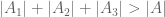
(For comparison, the parity problem predicts that one cannot hope to do any better than showing that  , so the above inequality is not ruled out by the parity problem obstruction.)
Then, just from the pigeonhole principle, one deduces the existence of ![n \in [N,2N]](https://s0.wp.com/latex.php?latex=n+%5Cin+%5BN%2C2N%5D&bg=ffffff&fg=545454&s=0&c=20201002) such that at least two of n, n+2, n+6 are prime, thus yielding a pair of primes whose gap is at most 6. This naive approach does not quite work directly, but by carefully optimising the argument (for instance, replacing the condition
such that at least two of n, n+2, n+6 are prime, thus yielding a pair of primes whose gap is at most 6. This naive approach does not quite work directly, but by carefully optimising the argument (for instance, replacing the condition  with something more like
 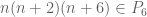 ), Goldston, Yildirim, and Pintz were able to show unconditionally that prime gaps in
 ![{}[N, 2N]](https://s0.wp.com/latex.php?latex=%7B%7D%5BN%2C+2N%5D&bg=ffffff&fg=545454&s=0&c=20201002) could be as small as
could be as small as  , and could in fact be as small as 16 infinitely often if one assumes the Elliot-Halberstam conjecture.
In a somewhat similar spirit, my result with Ben Green establishing that the primes contain arbitrarily long progressions proceeds by first using sieve theory methods to show that the almost primes (or more precisely, a suitable weight function  concentrated near the almost primes) are very pseudorandomly distributed, in the sense that several self-correlations of can be computed and agree closely with what one would have predicted if the almost primes were distributed randomly (after accounting for some irregularities caused by small moduli). Because of the parity problem, the primes themselves are not known to be as pseudorandomly distributed as the almost primes; however, the prime number theorem does at least tell us that the primes have a positive relative density in the almost primes. The main task is then to show that any set of positive relative density in a sufficiently pseudorandom set contains arithmetic progressions of any specified length; this combinatorial result (a “relative Szemerédi theorem“) plays roughly the same role that the pigeonhole principle did in the work of Goldston-Yildirim-Pintz. (On the other hand, the relative Szemerédi theorem works even for arbitrarily low density, whereas the pigeonhole principle does not; because of this, our sieve theory analysis is far less delicate than that in Goldston-Yildirim-Pintz.)
It is probably premature, with our current understanding, to try to find a systematic way to get around the parity problem in general, but it seems likely that we will be able to find some further ways to get around the parity problem in special cases, and perhaps once we have assembled enough of these special cases, it will become clearer what to do in general.
[Update, June 6: definition of almost prime modified, to specify that all prime factors are large. Reference to profinite integers deleted due to conflict with established notation.]


85 comments
Comments feed for this article
18 September, 2015 at 4:46 pm
The logarithmically averaged Chowla and Elliott conjectures for two-point correlations; the Erdos discrepancy problem | What's new
[…] such as (2) or (3) are known to be subject to the “parity problem” (discussed numerous times previously on this blog), which roughly speaking means that they cannot be proven solely […]
15 June, 2016 at 3:00 pm
Primos gemelos: Un vistazo a algunos resultados. – Lo fascinante de la teoría de números
[…] otra conjetura acerca de teoría de números bastante tratada. En palabras de Terence Tao, “Una especie de Hipotesis de Riemann super generalizada para […]
16 June, 2016 at 11:58 am
Anonymous
What is the best upper estimate for the number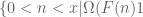 ? In the book Halberstam, Richert “Sieve_methods” only lower bounds. Could You recommend literature about upper bounds? Thanks.
16 June, 2016 at 12:15 pm
Anonymous
Sorry,
17 July, 2016 at 8:53 am
Notes on the Bombieri asymptotic sieve | What's new
[…] scalar thus embodies the “parity problem” for the twin prime conjecture (discussed in these previous blog […]
20 August, 2016 at 10:28 pm
Notes on the Bombieri asymptotic sieve - TAREA LISTA
[…] scalar thus embodies the “parity problem” for the twin prime conjecture (discussed in these previous blog […]
12 February, 2017 at 4:16 pm
Anonymous
Are there any known sieves of Twin Pairs that do not break down with an either/or at one of the numbers? — And if not, my main question is, Of all known sieves:
>> What is the farthest a sieve has gone when producing twin pairs before it breaks? <<
Lastly, if a sieve was found that never broke down, how could it be used to give a proof for the infinitude of twin pairs? ( I am lead to believe that even a perfect sieve is not a proof. Am I wrong?)
29 July, 2017 at 12:31 am
Mats Granvik
Is the use of eigenvalues allowed in approaching the parity problem?
https://oeis.org/A275345
20 September, 2017 at 9:37 am
Kyle Pratt
I apologize for posting a comment on an old post.
In your discussion of Selberg’s elementary proof of the PNT you mention that grows like
  . However, for every
  we have
  for some constant
  .
.
[Corrected, thanks – T.]
22 January, 2018 at 5:13 pm
Hammer and Nails | Radimentary
[…] Usually even the failure of certain techniques sheds light on shape of the difficulty. One classic example of an enlightening failure is the consistent overcounting (by exactly a factor of two!) of primes by sieve methods. This failure is so serious and unfixable that it has its own name: the Parity Problem. […]
25 February, 2018 at 7:48 am
DZ
The line “For comparison, the parity problem predicts that one cannot hope to do any better than showing that $|A_1|, |A_2|, |A_3| \geq |A|/2$ …” probably should be read $|A_1| + |A_2| +|A_3| \geq |A|/2$ ?
25 February, 2018 at 8:27 am
Terence Tao
Actually the statement is as I intended: it is possible to obtain a lower bound of the form through lower bounds on
  that are no stronger than
  ,
,  ,
,  . In contrast, one cannot prove a lower bound of the form
  in this fashion.
29 April, 2018 at 8:45 pm
Finding Coprime Pairs | Gödel's Lost Letter and P=NP
[…] comment by Ben Green neatly expresses the analytical motivation, as does section 4 of this paper. The […]
27 December, 2019 at 2:44 am
Fred Daniel Kline
I’m an amateur and in my attempts to find symmetry in Binary Goldbach, I had to make my odd number function use positive indexes. This eliminated a one-off issue for me. I don’t know how this would affect the Twin Prime parity.
2 August, 2021 at 5:34 am
Giovanni Di Savino
The only way to be sure of being able to find all the prime numbers is not, as mentioned in another post, to calculate but to understand the logic of the generation of prime numbers https://www.quora.com/How-come-la-distanza-tra-numeri-primi-soddisfa-la-versione-forte-della-congettura-di-Goldbach-Che-da-soluzione-alla-congettura-dei-gemelli/answer/Giovanni-163-1
19 April, 2022 at 4:20 pm
james
Is there a way to make the second display after (7) a bit more quantitively precise? For example if we sum the first display after (7) over as you suggested then we obtain
  . GRH then lets us conclude that
  . I agree this probably implies
  would not be of the correct order of magnitude (e.g.
  if we are counting primes) unless
  s are all very large and of the same sign or something. However, I don’t see how this rules out the possibility that e.g.
  which, although weak, would imply that there are infinitely many primes (or infinitely many twin primes in another setting). So to rephrase my question, is it possible to use you sketch argument to show that one shouldn’t expect even a very weak
  lower bound, i.e. I am not quite convinced by your conclusion that one shouldn’t expect to improve the trivial
  bound?
22 April, 2022 at 8:53 am
Terence Tao
Let’s adopt the (somewhat non-rigorous) Liouville pseudorandomness hypothesis for sake of discussion, so that behaves like a random sequence of +-1s. Then the sum
  is not only expected to be small in magnitude, but also to fluctuate in sign, and in particular be positive about 50% of the time, and so this wouuld force
  to be negative half the time, thus ruling out a uniform lower bound such as
  . Now it is true that this obstruction still does not rule out the possibility that one could maybe introduce a sieve that has a non-trivial, non-uniform bound that holds for infinitely many
  but not all
  , but this would be a very unusual species of sieve that does not resemble any existing sieve (which, if it works at all, would work for all sufficiently large
  , rather than for just a subset of
  ). Furthermore, such a sieve by its nature would have to be sensitive to the fluctuations of the Liouville function and so controlling such a sieve seems to be of comparable difficulty to the type of problem one is trying to attack in the first place.