
As you may already know, Danica McKellar, the actress and UCLA mathematics alumnus, has recently launched her book “Math Doesn’t Suck“, which is aimed at pre-teenage girls and is a friendly introduction to middle-school mathematics, such as the arithmetic of fractions. The book has received quite a bit of publicity, most of it rather favourable, and is selling quite well; at one point, it even made the Amazon top 20 bestseller list, which is a remarkable achievement for a mathematics book. (The current Amazon rank can be viewed in the product details of the Amazon page for this book.)
I’m very happy that the book is successful for a number of reasons. Firstly, I got to know Danica for a few months (she took my Introduction to Topology class way back in 1997, and in fact was the second-best student there; the class web page has long since disappeared, but you can at least see the midterm and final), and it is always very heartening to see a former student put her or his mathematical knowledge to good use :-) . Secondly, Danica is a wonderful role model and it seems that this book will encourage many school-age kids to give maths a chance. But the final reason is that the book is, in fact, rather good; the mathematical content is organised in a logical manner (for instance, it begins with prime factorisation, then covers least common multiples, then addition of fractions), well motivated, and interleaved with some entertaining, insightful, and slightly goofy digressions, anecdotes, and analogies. (To give one example: to motivate why dividing 6 by 1/2 should yield 12, she first discussed why 6 divided by 2 should give 3, by telling a story about having to serve lattes to a whole bunch of actors, where each actor demands two lattes each, but one could only carry the weight of six lattes at a time, so that only 

While I am not exactly in the target audience for this book, I can relate to its pedagogical approach. When I was a kid myself, one of my favourite maths books was a very obscure (and now completely out of print) book called “Creating Calculus“, which introduced the basics of single-variable calculus via concocting a number of slightly silly and rather contrived stories which always involved one or more ants. For instance, to illustrate the concept of a derivative, in one of these stories one of the ants kept walking up a mathematician’s shin while he was relaxing against a tree, but started slipping down at a point where the slope of the shin reached a certain threshold; this got the mathematician interested enough to compute that slope from first principles. The humour in the book was rather corny, involving for instance some truly awful puns, but it was perfect for me when I was 11: it inspired me to play with calculus, which is an important step towards improving one’s understanding of the subject beyond a superficial level. (Two other books in a similarly playful spirit, yet still full of genuine scientific substance, are “Darwin for beginners” and “Mr. Tompkins in paperback“, both of which I also enjoyed very much as a kid. They are of course no substitute for a serious textbook on these subjects, but they complement such treatments excellently.)
Anyway, Danica’s book has already been reviewed in several places, and there’s not much more I can add to what has been said elsewhere. I thought however that I could talk about another of Danica’s contributions to mathematics, namely her paper “Percolation and Gibbs states multiplicity for ferromagnetic Ashkin-Teller models on 
[Update, Aug 23: I added a non-technical “executive summary” of what the Chayes-McKellar-Winn theorem is at the very end of this post.]
— Statistical mechanics —
To begin the story, I would like to quickly review the theory of statistical mechanics. This is the theory which bridges the gap between the microscopic (particle physics) description of many-particle systems, and the macroscopic (thermodynamic) description, giving a semi-rigorous explanation of the empirical laws of the latter in terms of the fundamental laws of the former.
Statistical mechanics is a remarkably general theory for describing many-particle systems – for instance it treats classical and quantum systems in almost exactly the same way! But to simplify things I will just discuss a toy model of the microscopic dynamics of a many-particle system S – namely a finite Markov chain model. In this model, time is discrete, though the interval between discrete times should be thought of as extremely short. The state space is also discrete; at any given time, the number of possible microstates that the system S could be in is finite (though extremely large – typically, it is exponentially large in the number N of particles). One should view the state space of S as a directed graph with many vertices but relatively low degree. After each discrete time interval, the system may move from one microstate to an adjacent one on the graph, where the transition probability from one microstate to the next is independent of time, or on the past history of the system. We make the key assumption that the counting measure on microstates is invariant, or equivalently that the sum of all the transition probabilities that lead one away from a given microstate equals the sum of all the transition probabilities that lead one towards that microstate. (In classical systems, governed by Hamiltonian mechanics, the analogue of this assumption is Liouville’s theorem; in quantum systems, governed by Schrödinger’s equation, the analogue is the unitarity of the evolution operator.) We also make the mild assumption that the transition probability across any edge is positive.
If the graph of microstates was connected (i.e. one can get from any microstate to any other by some path along the graph), then after a sufficiently long period of time, the probability distribution of the microstates will converge towards normalised counting measure, as can be seen by basic Markov chain theory. However, if the system S is isolated (i.e. not interacting with the outside world), conservation laws intervene to disconnect the graph. In particular, if each microstate x had a total energy H(x), and one had a law of conservation of energy which meant that microstates could only transition to other microstates with the same energy, then the probability distribution could be trapped on a single energy surface, defined as the collection 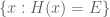
Physics has many conservation laws, of course, but to simplify things let us suppose that energy is the only conserved quantity of any significance (roughly speaking, this means that no other conservation law has a significant impact on the entropy of possible microstates). In fact, let us make the stronger assumption that the energy surface is connected; informally, this means that there are no “secret” conservation laws beyond the energy which could prevent the system evolving from one side of the energy surface to the other.
In that case, Markov chain theory lets one conclude that if the solution started out at a fixed total energy E, and the system S was isolated, then the limiting distribution of microstates would just be the uniform distribution on the energy surface
In practice, of course, a small system S is almost never truly isolated from the outside world S’, which is a far larger system; in particular, there will be additional transitions in the combined system 
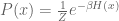
Now it would seem that in order to compute what this canonical ensemble is, one would have to know a lot about the external system S’, or the total energy E. Rather astonishingly, though, as long as S’ is much larger than S, and obeys some plausible physical assumptions, we can specify the canonical ensemble of S using only a single scalar parameter, the temperature T. To see this, recall in the microcanonical ensemble of 


Now it seems that it is hopeless to compute 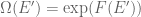


where 
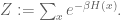
The canonical ensemble is thus specified completely except for a single parameter 

At the temperature extreme 


— Gibbs states —
One can of course continue developing the theory of statistical mechanics and relate temperature and energy to other macroscopic variables such as volume, particle number, and entropy (see for instance Schrödinger’s classic little book “Statistical thermodynamics“), but I’ll now turn to the topic of Gibbs states of infinite systems, which is one of the main concerns of the Chayes-McKellar-Winn paper.
A Gibbs state is simply a distribution of microstates of a system which is invariant under the dynamics of that system, physically, such states are supposed to represent an equilibrium state of the system. For systems S with finitely many degrees of freedom, the microcanonical and canonical systems given above are examples of Gibbs states. But now let us consider systems with infinitely many degrees of freedom, such as those arising from an infinite number of particles (e.g. particles in a lattice). One cannot now argue as before that the entire system is going to be in a canonical ensemble; indeed, as the total energy of the system is likely to be infinite, it is not even clear that such an ensemble still exists. However, one can still argue that any localised portion 

For systems with finitely many degrees of freedom, there is only one canonical ensemble at temperature T, and thus only one Gibbs state at that temperature. However, for systems with infinitely many degrees of freedom, it is possible to have more than one Gibbs state at a given temperature. This phenomenon manifests itself physically via phase transitions, the most familiar of which involves transitions between solid, liquid, and gaseous forms of matter, but also includes things like spontaneous magnetisation or demagnetisation. Closely related to this is the phenomenon of spontaneous symmetry breaking, in which the underlying system (and in particular, the energy functional H) enjoys some symmetry (e.g. translation symmetry or rotation symmetry), but the Gibbs states for that system do not. For instance, the laws of magnetism in a bar of iron are rotation symmetric, but there are some obviously non-rotation-symmetric Gibbs states, such as the magnetised state in which all the iron atoms have magnetic dipoles oriented with the north pole pointing in (say) the upward direction. [Of course, as the universe is finite, these systems do not truly have infinitely many degrees of freedom, but they do behave analogously to such systems in many ways.]
It is thus of interest to determine, for any given physical system, under what choices of parameters (such as the temperature T) one has non-uniqueness of Gibbs states. For “real-life” physical systems, this question is rather difficult to answer, so mathematicians have focused attention instead on some simpler toy models. One of the most popular of these is the Ising model, which is a simplified model for studying phenomena such as spontaneous magnetism. A slight generalisation of the Ising model is the Potts model; the Ashkin-Teller model, which is studied by Chayes-McKellar-Winn, is an interpolant betwen a certain Ising model and a certain Potts model.
— Ising, Potts, and Ashkin-Teller models —
All three of these models involve particles on the infinite two-dimensional lattice
As discussed earlier, in order to do statistical mechanics, we do not actually need to specify the exact mechanism by which the particles interact with each other; we only need to describe the total energy of the system. In these models, the energy is contained in the bonds between adjacent sites on the lattice (i.e. sites which are a unit distance apart). The energy of the whole system is then the sum of the energies of all the bonds, and the energy of each bond depends only on the state of the particles at the two endpoints of the bond. (The total energy of the infinite system is then a divergent sum, but this is not a concern since one only needs to be able to compute the energy of finite subsystems, in which one only considers those particles within, say, a square of length R.) The Ising, Potts, and Ashkin-Teller models then differ only in the number of states and the energy of various bond configurations. Up to some harmless normalisations, we can describe them as follows:
- In the classical Ising model, there are two magnetisation states (+1 and -1); the energy of a bond between two particles is -1/2 if they are in the same state, and +1/2 if they are in the opposite state (thus one expects the states to align at low temperatures and become non-aligned at high temperatures);
- In the four-state Ising model, there are four magnetisation states (+1,+1), (+1,-1), (-1,+1), and (-1,-1) (which can be viewed as four equally spaced vectors in the plane), and the energy of a bond between two particles is the sum of the classical Ising bond energy between the first component of the two particle states, and the classical Ising bond energy between the second component. Thus for instance the bond energy between particles in the same state is -1, particles in opposing states is +1, and particles in orthogonal states (e.g. (+1,+1) and (+1,-1)) is 0. This system is equivalent to two non-interacting classical Ising models, and so the four-state theory can be easily deduced from the two-state theory.
- In the degenerate Ising model, we have the same four magnetisation states, but now the bond energy between particles is +1 if they are in the same state or opposing state, and 0 if they are in an orthogonal state. This model essentially collapses to the two-state model after identifying (+1,+1) and (-1,-1) as a single state, and identifying (+1,-1) and (-1,+1) as a single state.
- In the four-state Potts model, we have the same four magnetisation states, but now the energy of a bond between two particles is -1 if they are in the same state and 0 otherwise.
- In the Ashkin-Teller model, we have the same four magnetisation states; the energy of a bond between two particles is -1 if they are in the same state, 0 if they are orthogonal, and
if they are in opposing states. The case
is the four-state Ising model, the case
is the Potts model, and the cases
are intermediate between the two, while the case
is the degenerate Ising model.
For the classical Ising model, there are two minimal-energy states: the state where all particles are magnetised at +1, and the state where all particles are magnetised at -1. (One can of course also take a probabilistic combination of these two states, but we may as well restrict attention to pure states here.) Since one expects the system to have near-minimal energy at low temperatures, we thus expect to have non-uniqueness of Gibbs states at low temperatures for the Ising model. Conversely, at sufficiently high temperatures the differences in bond energy should become increasingly irrelevant, and so one expects to have uniqueness of Gibbs states at high energy. (Nevertheless, there is an important duality relationship between the Ising model at low and high energies.)
Similar heuristic arguments apply for the other models discussed above, though for the degenerate Ising model there are many more minimal-energy states and so even at very low temperatures one only expects to obtain partial ordering rather than total ordering in the magnetisations.
For the Askhin-Teller models with 


This result is part of a very successful program, initiated by Fortuin and Kasteleyn, to analyse the statistical mechanics of site models such as the Ising, Potts, and Ashkin-Teller models via the random clusters generated by the bonds between these sites. (One of the fruits of this program, by the way, was the FKG correlation inequality, which asserts that any two monotone properties on a lattice are positively correlated. This inequality has since proven to be incredibly useful in probability, combinatorics and computer science.) The claims 

— Executive summary —
When one heats an iron bar magnet above a certain special temperature – the Curie temperature – the iron bar will cease to be magnetised; when one cools the bar again below this temperature, the bar can once again spontaneously magnetise in the presence of an external magnetic field. This phenomenon is still not perfectly understood; for instance, it is difficult to predict the Curie temperature precisely from the fundamental laws of physics, although one can at least prove that this temperature exists. However, Chayes, McKellar, and Winn have shown that for a certain simplified model for magnetism (known as the Ashkin-Teller model), the Curie temperature is equal to the critical temperature below which percolation can occur; this means that even when the bar is unmagnetised, enough of the iron atoms in the bar spin in the same direction that they can create a connected path from one end of the bar to another. Percolation in the Ashkin-Teller model is not fully understood either, but it is a simpler phenomenon to deal with than spontaneous magnetisation, and so this result represents an advance in our understanding of how the latter phenomenon works.
See also this explanation by John Baez.

60 comments
Comments feed for this article
12 August, 2016 at 9:01 am
Joe Kwiatkowski
I was a poor math student all through the K-12 experience, and looking back on it, it occurs to me that the most important factor conducive to being a good math student is discipline. One has to pay attention inn class (which I did not do) nd make a sincere attempt at the homework nightly (which I did not do). I did manage to pass all of my math courses, but it was only when I took a remedial course in intermediate algebra and trig, in technical college, that I took on a math course with proper discipline. The result was an A.
So the question becomes, does Ms. McKellar include in her book any suggestions as to how to motivate the student to deliver the effort necessary to do well in math? I would be interested to see her suggestions.
Side note there: I wonder how I rated against the rest of my peer group, motivation-wise. My hypothesis is, the most difficult job a parent has is to motivate his or her kids to generate proper effort in school. This cuts across races and sexes.
3 January, 2017 at 7:53 pm
Dhill114
The theme of Ms. McKellar’s childhood fictional drama series about learning or discovery seems to have transitioned nicely into reality for her adult life. Statistical mechanics is interesting but has many assumptions in practicality. I like the practical application of knowledge no matter who the audience is. Take it to the next level. For example a challenging concept probably just as relevant as the blog economic example or the concepts such as Pseudo-math applied Chayes-McKellar-which Winn seems to yield / correlate / implicate for the Energy or Heat transfer or Thermal effects on dipole or magnetic properties could be obscurely compared in a linear fashion to disruption of covalent bonds in molecules – research important for radioactive material compounds such as Tc-99m binding to pharmaceutical compounds or sodium iodide (I-131) valence +/- 1, may yield identification of high/low or Curie temperature or similar effects to render contaminated materials non-radioactive tangential to half life. If proven, in theory the relationship of heat or temperature effects to decontaminate or disassociate radioactive materials could allow for better adhesive filtration in applied science. Practical: incinerators used for disposal and disassociation and proper filtration of radioactive particulates and gas capture may be shown to be best practice vs. burial for disposal.
Math is just another language for communicating our understanding of things, just like the Internet of Things, whether truth or conjecture in real life. The abstract is growing in popularity. As a society we are constantly discovering what is already relational but hidden in plain sight.
17 August, 2017 at 5:32 am
Что такое огонь, и почему он жжёт — нанотехнологии.москва
[…] этого дано в блогпосте [28]Теренса Тао. Это […]
26 April, 2018 at 6:27 pm
Anonymous
Just for anyone still reading this, the link to the PDF for the “Chayes-McKellar-Winn theorem” is now here (the old link has died): http://www.danicamckellar.com/pdf/percolation.pdf
23 March, 2022 at 2:36 pm
What’s a fire and why does it burn? – A2Z Facts
[…] this is the Boltzmann distribution. For one possible justification of this, see this blog post by Terence Tao. This means that the probability […]
24 March, 2022 at 1:42 am
What’s a fire and why does it burn? (2016) by kvee - HackTech News
[…] constant); this is the Boltzmann distribution. For one possible justification of this, see this blog post by Terence Tao. This means that the probability […]