The classical foundations of probability theory (discussed for instance in this previous blog post) is founded on the notion of a probability space  – a space
  (the sample space) equipped with a
  -algebra
  (the event space), together with a countably additive probability measure
 ![{{\bf P}: {\cal E} \rightarrow [0,1]}](https://s0.wp.com/latex.php?latex=%7B%7B%5Cbf+P%7D%3A+%7B%5Ccal+E%7D+%5Crightarrow+%5B0%2C1%5D%7D&bg=ffffff&fg=000000&s=0&c=20201002) that assigns a real number in the interval
that assigns a real number in the interval ![{[0,1]}](https://s0.wp.com/latex.php?latex=%7B%5B0%2C1%5D%7D&bg=ffffff&fg=000000&s=0&c=20201002) to each event.
to each event.
One can generalise the concept of a probability space to a finitely additive probability space, in which the event space is now only a Boolean algebra rather than a -algebra, and the measure  is now only finitely additive instead of countably additive, thus
  when
when  are disjoint events. By giving up countable additivity, one loses a fair amount of measure and integration theory, and in particular the notion of the expectation of a random variable becomes problematic (unless the random variable takes only finitely many values). Nevertheless, one can still perform a fair amount of probability theory in this weaker setting.
In this post I would like to describe a further weakening of probability theory, which I will call qualitative probability theory, in which one does not assign a precise numerical probability value  to each event, but instead merely records whether this probability is zero, one, or something in between. Thus
  is now a function from to the set
  , where
  is a new symbol that replaces all the elements of the open interval
  . In this setting, one can no longer compute quantitative expressions, such as the mean or variance of a random variable; but one can still talk about whether an event holds almost surely, with positive probability, or with zero probability, and there are still usable notions of independence. (I will refer to classical probability theory as quantitative probability theory, to distinguish it from its qualitative counterpart.)
The main reason I want to introduce this weak notion of probability theory is that it becomes suited to talk about random variables living inside algebraic varieties, even if these varieties are defined over fields other than  or
or  . In algebraic geometry one often talks about a “generic” element of a variety
  defined over a field
  , which does not lie in any specified variety of lower dimension defined over . Once has positive dimension, such generic elements do not exist as classical, deterministic -points
  in , since of course any such point lies in the
  -dimensional subvariety
  of . There are of course several established ways to deal with this problem. One way (which one might call the “Weil” approach to generic points) is to extend the field to a sufficiently transcendental extension
  , in order to locate a sufficient number of generic points in
  . Another approach (which one might dub the “Zariski” approach to generic points) is to work scheme-theoretically, and interpret a generic point in as being associated to the zero ideal in the function ring of . However I want to discuss a third perspective, in which one interprets a generic point not as a deterministic object, but rather as a random variable
  taking values in , but which lies in any given lower-dimensional subvariety of with probability zero. This interpretation is intuitive, but difficult to implement in classical probability theory (except perhaps when considering varieties over or ) due to the lack of a natural probability measure to place on algebraic varieties; however it works just fine in qualitative probability theory. In particular, the algebraic geometry notion of being “generically true” can now be interpreted probabilistically as an assertion that something is “almost surely true”.
It turns out that just as qualitative random variables may be used to interpret the concept of a generic point, they can also be used to interpret the concept of a type in model theory; the type of a random variable is the set of all predicates  that are almost surely obeyed by . In contrast, model theorists often adopt a Weil-type approach to types, in which one works with deterministic representatives of a type, which often do not occur in the original structure of interest, but only in a sufficiently saturated extension of that structure (this is the analogue of working in a sufficiently transcendental extension of the base field). However, it seems that (in some cases at least) one can equivalently view types in terms of (qualitative) random variables on the original structure, avoiding the need to extend that structure. (Instead, one reserves the right to extend the sample space of one’s probability theory whenever necessary, as part of the “probabilistic way of thinking” discussed in this previous blog post.) We illustrate this below the fold with two related theorems that I will interpret through the probabilistic lens: the “group chunk theorem” of Weil (and later developed by Hrushovski), and the “group configuration theorem” of Zilber (and again later developed by Hrushovski). For sake of concreteness we will only consider these theorems in the theory of algebraically closed fields, although the results are quite general and can be applied to many other theories studied in model theory.
— 1. Qualitative probability theory – generalities —
We begin by setting up the foundations of qualitative probability theory, proceeding by close analogy with the more familiar quantitative probability theory (though of course we will have to jettison various quantitative concepts, such as mean and variance, from the theory).
As discussed in the introduction, we are replacing the unit interval by the three-element set  ; one could view this as the quotient space of in which the interior has been contracted to a single point . This space is still totally ordered:
  . The addition relation
  on contracts to an “addition” relation
  on , defined by the following rules:

with no other relations of the form in . Strictly speaking,  is not a binary operation here, as
  can evaluate to or to
  , but we keep the notation in order to emphasise the analogy with quantitative probability theory.
A qualitative probability space  is then a space
  equipped with a Boolean algebra
  (the measurable subsets of ) and a function
  with
with  , which is finitely additive in the sense that
  whenever
  are disjoint. It is easy to see that these measures are monotone (thus
  whenever
  ), and that
  . A measurable subset
  of is called a -null set if
  , and a -full set, a -conull set, or a -generic set if
  ; note that -full sets are the complements of -null sets and vice versa. A property
  of points
  is said to hold -almost everywhere or for -generic if it holds outside of a -null set (or equivalently, if it holds on a -generic set).
One can describe a qualitative probability measure on a Boolean space  purely through its null ideal
  of null sets, or equivalently through its full filter
  of full sets. Conversely, if a subset
  of is the full filter of some qualitative probability measure on if it obeys the following filter axioms:
- (Empty set)
 and
and  .
.
- (Monotonicity) If are in , and
 , then
  .
.
- (Intersection) If
 , then
  .
.
Furthermore is completely determined by the filter . Similarly for the null ideal (with suitably inverted axioms, of course). Thus, if one wished, one could replace the concept of a qualitative probability measure with the concept of an ideal or filter, but we retain the use of to emphasise the probabilistic interpretation of these objects.
One obvious way to create a qualitative probability measure is to start with a quantitative probability measure and “forget” the quantitative aspect of this measure by quotienting down to . Under some reasonable hypotheses, one can reverse this procedure and view many qualitative probability measures as quantitative probability measures to which this forgetful process has been applied. However, this reversal is usually not unique, and we will not try to use it here.
In quantitative probability theory, one can take two quantitative probability measures  on the same space and form an average
  for some
  , which is another quantitative probability measure. For instance, if is a probability measure and is a set with measure between and , then can be expressed as an average of the conditioned measures
  and
and  .
.
In analogy with this, we can take two qualitative measures on the same space and form the average  , defined by setting
  if and only if
  (or equivalently,
  if and only if
  ). If is a qualitative probability measure and is a set with measure , then we can form the conditioned measure
  , defined by setting
  if
if  (or equivalently
  if
if  ), and then one can check that is the average of the conditioned measures and
  .
.
We call a qualitative probability measure irreducible if it does not assign any set the intermediate measure of (or equivalently, the full filter is an ultrafilter); thus, irreducible qualitative probability measures are the same concept as finitely additive  -valued probability measures (which, as is well known, are essentially the same concept as ultrafilters). By the previous discussion, we see that a qualitative probability measure is irreducible if and only if it is not the average of two other measures.
In this paper we will primarily work with irreducible measures, but will occasionally have to deal with reducible measures, for instance when taking the conditional product (or pullback) of two irreducible measures over a third.
Given a measurable map  between two Boolean spaces
  ,
,  (thus the pre-image of any measurable set in
  by
by  is measurable in ), we can define the pushforward
  of any qualitative probability measure on to be the qualitative probability measure on defined by the usual formula
  . In particular, if embeds into , then any measure on can also be viewed as a measure on , which we call the extension of to .
We now discuss the issue of product measures in the qualitative setting. Here we will deviate a little from the usual probability formalism, in which one usually defines a product algebra  to be the minimal algebra that contains the Cartesian product of and
  . Here, it turns out to be more useful to have a more flexible (but not unique) notion of a product, in which more measurable sets are permitted. Namely, given two Boolean spaces , , we say that a Boolean space
  is a product of the two spaces if
  is the Cartesian product of and , and the following axioms are obeyed:
- (Products) If
 and
and  , then
  .
.
- (Slicing) If
 , then
  for all , and
  for all
  .
.
These axioms do not uniquely specify , but in practice each product space will have a canonical choice for attached to it.
Given two qualitative probability spaces  ,
,  , a qualitative probability space
  is a product of the two spaces if is a product of and , and the following assertions are equivalent for any :
-
 .
.
- For -almost every ,
 .
.
- For
 -almost every ,
  .
.
Of course, one could replace by here in the above equivalence, which can be thought of as a qualitative Fubini-Tonelli type theorem. Once one selects the product Boolean algebra , the product measure  is uniquely specified, if it exists at all; but (as in the setting of classical measure theory if one is not working with -finite measures), existence is not always automatic. (But in our applications, it will be.)
One can define products of more than two (but still finitely many) qualitative probability spaces in a similar fashion; we leave the details to the reader.
Now we are ready to set up qualitative probability theory. We need a qualitative probability space to serve as the sample space, event space, and probability measure. An event in is said to occur almost surely if it occurs on a -full set. Given an Boolean space  , a random variable is then a measurable map
  . We permit random variables that are only defined almost surely, thus is now a partial function defined on a -full event in ; as in quantitative probability theory or measure theory, we view random variables that agree almost surely as being essentially equivalent to each other. The law or distribution of is the pushforward
  of the qualitative probability measure; this is then a qualitative measure on . We say that two random variables
  agree in distribution, and write
  , if they have the same law.
Two random variables ,  are said to be independent if the distribution of the joint random variable
  is the product of the distributions of and
  separately. Here we need to specify a product Boolean algebra on the product space to make this definition well-defined, but in the applications we will consider, we will always have a canonical product algebra to select. One can define independence of more than two random variables in a similar fashion.
At the opposite extreme to independence, we say that a random variable  is determined by another random variable if there is a measurable map such that
  almost surely. The constrast between independence and determination (as well as a weaker property than determination we will consider later, namely algebraicity) will be the focus of the group chunk and group configuration theorems discussed in later sections.
As discussed in this previous blog post, in quantitative probability theory we often reserve the right to extend the underlying probability space , in order to introduce new sources of randomness, without destroying the probabilistic properties of existing random variables (such as their independence and determination properties). We say that an extension of a qualitative probability space is another qualitative probability space  together with a measurable map
  such that
  . One can then pull back any random variable to a random variable
  on the new probability space; by abuse of notation, we continue to refer to
  as . Probabilistic notions such as independence, law, or determination remain unchanged under such an extension.
— 2. Qualitative probability theory on definable sets —
For the purposes of this post, the qualitative probability measures we will care about will live in the theory of algebraically closed fields. We will assume some basic familiarity with algebraic geometry concepts, such as the dimension of a variety. The exact choice of field will not be important here, but one could work with the complex field  if desired (in which case one could (somewhat artificially) model the qualitative probability measures here by quantitative probability measures on complex varieties if one wished).
Henceforth is fixed; in contrast to usual model theory practice, we will not need to introduce some sufficiently large extension of to work in. The notion of measurability here will be given by the model-theoretic concept of definability. Namely, a definable set is a set  of the form

for some predicate that can be expressed in terms of the field operations  , a finite number of variables and constants in , the boolean symbols
  , the equality sign, the quantifiers
  (with all variables being quantified over ), and punctuation symbols (parentheses and colons). A definable map between two definable sets is a function whose graph
  is a definable set.
As is algebraically closed, the definable sets can be described quite simply. Define an irreducible quasiprojective variety, or variety for short, to be a Zariski-open dense subset of an irreducible affine variety over . One can show (using elimination of quantifiers in algebraically closed fields, the existence of which follows from Hilbert’s nullstellensatz) that a set is definable if and only if it is the union of a finite number of disjoint varieties.
We equip each definable set with the Boolean algebra  of definable subsets of ; this will be the only algebra we shall ever place on a definable set. Note that if
  are definable, then
  is a product space of
  and
and  as per the previous definition.
If is a qualitative probability measure on a definable set , the support of is defined to be the intersection of all the Zariski-closed sets of -full measure. As the Zariski topology is Noetherian, the support is always a closed set of full measure.
Remark 1 One can describe a qualitative probability measure through its type, defined as the set of all predicates which hold for -almost all . This concept is essentially the same as the concept of a type in model theory; the measure is irreducible if and only if the type is complete. In this post, we have essentially replaced the notion of a type with that of a qualitative probability measure, and so types will not appear explicitly in the rest of the post.
We now give some basic examples of qualitative probability measures on definable sets.
Example 1 If is a non-empty definable set of some dimension  (that is, is the largest dimension of all components of (or of its closure)), then the qualitative uniform probability measure
  on (or uniform measure, for short) is defined by setting all subsets of dimension
  or less to have measure zero, or equivalently all generic subsets of (that is, with finitely many sets of dimension removed) to have full measure. (Sets which contain a generic subset of some, but not all, of the -dimensional components of , then are assigned the intermediate measure.) The support of this measure is then the closure of the union of the -dimensional components. This measure is irreducible if and only if is almost irreducible in the sense that it only has one -dimensional component. Note that the algebraic geometry notion of genericity now coincides with the (qualitative) probabilistic notion of almost sureness: a (definable) property on holds generically if and only if it holds almost surely with respect to the uniform measure on .
If  are definable sets, then the uniform measure on is the product of the uniform measure on and the uniform measure on ; the proof of the Fubini-Tonelli type statement that justifies this may be found for instance in Lemma 13 of this paper of mine.
Example 2 If is almost irreducible and is a definable map, then the uniform measure on pushes forward to the uniform measure of some almost irreducible subset  of ; see e.g. Lemma A.8 of this previous paper of Breuillard, Green, and myself. Also, generic points in have fibres in of dimension
  , just as one would expect from naive dimension counting. If is not almost irreducible, the situation becomes a bit more complicated because the image on on different components of may have a different dimension, and so
  may become an average of uniform measures on sets of different dimension.
Exercise 1 Let be a qualitative probability measure on a definable set .
- (i) Show that is irreducible if and only if it is the uniform measure of some almost irreducible subset of .
- (ii) Show that is the average of finitely many uniform measures if and only if there does not exist a countable family of disjoint subsets of of positive measure. (Hint: greedily select disjoint varieties of of positive measure, starting with zero-dimensional varieties (points) and then increasing the dimension.)
We now use the formalism of qualitative probability theory from the previous section, but always working within the definable category; thus we require the sample space to also be a definable set, and that all random variables are required to be definable maps (or at least generically definable maps), which is a stronger condition than measurability.
— 3. The group chunk theorem —
Random variables can interact very nicely with groups  , if they come equipped with an appropriate invariant measure. To illustrate this, let us first return to the classical setting of quantitative probability theory, working exclusively with finite groups to avoid all measurability issues.
Given a finite group , let  be two elements of chosen uniformly and independently at random, and then form their product
  . This gives us a triple
  of random variables taking values in , which obey the following independence and determination properties:
- (i) (Uniform distribution) For any
 ,
,  has the uniform distribution on .
- (ii) (Independence) For any distinct
 ,
,  are independent.
- (iii) (Determination) For any distinct
 ,
,  is determined by .
- (iv) (Associativity) After extending the sample space as necessary, one can locate additional random variables
 taking values in such that
  (see figure), and such that any other triple
  for distinct
  which is not a permutation of the four triples already mentioned is jointly independent.
Indeed, to see the associativity axiom, let  be selected uniformly from independently of , and set
  and
and  . The associativity is depicted graphically in the figure below, in which three points connected by a line or curve indicate a dependence, but triples of points not joined by such a line or curve being independent.
In the converse direction, any triple on a finite set obeying the above axioms necessarily comes from an underlying group operation:
Proposition 1 (Probabilistic description of a finite group) Let be a finite non-empty set, and let  be random variables on that obey axioms (i)-(iv). Then there exists a group structure
  on such that
  .
.
Proof: By axiom (iii), we have for some binary operation  . From axiom (iv) we have

almost surely (and hence surely, as is finite); also from axioms (i), (iv) we see that  is uniformly distributed in
  . We conclude that the binary operation
  is associative, thus
  for all
  .
.
By axiom (iii), we see that for fixed  ,
,  is determined by
  and vice versa; from axioms (i), (ii), this implies that for fixed
  , the map
  is a bijection from to itself; similarly the map
  is a bijection from to itself. Note also from associativity that
  commutes with the right-action of in the sense that
  for all .
Conversely, given any bijection  that commutes with the right-action in the sense that
  for all
  , we claim that
  for a unique . Indeed, from axioms (i)-(iii), we know that is determined by
  , and so for any given
  , we may find such that
  . If this holds for a single
  , then it holds for all other by associativity, since
  commutes with the right action, and the map
  is a bijection. Thus we may identify with the space of bijections that commute with the right-action. This is clearly a group, and the property is then clear from construction.
Now that we see that a finite group, at least, may be described in terms of the probabilistic language of independence and determination. It is natural to ask whether similar results hold for infinite groups (with the slight modification that we now only expect to hold almost surely rather than surely, as we now will have non-trivial events of probability zero). Here we run into the technical difficulty that many groups – such as non-compact Lie groups, or algebraic groups defined over fields other than or – are not naturally equipped with a probability measure with which to define the concept of uniform distribution. However, if one is working in the definable category, one can use the language of qualitative probability theory instead and obtain the same result.
A definable group is a group which is a definable set, such that the group operations  and are definable maps. This notion is very close to, but subtly different from, that of the more commonly used notion of an algebraic group; the latter is a bit stricter because the group has to now be an algebraic variety, and the group operations have to be regular maps and not just definable maps. However, the two notions are quite close to each other, particularly in characteristic zero when they become equivalent up to definable group isomorphism, although additional subtleties arise in positive characteristic
  due to the existence of things like the inverse Frobenius automorphism
  , which is definable but not regular, and which can be used to definably “twist” an algebraic group. We will not discuss these issues further here, but see this survey of Bouscaren and this article of van den Dries for further discussion.
Theorem 2 (Group chunk theorem) Let be an almost irreducible definable set, and let be qualitative random variables taking values in , obeying axioms (i)-(iv). Then, after passing from to a generic subset, one may definably identify with a generic subset of an definable group  , so that
  almost surely. (To put it another way, there is a definable bijection
  between a generic subset of and a generic subset of , such that
  almost surely.)
This theorem is essentially due to Weil (although he worked instead in the category of algebraic varieties and algebraic groups, rather than definable sets and definable groups). It was extended to many other model-theoretic contexts (and in particular to stable theories) in the thesis of Hrushovski, although we will only focus on the classical algebraic geometry case here.
A typical example of a group chunk comes from taking a definable group and removing a lower dimensional subset of it, so that the group law is only generically defined (but this is still sufficient for defining  almost surely). For instance, one could let be the
  non-singular matrices
  , with (generically defined) group law given by matrix multiplication followed by projective normalisation to force the lower left coordinate to be (which is only defined if this coordinate does not vanish, of course). This can be viewed as an open dense subset of the projective special linear group
  , and the theorem is asserting that can be “completed” to this group, which can be interpreted as a definable group. ( can be viewed as an affine variety using, for instance, the adjoint representation. In any event, even projective varieties can be interpreted affinely in a definable fashion by the artificial device of breaking up the variety into finitely many pieces, which can be all fit into a sufficiently large affine space.)
We now prove Theorem 2. By axioms (i)-(iii), there is a generically defined, and definable, map such that almost surely. From axiom (iii) we then conclude the following cancellation axioms:
- (vii) (Left cancellation) For generic
 , there is a unique such that
  .
.
- (viii) (Right cancellation) For generic , there is a unique such that
 .
.
The associativity axiom then also gives  for generic
  .
.
These axioms also imply the following variants:
- (vii’) (Left cancellation) For generic
 , is the unique
  such that
  .
.
- (viii’) (Right cancellation) For generic , is the unique such that
 .
.
Indeed, from axiom (vii), we have a generically defined map  that maps a generic pair to
  , where is the unique
  such that . This map is generically injective; as
  is essentally irreducible, this map has to be generically bijective also, which gives (vii’), and (viii’) is proven similarly. (We call a partially defined map generically bijective if it can be made into a total bijection by refining to generic subsets.) We conclude that for generic
  , the maps
  and
and  are generically bijective.
To obtain a genuine group from rather than just a generic group, we perform a formal quotient construction, analogous to how the integers are formally constructed from the natural numbers (or the rationals from the integers). Define a formal pre-group element to be a definable subset  of with the following properties:
- (ix) (Vertical line test) For generic , there is exactly one
 such that
  .
.
- (ix’) (Vertical line test) For generic ,
 is the unique
  such that
  .
.
- (x) (Horizontal line test) For generic
 , there is exactly one
  such that .
- (x’) (Horizontal line test) For generic ,
 is the unique
  such that
  .
.
- (xi) (Translation invariance) For generic
 ,
,  lies in .
The axioms (ix)-(x’) are asserting that is a generic bijection. (Here and in the sequel we adopt the convention that a mathematical statement is automatically considered false if one or more of its terms are undefined; for instance,  is only true when
  and
and  is well-defined. Similarly, when using set-builder notation, we only include those elements in the set which are well-defined; for instance, in the set
  , is implicitly restricted to those values for which and are well-defined.)
Call two formal pre-group elements  are equivalent if they have a common generic subset, and then define a formal group element to be an equivalence class
 ![{[\Sigma]}](https://s0.wp.com/latex.php?latex=%7B%5B%5CSigma%5D%7D&bg=ffffff&fg=000000&s=0&c=20201002) of formal pre-group elements , and let be the space of formal group elements. At this point, we have to deal with the technical problem that is not obviously a definable set. However, observe that if is a formal pre-group element, then we have a definable generic bijection
of formal pre-group elements , and let be the space of formal group elements. At this point, we have to deal with the technical problem that is not obviously a definable set. However, observe that if is a formal pre-group element, then we have a definable generic bijection  from to , which makes essentially irreducible. If we then define
  to be the Zariski closure of the top dimensional component of (i.e. the support of the uniform measure on ), then is an irreducible closed variety, which depends only on the equivalence class of , with inequivalent pre-group elements giving distinct irreducible closed varieties. Finally, one can describe in terms of a generic element
  of , as being the closure of the top-dimensional component of
  , and generic elements produce such an objecft. As such, if we let be the set of all , then is in one-to-one correspondence with the space of formal group elements, and may be parameterised as a definable set using standard algebraic geometry tools (e.g. Chow coordinates, the Hilbert scheme, or elimination of imaginaries), as being the image under a generically definable map
  of with fibres of dimension
  . In particular, as is essentially irreducible with dimension
  , is essentially irreducible with dimension .
We define the identity element of to be the equivalence class of the diagonal  , and define the inverse of the equivalence class of a formal pre-group element to be the equivalence class of the reflection
  of . As for the group law, we use generic composition: given two formal pre-group elements , we define the composition
  to be the set of all pairs such that there exists for which is the unique element with
  , and is also the unique element with . One can check (somewhat tediously) that this descends to a well-defined operation on that gives it the structure of a definable group.
Next, for generic , the set  is a formal pre-group element, giving a generically defined map
  . One can verify that this map is generically definable, generically injective, and generically a homomorphism. The remaining task is to verify that has the same dimension as , as this together with essential irreducibility and generic injectivity gives generic bijectivity thanks to dimension counting. But for every formal pre-group element , we see that generic , there is a unique with , and furthermore that for generic ; in particular, is equivalent to
  and can thus be recovered from ; conversely, generic gives rise to a formal group element by this construction. This sets up a generically bijective map
  from
from  to , which shows that has the same dimension as , as required. This concludes the proof of Theorem 2.
— 4. The group configuration theorem —
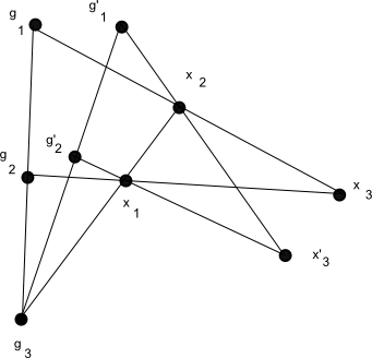
We now discuss a variant of the group chunk theorem that characterises group actions, known as the group configuration theorem. Again, to motivate matters we start with the quantitative probabilistic setting in the finite case. If is a finite group acting on a finite set , and are chosen independently and uniformly at random from , and  uniformly from (independently of ), and then one defines
  ,
,  ,and
,and  (or, more symmetrically, we have the constraints
  ,
,  ,
,  , and
, and  ), then we observe the following independence and determination axioms (setting
  and
and  for
for  ):
):
- (i’) (Uniform distribution) For any , has the uniform distribution on
 , and
, and  has the uniform distribution on
  .
.
- (ii’) (Independence) Any two of the random variables
 are independent.
- (iii’) (Determination) For any distinct , is determined by , and
 is determined by and
  .
.
- (v) (More independence) Any three of the random variables that are not of the form
 or
or  for distinct
  are independent.
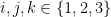
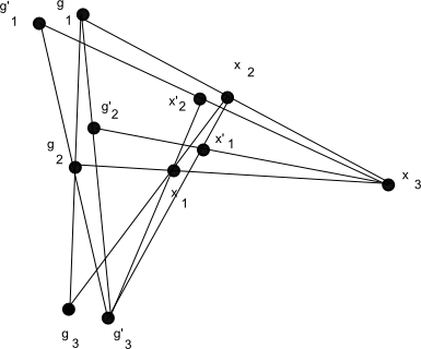
Axiom (ii’) is in fact a consequence of axiom (v), but we add it for emphasis. We refer to a sextet 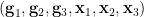 obeying the above axioms as a group configuration. It can be described graphically by the picture below, in which the collinearity of three random variables indicates a dependence between them, with non-collinear triples of variables being independent.

The group configuration theorem concerns a generalisation of the above situation, in which the determination properties in axiom (iii’) are relaxed to the weaker properties of algebraicity. (In additive combinatorics, this would correspond to moving from a “99%” situation in which algebraic structure is present almost everywhere, to a “1%” settng in which it is only present a positive fraction of the time.) We say that one random variable taking values in one definable set  is algebraic with respect to another random variable taking values in another definable set
  if there is a relation
  such that
  almost surely, and such that for each
  there are only finitely many
  such that
  . More informally, is algebraic over if determines up to a finite ambiguity. For instance, if is uniformly distributed in , then is algebraic with respect to any non-constant polynomial
  of
of  .
.
Two random variables are said to be interalgebraic if they are each algebraic over each other. For instance, if is uniformly distributed in the affine line , and  are two non-constant polynomials, then and
  are interalgebraic. Note that interalgebraicity is an equivalence relation.
Now we can give the group configuration theorem:
Theorem 3 (Group configuration theorem) Let  be almost irreducible definable sets, and let be random variables in respectively on a qualitative probability space obeying the following axioms:
- (i’) (Uniform distribution) For any , has the uniform distribution on , and has the uniform distribution on .
- (ii’) (Independence) Any two of the random variables are independent.
- (iii”) (Interalgebraicity) For any distinct , is algebraic over , and is algebraic over and .
- (v) (More independence) Any three of the random variables that are not of the form or for distinct are independent.
- (vi) (Irreducibility) The joint random variable has an irreducible distribution.
Then, after extending the (qualitative) probability space if necessary, there exist a definable group that acts definably on a definable space , as well as qualitative random variables  and
and  uniformly distributed in and respectively for , with algebraic over and interalgebraic with with , such that

almost surely, and with the  obeying the same independence and irreducibility hypotheses as the
  .
.
This theorem was first established by Zilber, who worked in the more general setting of strongly minimal theories, and then strengthened significantly in the thesis of Hrushovski, who treated the case of stable theories. (However, in these more general situations, the space is restricted to be “one-dimensional” for technical reasons.) We give a proof below the fold, following an exposition of Hrushovski’s method by Bouscaren. (See also a proof of a result very close to the above theorem, avoiding model-theoretic language, by Elekes and Szabo.) The irreducibility axiom (vi) can be relaxed, but then the conclusion becomes more complicated (there might not be a single group structure or group action involved, but rather an average of such actions).
The group configuration theorem has a number of applications to combinatorics; roughly speaking, this theorem is to “approximately associative” definable maps as Freiman’s theorem is for sets of small doubling. The aforementioned paper of Elekes and Szabo is one example of the configuration theorem in action; another is Theorem 41 of this paper of mine, which I proved by a different method (based on Riemann surface arguments), but for which a stronger statement has since been proven using the group configuration theorem by Hrushovski (private communication).
Now we prove Theorem 3. There are two main phases of the argument. The first phase involves upgrading several of the algebraicity hypotheses in axiom (iii”) to determination, by replacing several of the using algebraic changes of variable. Once this is done, the second phase consists of applying a modification of the proof of the group chunk theorem to locate the definable group (and also the definable space that acts on), and to connect this action to the group configuration.
We begin with a simple dimension counting observation. By the axioms, the random variable has an irreducible distribution and is thus uniformly distributed on some almost irreducible definable set , with algebraic over  , which is uniformly distributed on
  . Taking dimensions, we conclude that
  . Similarly for permutations. This implies that

for some natural number  ; a similar argument using the
  triples shows that

for some natural number  . Next, since
  are uniformly distributed on
  , and the other three variables
  are algebraic over these variables, we see that the tuple is uniformly distributed on some almost irreducible definable set of dimension
  .
.
We now begin the first phase. Currently, by axiom (iii”),  is algebraic over
  . We now use further dimension counting upgrade this algebraicity relationship to determination, basically by removing some information from .
Proposition 4 Let the assumptions be as in Theorem 3. Then there exists a random variable  which is interalgebraic with and uniformly distributed in some almost irreducible set
  , such that is determined by .
Proof: Let be the support of , and let  be the projection of onto
  , then is a closed variety, and as is algebraic over
  , is generically finite over . In particular, also has dimension
  . We then form the pullback (or base change)
  of two copies of over (a generic subset of) ; we view
  as a subset of
  . This is a definable set, but is not necessarily almost irreducible.
Now consider the projection  of to
of to  . The set contains the diagonal
  and thus has dimension at least . We claim that in fact has dimension exactly . Indeed, suppose this were not the case, then would contain an irreducible variety
  of dimension
  for some positive
  . Now observe that as is algebraic over , the projection of to
  is generically finite over
  , which has dimension
  ; taking pullback with itself, we conclude that the projection of to
  also has dimension . Thus, over a generic point in
  , the fibre of projected to has dimension at most
  . Similarly, the projection of this fibre to
  has dimension at most . Since is algebraic over
  , we conclude that the generic fibre of over a point in has total dimensino at most
  , so that the preimage of in has dimension at most

and is thus a lower-dimensional component of (or of after projecting to either of the two copies of ). Thus, if we pass to a suitable generic subset of , the projection of to has dimension . Passing to a further generic subset if necessary, we may assume that is algebraic in the sense that any horizontal or vertical line in meets in at most finitely many points. From the Noetherian property, we see that there is in fact a uniform upper bound  on how many such points can lie on a line (this is basically the degree of ).
We now define the random variable to be the set of all  with
with  , such that
  lies in the projection of (the generic portion of we are working with) to
  . By the above discussion, this is a finite subset of , and the set of all such possible
  can be parameterised in a definable way (indeed, it lies inside the
  -fold powers of over
  for
for  ), and is interalgebraic with . By construction, is also determined by
  ; as the latter is uniformly distributed on some almost irreducible set, is also, and the claim follows.
A similar argument provides a random variable  interalgebraic with
  such that
  is determined by
  . By replacing
  with
with  respectively, and checking that none of the axioms (i’). (ii’), (iii”), (v), (vi) are destroyed by this replacement, we see that we may reduce without loss of generality to the case in which we have the additional axiom
- (iii”‘) is determined by , and is determined by .
Now we turn to the task of making determined both by  and by
  . We are unable to effectively utilise (suitable permutations of) Proposition 4 here, because any replacement of by a random variable with less information content will likely destroy axiom (iii”‘). However, we can at least construct a random variable
  interalgebraic with that is determined by the joint random variable
  . Indeed, the support
  of
of  is generically finite over , and by repeating the dimension counting arguments from Proposition 4, we see tht the projection
  of the pullback
  to
to  has dimension at most , and so has finite fibres after passing to a generic subset. If we then set to be the fibre of over , we conclude as before that is interalgebraic with , and is clearly determined by . Also, each element of , together with , generically determines by axiom (iii”‘), and hence is determined by
  ; similarly is determined by . Thus by replacing with , we may impose the additional axiom
- (vii) is determined by

while retaining all previous axioms.
Now we perform the following “doubling” trick, creating some new random variables by extending the probability space. As before, let  be the support of . As
  is uniformly distributed in
  , we see that for generic
  and generic
  , there is a non-zero finite number of tuples
  such that
  . Similarly there are a non-zero finite number of tuples
  such that
  . Thus, for generic
  , if we let
  be the set of all tuples

such that

(see figure), then is a generically finite cover of (projecting onto the  coordinates). Thus, if we perform a base change of the probability space (which we view as lying over ) to , we may now create random variables

with the being an extension of the previous random variables of the same name.
Since is algebraic over  , we see (as is generic and deterministic) that
  is algebraic over . Similarly
  is algebraic over , and also
  is algebraic over and
  is algebraic over . From (iii) we also see that is determined by and , and is determined by and . Finally from (vii) we see that
  determine , and similarly
  determine . Thus if we set


then we see that
- is interalgebraic with for ;
- is interalgebraic with for ;
-
 is determined by
  ;
;
- is determined by
 ;
;
-
 is determined by
  ;
;
-
 is determined by
  .
.
Thus, by replacing and with and , we may now obtain the additional axiom
- (vii’) is determined by
 , and also is determined by
  .
.
We now have enough determination relations to begin the second phase of the argument, in which the arguments used to prove the group chunk theorem may be applied. Observe that  determine , and determine . Thus, for generic
  , we have a generically bijective definable map
  such that

almost surely, with  also depending definably on
  . Similarly, for generic
  , we have a generically bijective definable map
  such that

almost surely, with  also depending definably on
  .
.
We now relate the and to each other:
Lemma 5 After extending the probability space if necessary, there exist random variables  uniformly distributed in
  respectively, such that we almost surely have the identity
holds generically. Furthermore, any three of the  are independent, with the fourth being algebraic over these three.
Proof: Let  be the generic subset of consisting of those such that

(recall from our conventions that these statements implicitly require that all expressions be well-defined, thus for instance  must lie in the domain of
  for the second statement to be true). The set surjects onto a subset of
  of dimension
  (because is algebraic over
  , which is uniformly distributed over ), so the generic fibres have dimension
  . If we let
  , then
  thus has dimension
  . We view as a subset of
  and parameterise it as

By a base change, we may then find a set of random variables

uniformly distributed in , which restricts to the existing tuple of random variables.
By construction, one has

almost surely. On the other hand, the support of  has dimension at most
  (because
  are algebraic over
  ) and so for generic choices of these random variables, the set of possible
  has dimension at least
  ; since any one of these variables is algebraic over any other (once the are fixed), we conclude that cannot be restricted to any lower-dimensional set than . We conclude that almost surely, (2) holds generically.
The above discussion shows that the support of has dimension exactly ; as any three of are such that the remaining two random variables in are algebraic over these three, the final claims of the lemma follow.
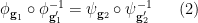
We rewrite (2) as
![\displaystyle [\phi_{{\bf g}_1}] \circ [\phi_{{\bf g}'_1}]^{-1} = [\psi_{{\bf g}_2}] \circ [\psi_{{\bf g}'_2}]^{-1} \ \ \ \ \ (4)](https://s0.wp.com/latex.php?latex=%5Cdisplaystyle++%5B%5Cphi_%7B%7B%5Cbf+g%7D_1%7D%5D+%5Ccirc+%5B%5Cphi_%7B%7B%5Cbf+g%7D%27_1%7D%5D%5E%7B-1%7D+%3D+%5B%5Cpsi_%7B%7B%5Cbf+g%7D_2%7D%5D+%5Ccirc+%5B%5Cpsi_%7B%7B%5Cbf+g%7D%27_2%7D%5D%5E%7B-1%7D+%5C+%5C+%5C+%5C+%5C+%284%29&bg=ffffff&fg=000000&s=0&c=20201002)
almost surely, where ![{[f]}](https://s0.wp.com/latex.php?latex=%7B%5Bf%5D%7D&bg=ffffff&fg=000000&s=0&c=20201002) is the equivalence class of a generically bijective, and definable, partial function up to generic equivalence, and inversion and composition on such equivalence classes is defined in the obvious manner. This equivalence class can be made definable by identifying with the closure of the top-dimensional component of the graph
is the equivalence class of a generically bijective, and definable, partial function up to generic equivalence, and inversion and composition on such equivalence classes is defined in the obvious manner. This equivalence class can be made definable by identifying with the closure of the top-dimensional component of the graph  of , and then expressing this in Chow coordinates (or using the Hilbert scheme); this makes equivalence classes
![\displaystyle \overline{{\bf g}}_1 := [\phi_{{\bf g}_1}]; \overline{{\bf g}}'_1 := [\phi_{{\bf g}'_1}]; \overline{{\bf g}}_2 := [\psi_{{\bf g}_2}]; \overline{{\bf g}}'_2 := [\psi_{{\bf g}'_2}]](https://s0.wp.com/latex.php?latex=%5Cdisplaystyle++%5Coverline%7B%7B%5Cbf+g%7D%7D_1+%3A%3D+%5B%5Cphi_%7B%7B%5Cbf+g%7D_1%7D%5D%3B+%5Coverline%7B%7B%5Cbf+g%7D%7D%27_1+%3A%3D+%5B%5Cphi_%7B%7B%5Cbf+g%7D%27_1%7D%5D%3B+%5Coverline%7B%7B%5Cbf+g%7D%7D_2+%3A%3D+%5B%5Cpsi_%7B%7B%5Cbf+g%7D_2%7D%5D%3B+%5Coverline%7B%7B%5Cbf+g%7D%7D%27_2+%3A%3D+%5B%5Cpsi_%7B%7B%5Cbf+g%7D%27_2%7D%5D&bg=ffffff&fg=000000&s=0&c=20201002)
into random variables uniformly distributed in some definable sets  , which are definable images of and thus almost irreducible (after passing to generic subsets of if necessary). We thus see that any three of
  are independent, and we have the relation

almost surely.
In particular, for fixed choices of  ,
,  ,
,  determines
  and vice versa. Thus
  and
and  have the same dimension, say
  . (This could be strictly less than , basically because the original sets
  may contain superfluous degrees of freedom which do not interact with the spaces
  .)
.)
We now let be the set of all equivalence classes of generically bijective and definable partial functions  with the following properties:
- For generic
 , there exists
  such that
 ![{[f] = \overline{g}_1 \circ (\overline{g}'_1)^{-1}}](https://s0.wp.com/latex.php?latex=%7B%5Bf%5D+%3D+%5Coverline%7Bg%7D_1+%5Ccirc+%28%5Coverline%7Bg%7D%27_1%29%5E%7B-1%7D%7D&bg=ffffff&fg=000000&s=0&c=20201002) .
.
- For generic , there exists such that .
- For generic
 , there exists
  such that
 ![{[f] = \overline{g}_2 \circ (\overline{g}'_2)^{-1}}](https://s0.wp.com/latex.php?latex=%7B%5Bf%5D+%3D+%5Coverline%7Bg%7D_2+%5Ccirc+%28%5Coverline%7Bg%7D%27_2%29%5E%7B-1%7D%7D&bg=ffffff&fg=000000&s=0&c=20201002) .
.
- For generic , there exists such that .
This is a definable set; is contained in the image of  by the map
  with fibres of dimension at most , and thus can have at most one component of dimension (and no larger dimensional components); on the other hand, from (5) contains the image of a generic subset of ; thus has dimension exactly and is essentially irreducible.
By construction, contains the (equivalence class of) the identity map on  and is closed under inversion. We also claim that it is closed under composition, which would make a definable group. Indeed, let
 ![{[f], [\tilde f] \in G}](https://s0.wp.com/latex.php?latex=%7B%5Bf%5D%2C+%5B%5Ctilde+f%5D+%5Cin+G%7D&bg=ffffff&fg=000000&s=0&c=20201002) . For generic , there exists such that . The map
. For generic , there exists such that . The map  is a generic bijection and is almost irreducible, and so
  is generic also. Thus, we may generically also find
  such that
 ![{[f'] = \overline{g}'_1 \circ (\overline{g}''_1)^{-1}}](https://s0.wp.com/latex.php?latex=%7B%5Bf%27%5D+%3D+%5Coverline%7Bg%7D%27_1+%5Ccirc+%28%5Coverline%7Bg%7D%27%27_1%29%5E%7B-1%7D%7D&bg=ffffff&fg=000000&s=0&c=20201002) , and hence
, and hence ![{[f] \circ [f'] = \overline{g}_1 \circ (\overline{g}''_1)^{-1}}](https://s0.wp.com/latex.php?latex=%7B%5Bf%5D+%5Ccirc+%5Bf%27%5D+%3D+%5Coverline%7Bg%7D_1+%5Ccirc+%28%5Coverline%7Bg%7D%27%27_1%29%5E%7B-1%7D%7D&bg=ffffff&fg=000000&s=0&c=20201002) . This gives the first property required for
. This gives the first property required for ![{[f] \circ [f']}](https://s0.wp.com/latex.php?latex=%7B%5Bf%5D+%5Ccirc+%5Bf%27%5D%7D&bg=ffffff&fg=000000&s=0&c=20201002) to lie in , and the other three are proven similarly.
to lie in , and the other three are proven similarly.
Having located the definable group , the next step is to locate a space that acts definably on. We first observe that generically acts on , by defining ![{[f] \cdot x_3 = x'_3}](https://s0.wp.com/latex.php?latex=%7B%5Bf%5D+%5Ccdot+x_3+%3D+x%27_3%7D&bg=ffffff&fg=000000&s=0&c=20201002) whenever
whenever  ,
,  , and
, and  is the unique element of such that (which, recall, is the closure of the top-dimensional component of the graph of ) contains
  . This is a definable, and generically defined operation which obeys the action axiom
  for generic
  .
.
To create a genuine action and not just a generic action, we perform yet another “quotient space construction” to extract a suitable space from as follows. Define a formal pre-point to be a definable subset of  obeying the following axioms:
- (xv) (Vertical line test) For generic , there is exactly one
 such that
  .
.
- (xv’) (Vertical line test) For generic , is the unique
 such that
  .
.
- (xvi) (Translation invariance) For generic
 , we have
  .
.
Two formal pre-points are equivalent if they have a common definable subset, and a formal point is an equivalence class of formal pre-points. We then let be the set of all formal points. If is a formal pre-point and  is a generic element of , then is equivalent to
  , and so is essentially irreducible; by similar arguments to before, we may now parameterise as a definable set, which is the image of the generically defined map
  described above with fibres of dimension at least and so has at most one component of dimension and no higher-dimensional components. The group acts on formal pre-points by the formula

one easily verifies that this is an action on formal pre-points which descends to a definable action on the space of formal points.
For generic  , the set
 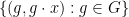 can be verified to be a formal pre-point; this gives a definable, generically defined map
  , which one can check to be generically injective; combined with the previous dimension control on , we now see that has dimension and is almost irreducible, with generically bijective. It can also be shown to generically preserve the action, in the sense that
  for generic
  .
.
Finally, we can set up the random variables and required for Theorem 3. We choose generic elements  , and then set
![\displaystyle \tilde {\bf g}_1 := [\phi_{{\bf g}_1}] \circ [\phi_{g_1^0}]^{-1}](https://s0.wp.com/latex.php?latex=%5Cdisplaystyle++%5Ctilde+%7B%5Cbf+g%7D_1+%3A%3D+%5B%5Cphi_%7B%7B%5Cbf+g%7D_1%7D%5D+%5Ccirc+%5B%5Cphi_%7Bg_1%5E0%7D%5D%5E%7B-1%7D&bg=ffffff&fg=000000&s=0&c=20201002)
![\displaystyle \tilde {\bf g}_2 := [\psi_{g_2^0}] \circ [\psi_{{\bf g}_2}]^{-1}](https://s0.wp.com/latex.php?latex=%5Cdisplaystyle++%5Ctilde+%7B%5Cbf+g%7D_2+%3A%3D+%5B%5Cpsi_%7Bg_2%5E0%7D%5D+%5Ccirc+%5B%5Cpsi_%7B%7B%5Cbf+g%7D_2%7D%5D%5E%7B-1%7D&bg=ffffff&fg=000000&s=0&c=20201002)
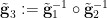

It is clear that for generic  , the are interalgebraic with , and that the relations (1) hold almost surely. Also, is clearly algebraic over for
  , and the are uniformly distributed in . For
  , we use the relation
  . As is algebraic over and ,
  is algebraic over and . Thus for generic , there can only be finitely many possible values of
  , giving the desired algebraicity.
We see that  is uniformly distributed in ; as
  almost surely, we conclude that is uniformly distributed over . The independence requirements on the now follow from the corresponding independence hypotheses on the .


6 comments
Comments feed for this article
16 November, 2013 at 11:05 pm
omar aboura
In the definition of “qualitative probability space” (third paragraph of Section 1), I think that the three must be
  .
.
[Corrected, thanks – T.]
17 November, 2013 at 12:13 am
Allen Knutson
PSL_2(k) isn’t projective; it’s the image of the adjoint representation of SL_2(k). More specifically it’s affine, being SO(the Killing form).
[Corrected, thanks – T.]
17 November, 2013 at 9:58 am
Rex
I believe “projective” here is just referring to the name of PSL and not asserting any projectivity.
[Allen was referring to an earlier version of the text, now corrected, in which there was some confusion in this regard – T.]
3 January, 2014 at 8:46 am
Sean Eberhard
An oft-used countably additive qualitative probability measure, completely unrelated to any genuine measure, is Baire category in a complete metric space. Say that if
if  is meagre and
  if
if  is comeagre.
9 May, 2021 at 10:18 am
Goursat and Furstenberg-Weiss type lemmas | What's new
[…] The ability to encode an abelian additive relation in terms of group-theoretic properties is vaguely reminiscent of the group configuration theorem. […]
13 May, 2021 at 4:48 pm
Goursat and Furstenberg-Weiss type lemmas – scroo0ooge
[…] The ability to encode an abelian additive relation in terms of group-theoretic properties is vaguely reminiscent of the group configuration theorem. […]