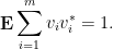
One of the basic tools in modern combinatorics is the probabilistic method, introduced by Erdos, in which a deterministic solution to a given problem is shown to exist by constructing a random candidate for a solution, and showing that this candidate solves all the requirements of the problem with positive probability. When the problem requires a real-valued statistic  to be suitably large or suitably small, the following trivial observation is often employed:
Proposition 1 (Comparison with mean) Let be a random real-valued variable, whose mean (or first moment)  is finite. Then

with positive probability, and

with positive probability.
This proposition is usually applied in conjunction with a computation of the first moment , in which case this version of the probabilistic method becomes an instance of the first moment method. (For comparison with other moment methods, such as the second moment method, exponential moment method, and zeroth moment method, see Chapter 1 of my book with Van Vu. For a general discussion of the probabilistic method, see the book by Alon and Spencer of the same name.)
As a typical example in random matrix theory, if one wanted to understand how small or how large the operator norm  of a random matrix
  could be, one might first try to compute the expected operator norm
  and then apply Proposition 1; see this previous blog post for examples of this strategy (and related strategies, based on comparing with more tractable expressions such as the moments
  ). (In this blog post, all matrices are complex-valued.)
Recently, in their proof of the Kadison-Singer conjecture (and also in their earlier paper on Ramanujan graphs), Marcus, Spielman, and Srivastava introduced an striking new variant of the first moment method, suited in particular for controlling the operator norm of a Hermitian positive semi-definite matrix . Such matrices have non-negative real eigenvalues, and so in this case is just the largest eigenvalue  of . Traditionally, one tries to control the eigenvalues through averaged statistics such as moments
  or Stieltjes transforms
  ; again, see this previous blog post. Here we use
  as short-hand for
  , where
  is the
  identity matrix. Marcus, Spielman, and Srivastava instead rely on the interpretation of the eigenvalues
  of as the roots of the characteristic polynomial
  of , thus

where  is the largest real root of a non-zero polynomial
  . (In our applications, we will only ever apply
  to polynomials that have at least one real root, but for sake of completeness let us set
  if has no real roots.)
Prior to the work of Marcus, Spielman, and Srivastava, I think it is safe to say that the conventional wisdom in random matrix theory was that the representation (1) of the operator norm was not particularly useful, due to the highly non-linear nature of both the characteristic polynomial map  and the maximum root map
  . (Although, as pointed out to me by Adam Marcus, some related ideas have occurred in graph theory rather than random matrix theory, for instance in the theory of the matching polynomial of a graph.) For instance, a fact as basic as the triangle inequality
  is extremely difficult to establish through (1). Nevertheless, it turns out that for certain special types of random matrices (particularly those in which a typical instance of this ensemble has a simple relationship to “adjacent” matrices in this ensemble), the polynomials
  enjoy an extremely rich structure (in particular, they lie in families of real stable polynomials, and hence enjoy good combinatorial interlacing properties) that can be surprisingly useful. In particular, Marcus, Spielman, and Srivastava established the following nonlinear variant of Proposition 1:
Proposition 2 (Comparison with mean) Let  . Let be a random matrix, which is the sum
  of independent Hermitian rank one matrices
  , each taking a finite number of values. Then

with positive probability, and

with positive probability.
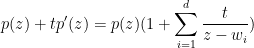
We prove this proposition below the fold. The hypothesis that each only takes finitely many values is technical and can likely be relaxed substantially, but we will not need to do so here. Despite the superficial similarity with Proposition 1, the proof of Proposition 2 is quite nonlinear; in particular, one needs the interlacing properties of real stable polynomials to proceed. Another key ingredient in the proof is the observation that while the determinant  of a matrix generally behaves in a nonlinear fashion on the underlying matrix , it becomes (affine-)linear when one considers rank one perturbations, and so depends in an affine-multilinear fashion on the
  . More precisely, we have the following deterministic formula, also proven below the fold:
Proposition 3 (Deterministic multilinearisation formula) Let be the sum of deterministic rank one matrices . Then we have
 \ \ \ \ \ (2)](https://s0.wp.com/latex.php?latex=%5Cdisplaystyle++p_A%28z%29+%3D+%5Cmu%5BA_1%2C%5Cldots%2CA_m%5D%28z%29+%5C+%5C+%5C+%5C+%5C+%282%29&bg=ffffff&fg=000000&s=0&c=20201002)
for all  , where the mixed characteristic polynomial
 }](https://s0.wp.com/latex.php?latex=%7B%5Cmu%5BA_1%2C%5Cldots%2CA_m%5D%28z%29%7D&bg=ffffff&fg=000000&s=0&c=20201002) of any matrices (not necessarily rank one) is given by the formula
of any matrices (not necessarily rank one) is given by the formula
 \ \ \ \ \ (3)](https://s0.wp.com/latex.php?latex=%5Cdisplaystyle++%5Cmu%5BA_1%2C%5Cldots%2CA_m%5D%28z%29+%5C+%5C+%5C+%5C+%5C+%283%29&bg=ffffff&fg=000000&s=0&c=20201002)
Among other things, this formula gives a useful representation of the mean characteristic polynomial  :
:
Corollary 4 (Random multilinearisation formula) Let be the sum of jointly independent rank one matrices . Then we have
 \ \ \ \ \ (4)](https://s0.wp.com/latex.php?latex=%5Cdisplaystyle++%5Cmathop%7B%5Cbf+E%7D+p_A%28z%29+%3D+%5Cmu%5B+%5Cmathop%7B%5Cbf+E%7D+A_1%2C+%5Cldots%2C+%5Cmathop%7B%5Cbf+E%7D+A_m+%5D%28z%29+%5C+%5C+%5C+%5C+%5C+%284%29&bg=ffffff&fg=000000&s=0&c=20201002)
for all  .
.
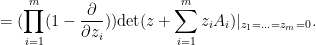
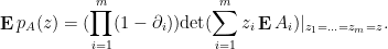
Proof: For fixed , the expression  is a polynomial combination of the
  , while the differential operator
  is a linear combination of differential operators
  for
for  . As a consequence, we may expand (3) as a linear combination of terms, each of which is a multilinear combination of
  for some . Taking expectations of both sides of (2) and using the joint independence of the , we obtain the claim.
In view of Proposition 2, we can now hope to control the operator norm of certain special types of random matrices (and specifically, the sum of independent Hermitian positive semi-definite rank one matrices) by first controlling the mean of the random characteristic polynomial . Pursuing this philosophy, Marcus, Spielman, and Srivastava establish the following result, which they then use to prove the Kadison-Singer conjecture:
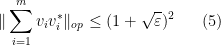
Theorem 5 (Marcus-Spielman-Srivastava theorem) Let . Let  be jointly independent random vectors in
  , with each
  taking a finite number of values. Suppose that we have the normalisation

where we are using the convention that  is the identity matrix whenever necessary. Suppose also that we have the smallness condition

for some  and all
  . Then one has
with positive probability.
Note that the upper bound in (5) must be at least (by taking to be deterministic) and also must be at least  (by taking the to always have magnitude at least
  ). Thus the bound in (5) is asymptotically tight both in the regime
  and in the regime
  ; the latter regime will be particularly useful for applications to Kadison-Singer. It should also be noted that if one uses more traditional random matrix theory methods (based on tools such as Proposition 1, as well as more sophisticated variants of these tools, such as the concentration of measure results of Rudelson and Ahlswede-Winter), one obtains a bound of
 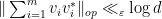 with high probability, which is insufficient for the application to the Kadison-Singer problem; see this article of Tropp. Thus, Theorem 5 obtains a sharper bound, at the cost of trading in “high probability” for “positive probability”.
In the paper of Marcus, Spielman and Srivastava, Theorem 5 is used to deduce a conjecture  of Weaver, which was already known to imply the Kadison-Singer conjecture; actually, a slight modification of their argument gives the paving conjecture of Kadison and Singer, from which the original Kadison-Singer conjecture may be readily deduced. We give these implications below the fold. (See also this survey article for some background on the Kadison-Singer problem.)
Let us now summarise how Theorem 5 is proven. In the spirit of semi-definite programming, we rephrase the above theorem in terms of the rank one Hermitian positive semi-definite matrices  :
:
Theorem 6 (Marcus-Spielman-Srivastava theorem again) Let be jointly independent random rank one Hermitian positive semi-definite matrices such that the sum  has mean

and such that

for some and all . Then one has
with positive probability.
In view of (1) and Proposition 2, this theorem follows from the following control on the mean characteristic polynomial:
Theorem 7 (Control of mean characteristic polynomial) Let be jointly independent random rank one Hermitian positive semi-definite matrices such that the sum has mean

and such that
for some and all . Then one has

This result is proven using the multilinearisation formula (Corollary 4) and some convexity properties of real stable polynomials; we give the proof below the fold.
Thanks to Adam Marcus, Assaf Naor and Sorin Popa for many useful explanations on various aspects of the Kadison-Singer problem.
— 1. Multilinearisation formula —
In this section we prove Proposition 3. The key observation is a standard one:
Lemma 8 (Determinant is linear with respect to rank one perturbations) Let  be matrices, with rank one. Then the polynomial
  is affine-linear (i.e. it is of the form
  for some coefficients
  ).
).
Proof: When  is the identity matrix, this follows from the Weinstein–Aronszajn identity
  , which shows in particular that
  for any rank one matrix
  . As the determinant is multiplicative, the claim then follows when is any invertible matrix; as the invertible matrices are dense in the space of all matrices, we conclude the general case of the lemma. (One can also prove this lemma via cofactor expansion, after changing variables to make
  or
or  a basis vector.)
Iterating this, we obtain
Corollary 9 (Determinant is multilinear with respect to rank one perturbations) Let  be matrices, with rank one. Then the polynomial
  is affine-multilinear, that is to say it is of the form
for some coefficients  .
.
Proof: By Lemma 8, the polynomial is affine-linear in each of the variables  separately (if one freezes the other
  variables
  ). The claim follows.
Now observe that if a one-variable polynomial  is affine-linear, then it can be recovered from its order Taylor expansion at the origin:

More generally, if a polynomial  is affine-multilinear in the sense of Corollary 9, then it can be recovered from an “order
  Taylor expansion” at the origin by the formula

Applying this to the polynomial in Corollary 9, we conclude that


Setting  and
and  , we obtain Proposition 3 as required.
— 2. Real stable polynomials and interlacing —
Now we prove Proposition 2. The key observation is that almost all of the polynomials one needs to work with here are of a special class, namely the real stable polynomials.
Definition 10 A polynomial  is stable if it has no zeroes in the region
  (in particular, is non-zero). A polynomial is real stable if it is stable and all of its coefficients are real.
Observe from conjugation symmetry that a real stable polynomial has no zeroes in either of the two regions and  . In particular, a one-variable real polynomial is stable if and only if it only has real zeroes. The notion of stability is however more complicated in higher dimensions. See this survey of Wagner for a more thorough discussion of the property of real stability.
To me, the property of being real stable is somewhat similar to properties such as log-convexity or total positivity; these are properties that are only obeyed by a minority of objects being studied, but in many key cases, these properties are available and can be very profitable to exploit. In practice, real stable polynomials get to enjoy the combined benefit of real analysis methods (e.g. the intermediate value theorem) with complex analysis methods (e.g. Rouche’s theorem), because of the guarantee that zeroes will be real.
A basic example of a real stable polynomial is the characteristic polynomial of a Hermitian matrix; this is a rephrasing of the fundamental fact that the eigenvalues of a Hermitian matrix are all real. There is a multidimensional version of this example, which will be the primary source of real stability for us:
Lemma 11 If are positive semi-definite Hermitian matrices, then the polynomial  is real stable.
Proof: It is clear that this polynomial is real (note that it takes real values for real inputs). To show that it is stable, observe that if  have positive imaginary part, then the skew-adjoint part of
  is strictly positive definite, and so is non-singular (since the quadratic form
  is non-degenerate).
Stable polynomials are also closed under restriction and under differential operators such as  .
.
Lemma 12 Let  be a real stable polynomial of
  variables.
- (Restriction) If
 and
and  is real, then the polynomial
  is a real stable polynomial of variables, unless it is identically zero.
- (Differentiation) For any real , the polynomial
 is a real stable polynomial of variables.
Similarly for permutations of the variables.
Proof: The final claim is clear, as the property of real stability is unchanged under permutation of the variables.
We first prove the restriction claim. The polynomial is clearly real. If we have a zero  with
with  having positive imaginary part, but
  does not vanish identically, then by the stable nature of zeroes (see, e.g., Rouche’s theorem) we will also have a nearby zero
  for any
  sufficiently close to , with
  arbitrarily close to
  . In particular, by setting have positive imaginary part, we contradict the stability of
  .
.
Now we turn to the differentiation claim. Again the real nature of is clear. To prove stability, it suffices after freezing the first variables to show that  is stable whenever
  is stable. We may of course take non-zero. But a stable polynomial of one variable may be factored as
  for some roots
  with non-positive imaginary part. Since
we see that if has positive imaginary part, then the imaginary part of  has the opposite sign to , and is in particular non-zero; since has no zeroes in the upper half-plane, neither does .
Combining these facts with (3), we immediately obtain:
Corollary 13 (Mixed characteristic polynomials are real stable) If are positive semi-definite matrices, then ![{\mu[A_1,\ldots,A_m]}](https://s0.wp.com/latex.php?latex=%7B%5Cmu%5BA_1%2C%5Cldots%2CA_m%5D%7D&bg=ffffff&fg=000000&s=0&c=20201002) is real stable. In other words, all the zeroes of are real.
is real stable. In other words, all the zeroes of are real.
Now, we relate stability with “convexity” properties of the largest root. Note in general that if  is a convex combination of two polynomials
  , that there is no requirement that
  lie between and
  . For instance, if
  and
and 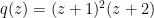 , then
  and
and  , but
, but 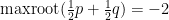 . Note also that are stable in this case. However the situation improves when one also assumes that all convex combinations of are stable:
Lemma 14 (Comparison with mean) Let  be real stable polynomials of one variable that are monic of the same degree. Suppose that
  is also real stable for every
  . Then for every
  ,
, 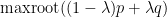 lies between and .
Proof: We may of course assume  . Without loss of generality let us assume
  , so our task is to show that

The second inequality is easy: as are monic,  is positive for
  and
and  is positive for
  , and so
  is positive for
  , giving the claim.
The first inequality is trickier. Suppose it fails; then  has no zero in
 ![{[\hbox{maxroot}(p), \hbox{maxroot}(q)]}](https://s0.wp.com/latex.php?latex=%7B%5B%5Chbox%7Bmaxroot%7D%28p%29%2C+%5Chbox%7Bmaxroot%7D%28q%29%5D%7D&bg=ffffff&fg=000000&s=0&c=20201002) . We have already seen that this polynomial is positive at , thus it must also be positive at . In other words,
. We have already seen that this polynomial is positive at , thus it must also be positive at . In other words,  is positive at . Since already had a zero at and was positive to the right of this zero, we conclude that has at least two zeroes (counting multiplicity) to right of . On the other hand, for sufficiently close to
  ,
,  has no zeroes to the right of , and all intermediate convex combinations
  cannot vanish at . Thus, at some intermediate value of , the number of real zeroes of to the right of must acquire a jump discontinuity (e.g. two real zeroes colliding and then disappearing, or vice versa), but this contradicts Rouche’s theorem and real stability.
One can control other roots than the maximal roots of  by these arguments, and show that these polynomials have a common interlacing polynomial of one lower degree, but we will not need these stronger results here.
Specialising this to mixed characteristic polynomials (which are always monic of degree  ), we conclude
Corollary 15 (Comparison with mean) Let be jointly independent random rank one positive semi-definite Hermitian matrices, with each taking finitely many values. For any  and any fixed choice of
  , we have
![\displaystyle \hbox{maxroot}( \mu[ A_1,\ldots,A_{j-1},A_j,\mathop{\bf E} A_{j+1},\ldots,\mathop{\bf E} A_m] )](https://s0.wp.com/latex.php?latex=%5Cdisplaystyle++%5Chbox%7Bmaxroot%7D%28+%5Cmu%5B+A_1%2C%5Cldots%2CA_%7Bj-1%7D%2CA_j%2C%5Cmathop%7B%5Cbf+E%7D+A_%7Bj%2B1%7D%2C%5Cldots%2C%5Cmathop%7B%5Cbf+E%7D+A_m%5D+%29+&bg=ffffff&fg=000000&s=0&c=20201002)
![\displaystyle \leq \hbox{maxroot}( \mu[ A_1,\ldots,A_{j-1}, \mathop{\bf E} A_j,\mathop{\bf E} A_{j+1},\ldots,\mathop{\bf E} A_m] )](https://s0.wp.com/latex.php?latex=%5Cdisplaystyle+%5Cleq+%5Chbox%7Bmaxroot%7D%28+%5Cmu%5B+A_1%2C%5Cldots%2CA_%7Bj-1%7D%2C+%5Cmathop%7B%5Cbf+E%7D+A_j%2C%5Cmathop%7B%5Cbf+E%7D+A_%7Bj%2B1%7D%2C%5Cldots%2C%5Cmathop%7B%5Cbf+E%7D+A_m%5D+%29&bg=ffffff&fg=000000&s=0&c=20201002)
with positive probability, and
![\displaystyle \geq \hbox{maxroot}( \mu[ A_1,\ldots,A_{j-1}, \mathop{\bf E} A_j,\mathop{\bf E} A_{j+1},\ldots,\mathop{\bf E} A_m] )](https://s0.wp.com/latex.php?latex=%5Cdisplaystyle+%5Cgeq+%5Chbox%7Bmaxroot%7D%28+%5Cmu%5B+A_1%2C%5Cldots%2CA_%7Bj-1%7D%2C+%5Cmathop%7B%5Cbf+E%7D+A_j%2C%5Cmathop%7B%5Cbf+E%7D+A_%7Bj%2B1%7D%2C%5Cldots%2C%5Cmathop%7B%5Cbf+E%7D+A_m%5D+%29&bg=ffffff&fg=000000&s=0&c=20201002)
with positive probability.
Proof: For fixed ,  is a convex combination of all the values of
  that occur with positive probability, and hence (by the affine-multilinear nature of
  )
) ![{\mu[ A_1,\ldots,A_{j-1}, \mathop{\bf E} A_j,\mathop{\bf E} A_{j+1},\ldots,\mathop{\bf E} A_m]}](https://s0.wp.com/latex.php?latex=%7B%5Cmu%5B+A_1%2C%5Cldots%2CA_%7Bj-1%7D%2C+%5Cmathop%7B%5Cbf+E%7D+A_j%2C%5Cmathop%7B%5Cbf+E%7D+A_%7Bj%2B1%7D%2C%5Cldots%2C%5Cmathop%7B%5Cbf+E%7D+A_m%5D%7D&bg=ffffff&fg=000000&s=0&c=20201002) is a convex combination of the
is a convex combination of the ![{\mu[ A_1,\ldots,A_{j-1}, A_j,\mathop{\bf E} A_{j+1},\ldots,\mathop{\bf E} A_m]}](https://s0.wp.com/latex.php?latex=%7B%5Cmu%5B+A_1%2C%5Cldots%2CA_%7Bj-1%7D%2C+A_j%2C%5Cmathop%7B%5Cbf+E%7D+A_%7Bj%2B1%7D%2C%5Cldots%2C%5Cmathop%7B%5Cbf+E%7D+A_m%5D%7D&bg=ffffff&fg=000000&s=0&c=20201002) over the same range of . On the other hand, by Corollary 13, all such convex combinations are real stable. Iterating Lemma 14, we see that
over the same range of . On the other hand, by Corollary 13, all such convex combinations are real stable. Iterating Lemma 14, we see that ![{\hbox{maxroot}(\mu[ A_1,\ldots,A_{j-1}, \mathop{\bf E} A_j,\mathop{\bf E} A_{j+1},\ldots,\mathop{\bf E} A_m])}](https://s0.wp.com/latex.php?latex=%7B%5Chbox%7Bmaxroot%7D%28%5Cmu%5B+A_1%2C%5Cldots%2CA_%7Bj-1%7D%2C+%5Cmathop%7B%5Cbf+E%7D+A_j%2C%5Cmathop%7B%5Cbf+E%7D+A_%7Bj%2B1%7D%2C%5Cldots%2C%5Cmathop%7B%5Cbf+E%7D+A_m%5D%29%7D&bg=ffffff&fg=000000&s=0&c=20201002) must lie in the convex hull of the
must lie in the convex hull of the ![{\hbox{maxroot}(\mu[ A_1,\ldots,A_{j-1}, A_j,\mathop{\bf E} A_{j+1},\ldots,\mathop{\bf E} A_m])}](https://s0.wp.com/latex.php?latex=%7B%5Chbox%7Bmaxroot%7D%28%5Cmu%5B+A_1%2C%5Cldots%2CA_%7Bj-1%7D%2C+A_j%2C%5Cmathop%7B%5Cbf+E%7D+A_%7Bj%2B1%7D%2C%5Cldots%2C%5Cmathop%7B%5Cbf+E%7D+A_m%5D%29%7D&bg=ffffff&fg=000000&s=0&c=20201002) , and the claim follows.
, and the claim follows.
Iterating the above corollary for  and using Proposition 3, we obtain Proposition 2 as desired.
— 3. Convexity —
In order to establish Theorem 7, we will need some convexity properties of real stable polynomials , or more precisely of the log-derivatives  of such polynomials, when one is “above” all the zeroes. We begin with the one-dimensional case:
Lemma 16 (One-dimensional convexity) Let be a real stable polynomial of one variable, and let  be the logarithmic derivative (which is defined away from the zeroes of ). Then
 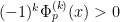 whenever
  and
and  . In particular,
  is positive, decreasing, and strictly convex to the right of .
Proof: If we factor  , where
  are the real roots, then
 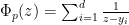 . From direct computation we have
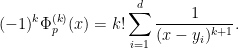
Since  is positive when , the claim follows.
Now we obtain a higher dimensional version of this lemma. If is a real stable polynomial, we say that a point  lies above the roots of if has no zeroes on the orthant
  .
.
Lemma 17 (Multi-dimensional convexity) Let be a real stable polynomial of variables, let  , and let
  be the logarithmic derivative in the
  direction. Then
  whenever
  and
and  lies above the roots of . In particular, the function
  is non-negative, non-increasing, and convex for non-negative .
Proof: For  or
or  , the claim follows from Lemma 16 after freezing all the other variables, so we may assume that
  and
and  . By freezing all the other variables and relabeling, we may assume that
  ,
,  , and
, and  , thus
  is a real stable polynomial,
  lies above the roots of , and the task is to show that
for all  . Using the variables
  to denote differentiation instead of
  , the left-hand side is equal to

so it suffices to show that  is non-decreasing in the
  direction. By continuity, it suffices to do this for generic (thus, we may exclude a finite number of exceptional if we wish).
For fixed , the polynomial  is real stable, and thus has real roots, which we denote as
  (counting multiplicity). For generic , the number of roots does not depend on , the
  can be chosen to vary smoothly in , and the multiplicity of each root is locally constant in (the latter claim can be seen by noting that the roots of
  of multiplicity at least
  are the same as the roots of the resultant of polynomial and its first
  derivatives
 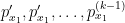 , and the set of the latter roots are generically smoothly varying in ). We then have

so it suffices to show that each of the  is a non-increasing function of . But if
  lies above the roots of , then the all lie below
  ; so it suffices to show that the are all generically non-increasing. But if this were not the case, then (as is generically smooth), would have a positive derivative for all in an open interval. In particular, there is an
  such that the root has positive derivative and a constant multiplicity for all sufficiently close to . This root depends analytically on near (this can be seen by noting that is the unique and simple root near
  of the
  derivative of and using the inverse function theorem), so by analytic continuation we conclude that for complex
  near , the polynomial
  has a complex root
  near that depends complex analytically on . Since the derivative of
  at is a positive real, we conclude that there are zeroes
  of near
  with
with  both strictly positive, contradicting stability, and the claim follows.
Now we begin the proof of Theorem 7. We abbreviate  as
as  . We start with Proposition 3 to write
From the hypothesis  , we may rewrite
and so after translating the by , we have
Replacing each by their mean, we reduce to showing the following deterministic estimate:
Theorem 18 Let be Hermitian positive semi-definite matrices such that
and such that
for some and all . Let be the polynomial
Then  lies above the roots of
  .
.
We will prove this theorem as follows. First observe that  lies above the roots of for any
  , since
  is positive semi-definite whenever
  , and so
  is non-singular in this region. We now wish to pass from to by successive application of the derivative operators
  . An initial step in this direction is the following elementary consequence of the monotonicity properties from Lemma 17.
Lemma 19 Let  be a real stable polynomial, and suppose that
  lies above the roots of . Suppose that
  , with the stability bound

Then also lies above the roots of  .
.
Proof: By the monotonicity properties in Lemma 17,  for all
  above (by which we mean that
  for all ). On the other hand, as
  is non-zero in this region,
  can only vanish when
  is equal to , and so lies above the roots of as claimed.
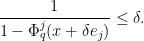
Unfortunately, this lemma does not directly lend itself to iteration, because the lemma provides no control on  . To fix this problem, we need the following more complicated variant of Lemma 19:
Lemma 20 Let be a real stable polynomial, and suppose that lies above the roots of . Suppose that , with the stability bound
for some  . Then
  lies above the roots of
  , and furthermore one has the monotonicity
for all  .
.
Proof: From Lemma 19 we already know that lies above the roots of , and so does also. Now we prove (9). Above the roots of , we factorise

and thus

Applying , we conclude that

The claim (9) is then equivalent to

On the other hand, by Lemma 17,  is convex for
  , and thus

But

and this quantity is non-positive at thanks to Lemma 17. Thus it suffices to show that
But by Lemma 17 and (8) one has
and the claim follows.
We can iterate this to obtain
Corollary 21 Let be a real stable polynomial, and suppose that lies above the roots of . Suppose that

for some and all . Then  lies above the roots of
  .
.
Proof: For each  , set
, set  and
and  . By Lemma 20 induction we see that for each ,
  lies above the roots of
  with
with

for all . Setting  , we obtain the claim.
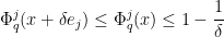
Finally, we prove Theorem 18. By definition, we have

and hence on taking  and using the Jacobi formula we conclude that

In particular, for any , we may use (6), (7) to conclude that
As remarked before, lies above the zeroes of . Thus, if we choose  such that
then by Corollary 21, we conclude that  lies above the zeroes of . To optimise
  subject to the constraint (11), we set
  and
and  , and Theorem 18 follows.
— 4. Weaver, Akemann-Anderson, and paving —
Theorem 5 is probabilistic in nature, but by specialising to a specific type of random vector (and by taking advantage of the freedom to enlarge the vector space  , since the bounds are independent of the dimension ), we obtain the following deterministic consequence:
Theorem 22 (Weaver-type bound) Let  be integers and
  be real numbers. Suppose that
  are such that
  for all
  and
and
for every unit vector  (i.e.,
  is a –tight frame), then there exists a partition
  into
into  components such that
for  and every unit vector
  .
.
Proof: Let notation and the hypotheses be as in the theorem. Define the independent random vectors  in the
  -dimensional tensor product
  of and
  by setting
for each , where  are sampled uniformly and independently from
  . From (12) one has

so a brief calculation shows that
(Here is the identity transformation on .) Also, we have

for all . Applying Theorem 5, we conclude that

with positive probability. In particular, this occurs for at least one realisation of the . Setting  to be those for which
  for each , we conclude that
for  ; testing this against a unit vector we conclude that

and the claim follows after a little arithmetic.
For a given  , the Weaver conjecture
  asserts for
  the existence of a such that the above theorem holds with the upper bound in (13) replaced by
  for some absolute constant
  . This is easily seen to follow from (13) by taking large enough. For instance (as noted by Marcus, Spielman, and Srivastava), if one takes
  then the upper bound in (13) is
  , giving the case of Weaver’s conjecture, which was already known to imply the Kadison-Singer conjecture (see e.g. this paper of Bice for an ultrafilter-based proof of this fact). Note also that in the large limit (keeping fixed), the bound in (13) approaches , which is the optimal value (as can be seen by considering the case where each has the maximal magnitude of
  ); this will be important later.
We can dualise Theorem 22 as follows, giving a bound of Akemann-Anderson type:
Corollary 23 (Paving conjecture for projections) Let  , and let
  be an
be an  orthogonal projection matrix, that is to say an idempotent Hermitian matrix. Suppose that we have the bound
  for all
  and some . Then, for any
  , there exists a partition
  of the identity into diagonal projections
  (i.e. the are diagonal matrices with s and s on the diagonal, that sum to the identity matrix) such that

for all .
Proof: Let  be the range of
  , then
  are vectors in with

Also, for any unit vector  , we have


Applying Theorem 22 with  ,
,  ,
,  , we can find a partition such that
for all unit vectors and . If we let  be the diagonal projection
  , then

and so

for all in . Thus

and thus on squaring

as desired.
This is a special case of the Kadison-Singer paving conjecture, but we may use a number of standard maneuvers to amplify this to the full paving conjecture, loosely following the papers of Popa and of Akemann-Weaver. First, by using the “dilation trick“, we may relax the hypothesis of being a projection:
Corollary 24 (Paving conjecture for positive semi-definite matrices) Let , and let be a Hermitian positive semi-definite matrix with the bound  for some
  . Suppose that we have the bound for all and some . Then, for any , there exists a partition of the identity into diagonal projections such that

for all .
Proof: By scaling we may set . The matrix is no longer a projection matrix, but by the spectral theorem and the hypotheses on , we still have a decomposition of the form
where  are an orthonormal basis for , and
  for all .
Now we embed in  for some large
  . If is large enough (depending on
  ), we may find orthonormal vectors
  with disjoint supports, such that each of the
  have coefficients of magnitude at most
  . We may then form the dilated vectors
which are an orthonormal system in , and the dilated operator

which is an orthogonal projection on . This can be viewed as a  matrix, whose top left minor is . By construction, all the diagonal entries of this matrix are at most . Applying Corollary 23, we may find a partition
  of the identity matrix on into diagonal projections
  such that

for all . If we let be the component of  that maps to (i.e. the top left minor), then the are diagonal matrices summing to the identity, and we have

for all , as required.
Now we shift by a multiple of the identity:
Corollary 25 (One-sided paving for Hermitian matrices) Let , and let be a Hermitian matrix with vanishing diagonal, whose eigenvalues lie between  and for some . Then, for any , there exists a partition of the identity into diagonal projections such that for each
  , the eigenvalues of
  lie between and
  .
.
Proof: Apply Corollary 24 with replaced by  , replaced by
  , and set equal to .
We combine this result with its reflection:
Corollary 26 (Paving conjecture for Hermitian matrices) Let , and let be a Hermitian matrix with vanishing diagonal, with for some . Then, for any , there exists a partition 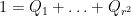 of the identity into diagonal projections
  such that

for all  .
.
Proof: The eigenvalues of lie between and . By Corollary 25, we may find a partition into diagonal projections such that each have eigenvalues between and  ; of course these matrices also have eigenvalues between and and have zero diagonal. Thus, for each
  , we may apply Corollary 25 to
  to find a further splitting
 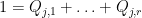 into diagonal projections such that
  lie between and . The eigenvalues of
  are then bounded in magnitude by , and the claim follows by using the partition
 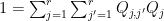 .
.
Finally, we remove the Hermitian condition:
Corollary 27 (Paving conjecture for finite matrices) Let , and let be a matrix with vanishing diagonal, with for some . Then, for any , there exists a partition  of the identity into diagonal projections
  such that
for all  .
.
Proof: By applying the preceding corollary to the Hermitian matrices  and
and  , which both have operator norm at most
  , we may find partitions and
  into diagonal projections such that

and

for all  . In particular,

(note that  commute). The claim then follows from the triangle inequality.
Because the bound here is independent of the dimension , we may use a standard compactness argument to handle infinite matrices:
Corollary 28 (Paving conjecture for infinite matrices) Let  be an infinite matrix with vanishing diagonal, with for some . Then, for any , there exists a partition of the identity into diagonal projections such that
for all .
Proof: For each  , let
, let  be the top minor of , extended by zero to an infinite matrix. This matrix has zeroes on the diagonal and has operator norm at most . Applying Corollary 27 to the
  minor of and then extending, we may find a partition
  into diagonal projections
  such that

for all .
By the Arzela-Ascoli theorem (or the sequential Banach-Alaoglu theorem), we may pass to a subsequence  such that each of the
  converges pointwise to a limit (i.e. each coefficient of the matrix converges as
  to the corresponding coefficient of . As the are diagonal projections, the are as well; since
  , we see on taking pointwise limits that
  .
.
Now let  be unit vectors in
  with finite support. Then
  for sufficiently large
  , and similarly
  . As
. As  and
and  have finite support, we also have
  on the support of for sufficiently large , and hence

for sufficiently large . By (15) and the Cauchy-Schwarz inequality, we conclude that

taking suprema over all unit vectors  we obtain
for all  as required.
— 5. The Kadison-Singer problem —
To turn to the original formulation of the Kadison-Singer problem, we need some terminology from  -algebras. We will work with two specific algebras: the space
  of bounded linear operators on (or equivalently, infinite matrices with bounded operator norm); and the subspace
  of diagonal matrices in
  . These are both examples of -algebras, but we will not need the specific definition of a -algebra in what follows.
A state  on is a bounded linear functional on with
  , such that
  for all positive semi-definite
  . A state is pure if it cannot be represented as a convex combination of two other states. Define a state
  (and a pure state ) similarly.
The Kadison-Singer problem, now solved in the affirmative by Marcus, Spielman, and Srivastava, states the following:
Theorem 29 (Kadison-Singer problem) Let be a pure state. Then there is a unique state  that extends
  . (In particular, this state is automatically pure).
Existence of  is easy: set
  , where
  is the matrix
  with all off-diagonal entries set to zero. The hard part is uniqueness. To solve this problem, let us first understand the structure of pure states on .
Let , and let  be a diagonal projection matrix. Since and
  are both positive semi-definite, we have
  , and hence
  . We in fact claim that either
  or
or  . Indeed, suppose that
  for some
  . Then we can write
  , where
  and
and  . It is easy to see that
  are both states on , contradicting the hypothesis that is pure.
Remark 30 With only a little more effort, this argument shows that the pure states of are in one-to-one correspondence with the ultrafilters of  , but we will not need to use the finer properties of ultrafilters here.
Now we show uniqueness. Let be a state extending . Let ; our task is to show that  . By subtracting off , we may assume that has zero diagonal. Our task is now to show that
  .
.
Let  . By Corollary 28 (with sufficiently large), we may find a partition
  into diagonal projections
  such that

for all  .
.
Recall that  is either or ; since
  , we have
  for exactly one , say
  , and
, and  for all other .
Suppose that  is such that
  . Since
  is a Hermitian semi-definite inner product on , we have the Cauchy-Schwarz inequality

since  , we conclude that
  for all and
  ; similarly
  . We conclude that
  , and hence by (16) we have

where  is the operator norm of . Since may be arbitrarily small, we conclude that as required.


41 comments
Comments feed for this article
4 November, 2013 at 6:43 pm
Anonymous
Your first few references to the authors misspell Nikhil Srivastava’s last name as Srinivasta.
[Corrected, thanks. -T.]
4 November, 2013 at 8:05 pm
DP
In Theorems 6 and 7 the expected value is missing for the trace, and in Theorem 7, the last statement does not agree with the one in Theorem 6. Also, above Theorem 7, the reference is to Proposition 2.
[Corrected, thanks – T.]
5 November, 2013 at 12:11 pm
CO
A few small corrections: Parentheses before 1-\lambda are missing on lines 4, 7 and 8 in the proof of Lemma 14. In Corollary 15, matrices are independent and the inequalities are not strict. In the proof of Corollary 15 – iterating Lemma 14. In the proof of Lemma 17 (first line), the claim follows from Lemma 16.
[Corrected, thanks – T.]
6 November, 2013 at 10:28 pm
Orr Shalit
Thanks for the beautiful post.
A pure state is one that cannot be written as a *convex* combination of other states; one may write some pure states as linear combinations of other states (second paragraph of last section).
[Corrected, thanks – T.]
7 November, 2013 at 12:25 pm
Felix V.
Dear Prof. Tao,
thanks for the beautiful post.
I have a question regarding Lemma 12: It seems to me that real stable polynomials are NOT invariant under restriction. Consider the polynomial p(z_1, z_2) = z_2^2. According to the definition, p is real stable (for every zero, we have z_2 = 0, i.e. (z_1, z_2) is no member of the “upper half plane”).
But if we substitute z_2 = t := 0, then we get p(z_1, t) = 0, which is NOT real stable.
(The application of Rouches Theorem in the proof fails if the polynomial p(z_1, \dots, z_{m-2}, z, t) vanishes identical as a function of z.)
I am sorry if I am making some silly mistake.
Best regards,
Felix V.
[Clarified that the restriction property only holds when the restricted polynomial is not identically zero. (In the applications, all the polynomials are monic in at least one of the variables and so are not identically zero.) -T.]
8 November, 2013 at 6:02 am
DP
z_2^2 is not real stable, for example, it has a root (i, 0).
8 November, 2013 at 10:42 am
DP
Dear Terry,
I think your clarification is a bit confusing and unnecessary. The polynomial can not become identically zero, because the same argument by Rouche’s theorem would imply that the original polynomial was not stable, wouldn’t it?
8 November, 2013 at 11:10 am
DP
Sorry, you are right, I was confused.
14 November, 2013 at 6:44 am
Felix V.
Thank you very much for the clarification.
So an alternative argument (avoiding Rouches’ theorem) would be that p(\cdot, …, \cdot, t + i/n) converges locally uniformly to p(\cdot, …, \cdot, t) and has no zeros on the upper half plane, so that (a multidimensional form of) Hurwitz’ theorem (http://en.wikipedia.org/wiki/Hurwitz%27s_theorem_%28complex_analysis%29#Applications ) implies that p(\cdot, …, \cdot, t) vanishes identically or has no zeros on the upper half plane.
I have another question regarding the proof of lemma 17. You state that by excluding finitely many points, the zeros can be smoothly parameterized. Can you give me a hint on where to look that up or how to show it?
It is clear that the claim follows by the implicit function theorem as long as \frac{\partial}{\partial z_1} p(z_1, z_2) \neq 0 for all zeros z_2 of p(z_1, \cdot), but I don’t see why this should be true for all but finitely many points.
Am I missing something?
Best regards,
Felix V.
14 November, 2013 at 1:37 pm
Felix V.
In my last comment I meant \frac{\partial}{\partial x_2} instead of x_1. This is then of course the same as to say that all zeros have multiplicity one.
As you explicitly state that you do NOT exclude this case (after all, this could happen for ALL x1), I am even more at a loss.
Any help would be appreciated.
Best regards,
Felix V.
14 November, 2013 at 2:22 pm
Terence Tao
Here I am using the fact that an irreducible algebraic curve is smooth at all but finitely many points. (Indeed, if the curve is given by for some irreducible P, then the partial derivatives of P are coprime to P, so by Bezout’s theorem there are only finitely many points where P and
  both vanish.) For similar reasons, there are only finitely many points where the gradient is horizontal, unless the curve is a vertical line (which can be excluded here).
In this setting, P need not be irreducible, but it can be broken up into irreducible components, which again by Bezout only meet each other in finitely many places. (It is possible for components to appear with multiplicity, but then one can just take a single instance of each component, which will still be smooth away from finitely many points.)
p.s. one can certainly use Hurwitz’s theorem here in place of Rouche’s theorem, but the former theorem is often presented as a corollary of the latter, so the arguments are not terribly different from each other.
17 November, 2013 at 2:17 am
Felix V.
Thank you very much. That helped a lot.
2 December, 2013 at 10:55 am
Felix V.
Dear Prof. Tao,
here are a few minor (supposed) mistakes that I found:
In Lemma 12 “the same sign as t” should be “the opposite sign of t”.
In Corollary 15 in the expression “we see that X must lie in the convex hull of the Y” (for appropiate values of X,Y) X and Y should have been interchanged.
In Lemma 16 you mean k! instead of (k-1)! and (x-y_i)^(k+1) instead of (x – y_i)^k.
In Lemma 20 the “convexity estimate” is incorrect. On the right hand side you have to write \partial_j \Phi_q^i (x + \delta e_j) instead of \partial_j Phi_q^i (x). (This replacement has also to be made in the next formula).
In the proof of Theorem 22, the very beginning of the last formula (\Vert) can be removed. In the line before that: “j=1, \dots, r” instead of “j=1,2”.
In the statement of corollary 23: “0s and 1s on the identity” should have been “0s and 1s on the diagonal”.
Minor improvement: In the statement of Corollary 27 it should be possible to replace both 4s by 2s, as you are using the triangle inequality on P = (P + P*)/2 + (P – P*)/2. This can consequently also be done in Corollary 28.
Thanks again for the nice post.
Best regards,
Felix V.
[Corrected, thanks – T.]
8 November, 2013 at 12:29 pm
The Kadison-Singer Conjecture has beed Proved by Adam Marcus, Dan Spielman, and Nikhil Srivastava | Combinatorics and more
[…] Updates: A very nice post on the relation of the Kadison-Singer Conjecture to foundation of quantum mechanics is in this post in Bryan Roberts‘ blog Soul Physics. Here is a very nice post on the mathematics of the conjecture with ten interesting comments on the proof by Orr Shalit, and another nice post on Yemon Choi’s blog. Nov 4, 2013: A new post appeared on Terry tao’s blog, Real stable polynomials and the Kadison Singer Problem. […]
8 November, 2013 at 5:48 pm
Mustafa
There is a typo in Corollary 26: you repeat the “then for r \geq 1.”
[Corrected, thanks – T.]
13 November, 2013 at 2:39 am
TRINH Tuan Phong
Dear Prof. Tao,
May I have a question? I wonder whether “x=(x_1,…,x_m) lies above a root z=(z_1,…,z_m) of the polynomial p” in your note means x_j\geq z_j for some j?
Best regards,
TRINH Tuan Phong
[For all j, not some j; see text before Lemma 17, and also the proof of Lemma 19. -T.]
14 November, 2013 at 4:15 am
TRINH Tuan Phong
Thank you so much for your answer.
Best regards,
T.T.Phong
13 November, 2013 at 5:29 pm
Peter Tobler
Hi – hope you don’t mind me raising this minor point – the guy’s name is Srivastava
[Corrected, thanks – T.]
17 November, 2013 at 9:42 am
Pete Casazza
There is a trivial way to see that paving is equivalent to paving projections with small diagonal. As Teri noted, we may assume T is self-adjoint. Also, we clearly may assume \|T\| \le 1. Now form the square matrix
Since R^2=I, P= 1/2(I+R) is a projection with diagonal 1/2 and we can pave
T if and only if we can pave P. Iterating this, we can reduce to diagonal to
1/2^n with the same conclusion.
18 November, 2013 at 3:38 pm
omar aboura
In theorem 7: $ maxroot E p $ should be $ maxroot (E p) $.
In “…are all geerically non-increasing”, geerically should be generically.
At the end of the proof of Corollary 27, “…commute” should be “…commute)”.
In Corollary 27 and Corollary 28, “for any $r\geq 1$, for any $r\geq 1$” should be “for any $r\geq 1$”.
[Corrected, thanks – T.]
17 April, 2014 at 10:14 pm
Anonymous
http://www.siam.org/prizes/sponsored/polya.php
17 May, 2014 at 10:05 am
Daniel Spielman talks at HUJI – thoughts | Noncommutative Analysis
[…] KS2 conjecture, which implies a positive solution to Kadison-Singer (the full story been worked out to expository perfection on Tao’s […]
19 September, 2014 at 5:39 am
Fall 2014: Roots of polynomials and probabilistic applications | Stochastic Analysis Seminar
[…] Notes by T. Tao […]
13 October, 2014 at 11:10 am
André Schemaitat
In Corollary 28 it is stated that P Q_j u = P^{(m_l)} Q_j u for large l since Q_j u has finite support. Why should this be true ? I.e. if P has many non-zero elements in its rows than P Q_j u won’t even be a vector of finite support.
[Oops, this equality should be restricted to the support of . I’ve updated the text accordingly. -T.]
3 November, 2014 at 8:37 pm
Lecture 5. Proof of Kadison-Singer (3) | Stochastic Analysis Seminar
[…] of the proof of the Kadison-Singer theorem has largely followed the approach from the blog post by T. Tao, which simplifies some of the arguments in the original paper by A. W. Marcus, D. A. Spielman, and […]
6 January, 2015 at 5:45 am
Another one bites the dust (actually many of them) | Noncommutative Analysis
[…] there is Terry Tao’s post on this subject that I read and […]
8 April, 2015 at 10:25 am
jacobcarruth
Reblogged this on jacobcarruth.
16 November, 2016 at 3:53 pm
Anonymous
In the proof of the second part of Lemma 12, why is it sufficient to freeze all but one variable?
16 November, 2016 at 9:23 pm
Terence Tao
A polynomial is stable iff, whenever
  have positive imaginary part, the one-variable polynomial
  is stable.
17 November, 2016 at 3:07 pm
Anonymous (Sheepish)
Oh duh. I think I was confusing “stable” and “real stable.” Anyways thanks, and I think it’s really cool that you replied :)
17 November, 2016 at 8:31 am
bsquare
Hi M.Tao,
TO fix Riemann Zeta function, could we use neural networks to predict
that all solutions are included on a vertical straight line, with good accuracy indeed?
20 November, 2016 at 4:53 am
nassoro mtandani
Hi prof. Tao am so interested in mathematics,please help me where do i start and what should i do?
27 January, 2017 at 10:56 pm
Aleman, Hartz, McCarthy and Richter characterize interpolating sequences in complete Pick spaces | Noncommutative Analysis
[…] A reader familiar with Hilbert function spaces, who takes the paving theorem on faith, can understand the proof immediately after reading Chapter 9 in Agler and McCarthy’s monograph. For a very readable exposition of Kadison-Singer including a proof of the paving theorem (following the work of Marcus-Spielman-Srivastava) see Terry Tao’s blog. […]
24 March, 2019 at 7:52 am
Un lemme de Tao concernant la stabilité réelle | Random Mathematics
[…] This Lemma 14 in Tao’s post here. […]
24 March, 2019 at 5:10 pm
From MSS to Paving | Random Mathematics
[…] From Tao’s post. […]
25 June, 2020 at 8:55 am
tmukblog
Just wondering how does one prove that the expression ${\hbox{det}( z + \sum_{i=1}^m z_i A_i )}$ is a polynomial combination of the ${z_i A_i}$?
25 June, 2020 at 9:38 am
Terence Tao
The determinant function is a polynomial, thus is a polynomial in the (coefficients of the)
  .
.
25 June, 2020 at 11:00 am
Anonymous
Thank you!
12 July, 2020 at 10:36 am
Anonymous
Hello Professor Tao, I actually don’t think I follow Corollary 4 of Proposition 3. In Proposition 3, you show that=p_{A}(z)](https://s0.wp.com/latex.php?latex=%5Cmu%5BA_%7B1%7D%2C+%5Cldots%2C+A_%7Bm%7D%5D%28z%29%3Dp_%7BA%7D%28z%29&bg=ffffff&fg=545454&s=0&c=20201002) and in corollary 4, you consider the case where the
and in corollary 4, you consider the case where the  are random rank one matrices and then assert that
 ![\mu[E[A_{1}, \ldots, E[A_{m}]]=E[p_{A}]](https://s0.wp.com/latex.php?latex=%5Cmu%5BE%5BA_%7B1%7D%2C+%5Cldots%2C+E%5BA_%7Bm%7D%5D%5D%3DE%5Bp_%7BA%7D%5D&bg=ffffff&fg=545454&s=0&c=20201002) . I’m trying to follow the case where
. I’m trying to follow the case where  , in which case we get that
 ![\mu[E[A]](z) = p_{E[A]}(z)](https://s0.wp.com/latex.php?latex=%5Cmu%5BE%5BA%5D%5D%28z%29+%3D+p_%7BE%5BA%5D%7D%28z%29&bg=ffffff&fg=545454&s=0&c=20201002) (from Proposition 3) but
(from Proposition 3) but ![p_{E[A]}(z)](https://s0.wp.com/latex.php?latex=p_%7BE%5BA%5D%7D%28z%29&bg=ffffff&fg=545454&s=0&c=20201002) doesn’t equal
doesn’t equal ![E[p_{A}(z)]](https://s0.wp.com/latex.php?latex=E%5Bp_%7BA%7D%28z%29%5D&bg=ffffff&fg=545454&s=0&c=20201002) ? I thought about the case where
? I thought about the case where  is random with probability 1/2 of being either the projection
 ![[[1,0];[0,0]]](https://s0.wp.com/latex.php?latex=%5B%5B1%2C0%5D%3B%5B0%2C0%5D%5D&bg=ffffff&fg=545454&s=0&c=20201002) to the basis vector
to the basis vector  in the plane or the projection
 ![[[0,0];[0,1]]](https://s0.wp.com/latex.php?latex=%5B%5B0%2C0%5D%3B%5B0%2C1%5D%5D&bg=ffffff&fg=545454&s=0&c=20201002) to the basis vector
to the basis vector  in the plane, in this silly example
 ![E[A]](https://s0.wp.com/latex.php?latex=E%5BA%5D&bg=ffffff&fg=545454&s=0&c=20201002) is the diagonal matrix with
is the diagonal matrix with  on the diagonal entries whose char. polynomial is
  while
while ![E[p_{A}]=z(z-1)](https://s0.wp.com/latex.php?latex=E%5Bp_%7BA%7D%5D%3Dz%28z-1%29&bg=ffffff&fg=545454&s=0&c=20201002) . So I must of misunderstood an assumption. As far as the proof given, I think I don’t quite see what happens after you take expectation on both sides. Sorry for the long post and for the latex errors (maybe I should have asked this on MO)
. So I must of misunderstood an assumption. As far as the proof given, I think I don’t quite see what happens after you take expectation on both sides. Sorry for the long post and for the latex errors (maybe I should have asked this on MO)
17 July, 2020 at 5:41 pm
Terence Tao
In your example you will not in fact have![\mu[E[A]](z)](https://s0.wp.com/latex.php?latex=%5Cmu%5BE%5BA%5D%5D%28z%29&bg=ffffff&fg=545454&s=0&c=20201002) equal to
equal to ![p_{E[A]}(z)](https://s0.wp.com/latex.php?latex=p_%7BE%5BA%5D%7D%28z%29&bg=ffffff&fg=545454&s=0&c=20201002) because
because ![E[A]](https://s0.wp.com/latex.php?latex=E%5BA%5D&bg=ffffff&fg=545454&s=0&c=20201002) is not a rank 1 matrix. Instead,
is not a rank 1 matrix. Instead, ![\mu[E[A]](z)](https://s0.wp.com/latex.php?latex=%5Cmu%5BE%5BA%5D%5D%28z%29&bg=ffffff&fg=545454&s=0&c=20201002) is equal by definition to
is equal by definition to
as claimed.
18 July, 2020 at 9:18 am
Anonymous
Oh I see. We need rank one to apply Proposition 3. Thank you for clarifying. I think I understand the proof a little better now.