
You are currently browsing the tag archive for the ‘random matrices’ tag.
This is another sequel to a recent post in which I showed the Riemann zeta function 
![{t \in [T,2T]}](https://s0.wp.com/latex.php?latex=%7Bt+%5Cin+%5BT%2C2T%5D%7D&bg=ffffff&fg=000000&s=0&c=20201002)

where 


In this post I would like to record this analogue precisely. We will need a finite field 


We will primarily think of ![{{\mathbb F}[X]}](https://s0.wp.com/latex.php?latex=%7B%7B%5Cmathbb+F%7D%5BX%5D%7D&bg=ffffff&fg=000000&s=0&c=20201002)

![{{\mathbb F}[X]'}](https://s0.wp.com/latex.php?latex=%7B%7B%5Cmathbb+F%7D%5BX%5D%27%7D&bg=ffffff&fg=000000&s=0&c=20201002)

![{n \in {\mathbb F}[X]}](https://s0.wp.com/latex.php?latex=%7Bn+%5Cin+%7B%5Cmathbb+F%7D%5BX%5D%7D&bg=ffffff&fg=000000&s=0&c=20201002)

![{Q \in {\mathbb F}[X]}](https://s0.wp.com/latex.php?latex=%7BQ+%5Cin+%7B%5Cmathbb+F%7D%5BX%5D%7D&bg=ffffff&fg=000000&s=0&c=20201002)


![{({\mathbb F}[X]/Q{\mathbb F}[X])^\times}](https://s0.wp.com/latex.php?latex=%7B%28%7B%5Cmathbb+F%7D%5BX%5D%2FQ%7B%5Cmathbb+F%7D%5BX%5D%29%5E%5Ctimes%7D&bg=ffffff&fg=000000&s=0&c=20201002)

![{\chi: {\mathbb F}[X] \rightarrow {\bf C}}](https://s0.wp.com/latex.php?latex=%7B%5Cchi%3A+%7B%5Cmathbb+F%7D%5BX%5D+%5Crightarrow+%7B%5Cbf+C%7D%7D&bg=ffffff&fg=000000&s=0&c=20201002)


Let 


![\displaystyle L(s,\chi) := \sum_{n \in {\mathbb F}[X]'} \frac{\chi(n)}{|n|^s}](https://s0.wp.com/latex.php?latex=%5Cdisplaystyle++L%28s%2C%5Cchi%29+%3A%3D+%5Csum_%7Bn+%5Cin+%7B%5Cmathbb+F%7D%5BX%5D%27%7D+%5Cfrac%7B%5Cchi%28n%29%7D%7B%7Cn%7C%5Es%7D&bg=ffffff&fg=000000&s=0&c=20201002)
![\displaystyle = \sum_{m=0}^\infty q^{-sm} \sum_{n \in {\mathbb F}[X]': |n| = q^m} \chi(n).](https://s0.wp.com/latex.php?latex=%5Cdisplaystyle++%3D+%5Csum_%7Bm%3D0%7D%5E%5Cinfty+q%5E%7B-sm%7D+%5Csum_%7Bn+%5Cin+%7B%5Cmathbb+F%7D%5BX%5D%27%3A+%7Cn%7C+%3D+q%5Em%7D+%5Cchi%28n%29.&bg=ffffff&fg=000000&s=0&c=20201002)
Note that for 
![{n \in {\mathbb F}[X]': |n| = q^m}](https://s0.wp.com/latex.php?latex=%7Bn+%5Cin+%7B%5Cmathbb+F%7D%5BX%5D%27%3A+%7Cn%7C+%3D+q%5Em%7D&bg=ffffff&fg=000000&s=0&c=20201002)


![{{\mathbb F}[X]/Q{\mathbb F}[X]}](https://s0.wp.com/latex.php?latex=%7B%7B%5Cmathbb+F%7D%5BX%5D%2FQ%7B%5Cmathbb+F%7D%5BX%5D%7D&bg=ffffff&fg=000000&s=0&c=20201002)
![{\sum_{n \in {\mathbb F}[X]': |n| = q^m} \chi(n)}](https://s0.wp.com/latex.php?latex=%7B%5Csum_%7Bn+%5Cin+%7B%5Cmathbb+F%7D%5BX%5D%27%3A+%7Cn%7C+%3D+q%5Em%7D+%5Cchi%28n%29%7D&bg=ffffff&fg=000000&s=0&c=20201002)


where 

![\displaystyle c^1_m(t,\chi) := q^{-m/2-imt} \sum_{n \in {\mathbb F}[X]': |n| = q^m} \chi(n).](https://s0.wp.com/latex.php?latex=%5Cdisplaystyle++c%5E1_m%28t%2C%5Cchi%29+%3A%3D+q%5E%7B-m%2F2-imt%7D+%5Csum_%7Bn+%5Cin+%7B%5Cmathbb+F%7D%5BX%5D%27%3A+%7Cn%7C+%3D+q%5Em%7D+%5Cchi%28n%29.&bg=ffffff&fg=000000&s=0&c=20201002)
Note that

In particular, the dependence on 

Fourier inversion yields a functional equation for the polynomial 
Proposition 1 (Functional equation) Let
. There exists a phase
(depending on
) such that
for all
, or equivalently that
where
.
Proof: We can normalise 

![{{\mathbb F}[X] / Q {\mathbb F}[X]}](https://s0.wp.com/latex.php?latex=%7B%7B%5Cmathbb+F%7D%5BX%5D+%2F+Q+%7B%5Cmathbb+F%7D%5BX%5D%7D&bg=ffffff&fg=000000&s=0&c=20201002)
where 


where
From change of variables we see that 

for some phase 

The inner sum 


For 


By the multiplicativity of

From the one-dimensional version of (3) (and the fact that

for some phase 

As one corollary of the functional equation, 

Theorem 2 (Riemann hypothesis for Dirichlet
We derive this result from the Riemann hypothesis for curves over function fields below the fold.
In view of this theorem (and the fact that 

for some unitary 


We now let 

If one lets 

and hence the 

One can take log derivatives to conclude
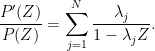
On the other hand, as in the number field case one has the Dirichlet series expansion
![\displaystyle Z \frac{P'(Z)}{P(Z)} = \sum_{n \in {\mathbb F}[X]'} \frac{\Lambda_q(n) \chi(n)}{|n|^s}](https://s0.wp.com/latex.php?latex=%5Cdisplaystyle++Z+%5Cfrac%7BP%27%28Z%29%7D%7BP%28Z%29%7D+%3D+%5Csum_%7Bn+%5Cin+%7B%5Cmathbb+F%7D%5BX%5D%27%7D+%5Cfrac%7B%5CLambda_q%28n%29+%5Cchi%28n%29%7D%7B%7Cn%7C%5Es%7D&bg=ffffff&fg=000000&s=0&c=20201002)
where 


for 
![\displaystyle c^{\Lambda_q}_m := q^{-m/2-imt} \sum_{n \in {\mathbb F}[X]': |n| = q^m} \Lambda_q(n) \chi(n).](https://s0.wp.com/latex.php?latex=%5Cdisplaystyle++c%5E%7B%5CLambda_q%7D_m+%3A%3D+q%5E%7B-m%2F2-imt%7D+%5Csum_%7Bn+%5Cin+%7B%5Cmathbb+F%7D%5BX%5D%27%3A+%7Cn%7C+%3D+q%5Em%7D+%5CLambda_q%28n%29+%5Cchi%28n%29.&bg=ffffff&fg=000000&s=0&c=20201002)
Similarly on inverting 

Since we also have
![\displaystyle P(Z)^{-1} = \sum_{n \in {\mathbb F}[X]'} \frac{\mu(n) \chi(n)}{|n|^s}](https://s0.wp.com/latex.php?latex=%5Cdisplaystyle++P%28Z%29%5E%7B-1%7D+%3D+%5Csum_%7Bn+%5Cin+%7B%5Cmathbb+F%7D%5BX%5D%27%7D+%5Cfrac%7B%5Cmu%28n%29+%5Cchi%28n%29%7D%7B%7Cn%7C%5Es%7D&bg=ffffff&fg=000000&s=0&c=20201002)
for 


![\displaystyle c^\mu_m := q^{-m/2-imt} \sum_{n \in {\mathbb F}[X]': |n| = q^m} \mu(n) \chi(n)](https://s0.wp.com/latex.php?latex=%5Cdisplaystyle++c%5E%5Cmu_m+%3A%3D+q%5E%7B-m%2F2-imt%7D+%5Csum_%7Bn+%5Cin+%7B%5Cmathbb+F%7D%5BX%5D%27%3A+%7Cn%7C+%3D+q%5Em%7D+%5Cmu%28n%29+%5Cchi%28n%29&bg=ffffff&fg=000000&s=0&c=20201002)
are just the complete homogeneous symmetric polynomials of the eigenvalues:

One can then derive various algebraic relationships between the coefficients 
What do we know about the distribution of 

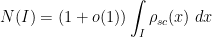
Proposition 3 (Rudnick-Sarnak asymptotics) Let
be nonnegative integers. If
is equal to
in the limit
fixed) unless
for all


Comparing this with Proposition 1 from this previous post, we thus see that all the low moments of 
Proof: We may assume the homogeneity relationship

since otherwise the claim follows from the invariance under phase rotation 
![\displaystyle q^{-D} {\bf E}_Q \sum_{n_1,\dots,n_l,n'_1,\dots,n'_{l'} \in {\mathbb F}[X]': |n_i| = q^{s_i}, |n'_i| = q^{s'_i}} (\prod_{i=1}^l \Lambda_q(n_i) \chi(n_i)) \prod_{i=1}^{l'} \Lambda_q(n'_i) \overline{\chi(n'_i)}](https://s0.wp.com/latex.php?latex=%5Cdisplaystyle++q%5E%7B-D%7D+%7B%5Cbf+E%7D_Q+%5Csum_%7Bn_1%2C%5Cdots%2Cn_l%2Cn%27_1%2C%5Cdots%2Cn%27_%7Bl%27%7D+%5Cin+%7B%5Cmathbb+F%7D%5BX%5D%27%3A+%7Cn_i%7C+%3D+q%5E%7Bs_i%7D%2C+%7Cn%27_i%7C+%3D+q%5E%7Bs%27_i%7D%7D+%28%5Cprod_%7Bi%3D1%7D%5El+%5CLambda_q%28n_i%29+%5Cchi%28n_i%29%29+%5Cprod_%7Bi%3D1%7D%5E%7Bl%27%7D+%5CLambda_q%28n%27_i%29+%5Coverline%7B%5Cchi%28n%27_i%29%7D&bg=ffffff&fg=000000&s=0&c=20201002)
where


and 


The polynomials 


vanishes unless 

There are at most 


![\displaystyle q^{-D} \prod_{j=1}^k j a_j! \sum_{n_1,\dots,n_l,n'_1,\dots,n'_{l'}\in {\mathbb F}[X]': |n_i| = q^{s_i}} \prod_{i=1}^l \Lambda_q(n_i) + o(1).](https://s0.wp.com/latex.php?latex=%5Cdisplaystyle++q%5E%7B-D%7D+%5Cprod_%7Bj%3D1%7D%5Ek+j+a_j%21+%5Csum_%7Bn_1%2C%5Cdots%2Cn_l%2Cn%27_1%2C%5Cdots%2Cn%27_%7Bl%27%7D%5Cin+%7B%5Cmathbb+F%7D%5BX%5D%27%3A+%7Cn_i%7C+%3D+q%5E%7Bs_i%7D%7D+%5Cprod_%7Bi%3D1%7D%5El+%5CLambda_q%28n_i%29+%2B+o%281%29.&bg=ffffff&fg=000000&s=0&c=20201002)
Using the prime number theorem ![{\sum_{n \in {\mathbb F}[X]': |n| = q^s} \Lambda_q(n) = q^s}](https://s0.wp.com/latex.php?latex=%7B%5Csum_%7Bn+%5Cin+%7B%5Cmathbb+F%7D%5BX%5D%27%3A+%7Cn%7C+%3D+q%5Es%7D+%5CLambda_q%28n%29+%3D+q%5Es%7D&bg=ffffff&fg=000000&s=0&c=20201002)
Comparing this with Proposition 1 from this previous post, we thus see that all the low moments of
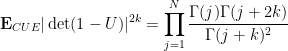
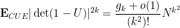
Corollary 4 (CUE statistics at low frequencies) Let
be a linear combination of monomials
where
are integers with either
or
. Then

The analogue of the GUE hypothesis in this setting would be the CUE hypothesis, which asserts that the threshold 

Proof: By permutation symmetry we can take 


Thus, for instance, for 


is equal to

because all the monomials in 

of Baker-Forrester and Keating-Snaith, thus for instance


and more generally
when 


and more generally
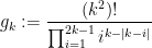
(OEIS A039622). Thus we have

for 
Now we can recover the analogue of Montgomery’s work on the pair correlation conjecture. Consider the statistic
where

is some finite linear combination of monomials 
Assuming the CUE hypothesis, then by Example 3 of the previous post, we would conclude that

This is the analogue of Montgomery’s pair correlation conjecture. Proposition 3 implies that this claim is true whenever 
![{[-N,N]}](https://s0.wp.com/latex.php?latex=%7B%5B-N%2CN%5D%7D&bg=ffffff&fg=000000&s=0&c=20201002)


for arbitrary 

if 

By applying (12) for various choices of test functions

Then (12) applies unconditionally and we conclude that

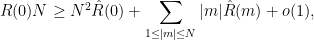
The right-hand side evaluates to 


The sum 


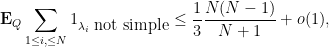
and thus the expected number of simple eigenvalues is at least 

Suppose that the phase gaps in 


![{[-c/N,c/N]}](https://s0.wp.com/latex.php?latex=%7B%5B-c%2FN%2Cc%2FN%5D%7D&bg=ffffff&fg=000000&s=0&c=20201002)
so by taking contrapositives one can force the existence of a gap less than

By a suitable choice of 


In some cases it is possible to go beyond Proposition 3. Consider the mollified moment

where

for some coefficients 
Proposition 5 We have

Proof: From (5) one has

hence

where we suppress the dependence on the eigenvalues 

where 
and we adopt the convention that 


As the Schur polynomials are orthonormal on the unitary group, the claim follows.
The CUE hypothesis would then imply the corresponding mollified moment conjecture

(See this paper of Conrey, and this paper of Radziwill, for some discussion of the analogous conjecture for the zeta function, which is essentially due to Farmer.)
From Proposition 3 one sees that this conjecture holds in the range 


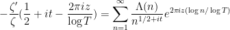
In a recent post I discussed how the Riemann zeta function
where 

Here 

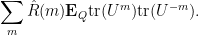
Taking logarithmic derivatives of (2), we have

and hence on taking logarithmic derivatives of (1) in the

Morally speaking, we have
so on comparing coefficients we expect to interpret the moments 
To understand the distribution of

where 


where 

The moment (6) vanishes unless one has the homogeneity condition

This follows from the fact that for any phase 


In the case when the degree 
Proposition 1 (Low moments in CUE model) If
then the moment (6) vanishes unless

Another way of viewing this proposition is that for 
Proof: Let

Our starting point is Schur-Weyl duality. Namely, we consider the 

This space has an action of the product group 


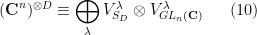
where 

Let 


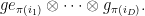
The trace of this action can then be computed as
where 


But we can also compute this trace using the Schur-Weyl decomposition (10), yielding the identity

where 


and similarly

where 


Now recall that 


Example 2 We illustrate the identity (11) when
,
. The Schur polynomials are given as
where
are the (generalised) eigenvalues of
The functions
are orthonormal on
are also, and their
norms are
,
, and
respectively, reflecting the size in
of the centralisers of the permutations
,
, and
respectively. If
terms now disappear (the Young tableau here has too many rows), and the three quantities here now have some non-trivial covariance.


Example 3 Consider the moment
. For
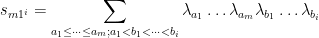
, the above proposition shows us that this moment is equal to
? The formula (12) computes this moment as
where
, and
vanishes unless
of vectors in
whose coordinates sum to zero), in which case it is equal to
(depending on the parity of the number of non-zero rows). As such we see that this moment is equal to


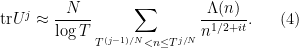
Now we discuss what is known for the analogous moments (5). Here we shall be rather non-rigorous, in particular ignoring an annoying “Archimedean” issue that the product of the ranges 


![{[T,2T]}](https://s0.wp.com/latex.php?latex=%7B%5BT%2C2T%5D%7D&bg=ffffff&fg=000000&s=0&c=20201002)
One can morally expand out (5) using (4) as


where 


for 

for 

in which case the expecation is oscillates with magnitude one. In particular, if (7) fails (with some room to spare) then the moment (5) should be negligible, which is consistent with the analogous behaviour for the moments (6). Now suppose that (8) holds (with some room to spare). Then 


The von Mangoldt factors 


and using Mertens’ theorem this soon simplifies asymptotically to the same quantity in Proposition 1. Thus we see that (morally at least) the moments (5) associated to the zeta function asymptotically match the moments (6) coming from the CUE model in the low degree case (8), thus lending support to the GUE hypothesis. (These observations are basically due to Rudnick and Sarnak, with the degree
With some rare exceptions (such as those estimates coming from “Kloostermania”), the moment estimates of Rudnick and Sarnak basically represent the state of the art for what is known for the moments (5). For instance, Montgomery’s pair correlation conjecture, in our language, is basically the analogue of (13) for 

for all 
These estimates can be used to give some non-trivial information on the largest and smallest spacings between zeroes of the zeta function, which in our notation corresponds to spacing between eigenvalues of 


then the arcs 


for sufficiently small 


It would be of great interest if one could push the upper bound 


Unfortunately, the known methods do not seem to break this barrier without some significant new input; already the original paper of Montgomery and Odlyzko observed this limitation for their particular technique (and in fact fall very slightly short, as observed in unpublished work of Goldston and of Milinovich). In this post I would like to record another way to see this, by providing an “alternative” probability distribution to the CUE distribution (which one might dub the Alternative Circular Unitary Ensemble (ACUE) which is indistinguishable in low moments in the sense that the expectation 
To describe this alternative distribution, let us first recall the Weyl description of the CUE measure on the unitary group 
where

is the Vandermonde determinant; see for instance this previous blog post for the derivation of a very similar formula for the GUE distribution, which can be adapted to CUE without much difficulty. To see that this is a probability measure, first observe the Vandermonde determinant identity

where 


For the alternative distribution, we first draw 


shift by a phase 


From construction it is clear that the matrix

when 


By Fourier decomposition, it then suffices to show that the trigonometric polynomial 


Example 4 If
, then the distribution (21) assigns a probability of
to any pair
that is a permuted rotation of
, and a probability of
to any pair that is a permuted rotation of
. Thus, a matrix
with probability
with probability
A similar computation when
gives
with probability
, to a phase rotation of
or its adjoint with probability of
each, and a phase rotation of
with probability
.
Remark 5 For large
In some cases, even just a tiny improvement in known results would be able to exclude the alternative hypothesis. For instance, if the alternative hypothesis held, then 

which differs from (13) for any 
Remark 6 One can view the CUE as normalised Lebesgue measure on
). One can similarly view ACUE as normalised Lebesgue measure on the (disconnected) smooth submanifold of
(or one can equivalently take
; in a similar spirit, the phases of ACUE eigenvalues, once they are rotated to be
). In particular, the
.
Remark 7 One family of estimates that go beyond the Rudnick-Sarnak family of estimates are twisted moment estimates for the zeta function, such as ones that give asymptotics for
for some small even exponent
(almost always
) and some short Dirichlet polynomial
where
to cancel the corresponding powers of
). Unfortunately such averages generally are unable to distinguish the CUE from the ACUE. For instance, if all the coefficients of
of total order less than
, then in terms of the eigenvalue phases
is a linear combination of plane waves
where the frequencies
is a linear combination of plane waves
is a linear combination of plane waves where the frequencies
by the previous arguments. In other words,


Remark 8 The GUE hypothesis for the zeta function asserts that the average
for any
and any test function
, where
is the Dyson sine kernel and
are the ordinates of zeroes of the zeta function. This corresponds to the CUE distribution for
This is a stronger version of the alternative hypothesis that the spacing between adjacent zeroes is almost always approximately a half-integer multiple of the mean spacing. I do not know of any known moment estimates for Dirichlet series that is able to eliminate this AGUE hypothesis (even assuming GRH). (UPDATE: These facts have also been independently observed in forthcoming work of Lagarias and Rodgers.)


In July I will be spending a week at Park City, being one of the mini-course lecturers in the Graduate Summer School component of the Park City Summer Session on random matrices. I have chosen to give some lectures on least singular values of random matrices, the circular law, and the Lindeberg exchange method in random matrix theory; this is a slightly different set of topics than I had initially advertised (which was instead about the Lindeberg exchange method and the local relaxation flow method), but after consulting with the other mini-course lecturers I felt that this would be a more complementary set of topics. I have uploaded an draft of my lecture notes (some portion of which is derived from my monograph on the subject); as always, comments and corrections are welcome.
[Update, June 23: notes revised and reformatted to PCMI format. -T.]
[Update, Mar 19 2018: further revision. -T.]
Van Vu and I have just uploaded to the arXiv our paper “Random matrices have simple spectrum“. Recall that an 
For discrete random matrix ensembles, though, the above argument breaks down, even though general universality heuristics predict that the statistics of discrete ensembles should behave similarly to those of continuous ensembles. A model case here is the adjacency matrix 

Our argument works for more general Wigner-type matrix ensembles, but for sake of illustration we will stick with the Erdös-Renyi case. Previous work on local universality for such matrix models (e.g. the work of Erdos, Knowles, Yau, and Yin) was able to show that any individual eigenvalue gap 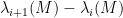


Our argument in fact gives simplicity of the spectrum with probability 

The basic idea of argument can be sketched as follows. Suppose that

for a random 

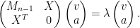
Extracting the top 
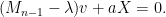
If we let 

we typically expect 

In other words, in order for
[These are notes intended mostly for myself, as these topics are useful in random matrix theory, but may be of interest to some readers also. -T.]
One of the most fundamental partial differential equations in mathematics is the heat equation
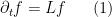
where 

In probability theory, this equation takes on particular significance when 
for all 
where 

A model example of a solution to the heat equation to keep in mind is that of the fundamental solution

defined for any 


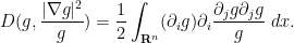
The heat equation can also be viewed as the gradient flow for the Dirichlet form
since one has the integration by parts identity

for all smooth, rapidly decreasing 


For instance, for the fundamental solution (3), one can verify for any time
(assuming I have not made a mistake in the calculation). In a similar spirit we have
Since 


Since 

for any function
There are other quantities relating to
Thus, for instance, if 


A short formal computation shows (if one assumes for simplicity that
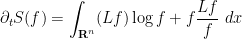


where 

In particular, the entropy is decreasing, which corresponds well to one’s intuition that the heat equation (or Brownian motion) should serve to spread out a probability distribution over time.
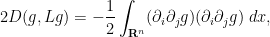
Actually, one can say more: the rate of decrease 

valid for for any smooth function 
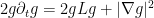
and thus (again assuming that

We thus have
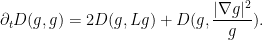
It is now convenient to compute using the Einstein summation convention to hide the summation over indices 
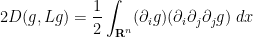
and
By integration by parts and interchanging partial derivatives, we may write the first integral as
and from the quotient and product rules, we may write the second integral as

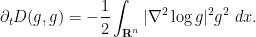
Gathering terms, completing the square, and making the summations explicit again, we see that

and so in particular 
The above identity can also be written as
Exercise 1 Give an alternate proof of the above identity by writing
,
and deriving the equation
for
.
It was observed in a well known paper of Bakry and Emery that the above monotonicity properties hold for a much larger class of heat flow-type equations, and lead to a number of important relations between energy and entropy, such as the log-Sobolev inequality of Gross and of Federbush, and the hypercontractivity inequality of Nelson; we will discuss one such family of generalisations (or more precisely, variants) below the fold.
Van Vu and I have just uploaded to the arXiv our paper “Random matrices: Universality of local spectral statistics of non-Hermitian matrices“. The main result of this paper is a “Four Moment Theorem” that establishes universality for local spectral statistics of non-Hermitian matrices with independent entries, under the additional hypotheses that the entries of the matrix decay exponentially, and match moments with either the real or complex gaussian ensemble to fourth order. This is the non-Hermitian analogue of a long string of recent results establishing universality of local statistics in the Hermitian case (as discussed for instance in this recent survey of Van and myself, and also in several other places).
The complex case is somewhat easier to describe. Given a (non-Hermitian) random matrix ensemble 


In the case when 


for 

for 


(There is also an asymptotic for the boundary case 

Our first main result is that the asymptotic (1) for 

There are several steps involved in the proof. The first step is to apply the Girko Hermitisation trick to replace the problem of understanding the spectrum of a non-Hermitian matrix, with that of understanding the spectrum of various Hermitian matrices. The two identities that realise this trick are, firstly, Jensen’s formula

that relates the local distribution of eigenvalues to the log-determinants 

that relates the log-determinants of 

The main difficulty is then to obtain concentration and universality results for the Hermitian log-determinants 
The matrices 
While this result is the first local universality result in the category of random matrices with independent entries, there are still two limitations to the result which one would like to remove. The first is the moment matching hypotheses on the matrix. Very recently, one of the ingredients of our paper, namely the local circular law, was proved without moment matching hypotheses by Bourgade, Yau, and Yin (provided one stays away from the edge of the spectrum); however, as of this time of writing the other main ingredient – the universality of the log-determinant – still requires moment matching. (The standard tool for obtaining universality without moment matching hypotheses is the heat flow method (and more specifically, the local relaxation flow method), but the analogue of Dyson Brownian motion in the non-Hermitian setting appears to be somewhat intractible, being a coupled flow on both the eigenvalues and eigenvectors rather than just on the eigenvalues alone.)
Van Vu and I have just uploaded to the arXiv our paper Random matrices: Sharp concentration of eigenvalues, submitted to the Electronic Journal of Probability. As with many of our previous papers, this paper is concerned with the distribution of the eigenvalues 


If we normalise the entries of the matrix 

An essentially equivalent way of saying this is that for large 
![{\gamma_i \in [-2,2]}](https://s0.wp.com/latex.php?latex=%7B%5Cgamma_i+%5Cin+%5B-2%2C2%5D%7D&bg=ffffff&fg=000000&s=0&c=20201002)

In particular, from the Wigner semicircle law it can be shown that asymptotically almost surely, one has

for all 
In the modern study of the spectrum of Wigner matrices (and in particular as a key tool in establishing universality results), it has become of interest to improve the error term in (1) as much as possible. A typical early result in this direction was by Bai, who used the Stieltjes transform method to obtain polynomial convergence rates of the shape 


A significant advance in this direction was achieved by Erdos, Schlein, and Yau in a series of papers where they used a combination of Stieltjes transform and concentration of measure methods to obtain local semicircle laws which showed, among other things, that one had asymptotics of the form
with exponentially high probability for intervals 


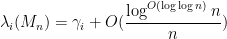
in the bulk with exponentially high probability, for Wigner matrices obeying some exponential decay conditions on the entries. This was achieved by a rather delicate high moment calculation, in which the contribution of the diagonal entries of the resolvent (whose average forms the Stieltjes transform) was shown to mostly cancel each other out.
As the GUE computations show, this concentration result is sharp up to the quasilogarithmic factor 
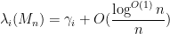
with exponentially high probability (see the paper for a more precise statement of results). The one catch is that an additional hypothesis is required, namely that the entries of the Wigner matrix have vanishing third moment. We also obtain similar results for the edge of the spectrum (but with a different scaling).
Our arguments are rather different from those of Erdos, Yau, and Yin, and thus provide an alternate approach to establishing eigenvalue concentration. The main tool is the Lindeberg exchange strategy, which is also used to prove the Four Moment Theorem (although we do not directly invoke the Four Moment Theorem in our analysis). The main novelty is that this exchange strategy is now used to establish large deviation estimates (i.e. exponentially small tail probabilities) rather than universality of the limiting distribution. Roughly speaking, the basic point is as follows. The Lindeberg exchange strategy seeks to compare a function 


for various smooth test functions 

for various thresholds 
for various moderately large 

after performing all the relevant exchanges. As such, one can then use large deviation estimates on
In this paper we also take advantage of a simplification, first noted by Erdos, Yau, and Yin, that Four Moment Theorems become somewhat easier to prove if one works with resolvents 

for any energy level 


Van Vu and I have just uploaded to the arXiv our short survey article, “Random matrices: The Four Moment Theorem for Wigner ensembles“, submitted to the MSRI book series, as part of the proceedings on the MSRI semester program on random matrix theory from last year. This is a highly condensed version (at 17 pages) of a much longer survey (currently at about 48 pages, though not completely finished) that we are currently working on, devoted to the recent advances in understanding the universality phenomenon for spectral statistics of Wigner matrices. In this abridged version of the survey, we focus on a key tool in the subject, namely the Four Moment Theorem which roughly speaking asserts that the statistics of a Wigner matrix depend only on the first four moments of the entries. We give a sketch of proof of this theorem, and two sample applications: a central limit theorem for individual eigenvalues of a Wigner matrix (extending a result of Gustavsson in the case of GUE), and the verification of a conjecture of Wigner, Dyson, and Mehta on the universality of the asymptotic k-point correlation functions even for discrete ensembles (provided that we interpret convergence in the vague topology sense).
For reasons of space, this paper is very far from an exhaustive survey even of the narrow topic of universality for Wigner matrices, but should hopefully be an accessible entry point into the subject nevertheless.
Van Vu and I have just uploaded to the arXiv our paper “The Wigner-Dyson-Mehta bulk universality conjecture for Wigner matrices“, submitted to the Proceedings of the National Academy of Sciences. This short note concerns the convergence of the 
More precisely, let 


In particular, this suggests that at any energy level 

for any distinct reals 

![{[u + \frac{t_i}{n \rho_{sc}(u)}, u + \frac{t_i+\epsilon}{n \rho_{sc}(u)}]}](https://s0.wp.com/latex.php?latex=%7B%5Bu+%2B+%5Cfrac%7Bt_i%7D%7Bn+%5Crho_%7Bsc%7D%28u%29%7D%2C+u+%2B+%5Cfrac%7Bt_i%2B%5Cepsilon%7D%7Bn+%5Crho_%7Bsc%7D%28u%29%7D%5D%7D&bg=ffffff&fg=000000&s=0&c=20201002)


The Wigner-Dyson-Mehta conjecture asserts that

where 

for any 
In a joint paper of Erdos, Ramirez, Schlein, Vu, Yau, and myself, we established the Wigner-Dyson-Mehta conjecture for all Wigner matrices (assuming only an exponential decay condition on the entries), but using a quite weak notion of convergence, namely averaged vague convergence, which allows for averaging in the energy parameter. Specifically, we showed that

Subsequently, Erdos, Schlein, and Yau introduced the powerful local relaxation flow method, which achieved a simpler proof of the same result which also generalised to other ensembles beyond the Wigner case. However, for technical reasons, this method was restricted to establishing averaged vague convergence only.
In the current paper, we show that by combining the argument of Erdos, Ramirez, Schlein, Vu, Yau, and myself with some more recent technical results, namely the relaxation of the exponential decay condition in the four moment theorem to a finite moment condition (established by Vu and myself) and a strong eigenvalue localisation bound of Erdos, Yau, and Yin, one can upgrade the averaged vague convergence to vague convergence, and handle all Wigner matrices that assume a finite moment condition. Vague convergence is the most natural notion of convergence for discrete random matrix ensembles; for such ensembles, the correlation function is a discrete measure, and so one does not expect convergence to a continuous limit in any stronger sense than the vague sense. Also, by carefully inspecting the earlier argument of Erdos, Peche, Ramirez, Schlein, and Yau, we were able to establish convergence in the stronger local
It may well be possible to go beyond local 
I’ve just uploaded to the arXiv my paper “Outliers in the spectrum of iid matrices with bounded rank perturbations“, submitted to Probability Theory and Related Fields. This paper is concerned with outliers to the circular law for iid random matrices. Recall that if 


The circular law is also stable under bounded rank perturbations: if 


However, this leaves open the possibility for one or more outlier eigenvalues that lie significantly outside the unit disk; the arguments in the paper cited above give some upper bound on the number of such eigenvalues (of the form 
In this paper, some results are given as to when outliers exist, and how they are distributed. The easiest case is of course when there is no bounded rank perturbation: 

Now we consider a bounded rank perturbation 


Thus, for instance, adding a bounded nilpotent low rank matrix to
When I first thought about this problem (which was communicated to me by Larry Abbott), I believed that it was quite difficult, because I knew that the eigenvalues of non-Hermitian matrices were quite unstable with respect to general perturbations (as discussed in this previous blog post), and that there were no interlacing inequalities in this case to control bounded rank perturbations (as discussed in this post). However, as it turns out I had arrived at the wrong conclusion, especially in the exterior of the unit disk in which the resolvent is actually well controlled and so there is no pseudospectrum present to cause instability. This was pointed out to me by Alice Guionnet at an AIM workshop last week, after I had posed the above question during an open problems session. Furthermore, at the same workshop, Percy Deift emphasised the point that the basic determinantal identity

for 


From this, it turned out to be a relatively simple manner to transform what appeared to be an intractable 


This is an 

Now we apply the crucial identity (1) to rearrange this as

The crucial point is that this is now an equation involving only a

in which case the eigenvalue equation is now just a scalar equation

that involves what is basically a single coefficient of the resolvent 
The same method can handle some other bounded rank perturbations. One basic example comes from looking at iid matrices with a non-zero mean 


If one moves away from the case of self-adjoint perturbations, though, the situation changes. Let us now consider a matrix of the form 


where 

On the other hand, as already observed numerically (and rigorously, in the gaussian case) by Rajan and Abbott, if one projects such matrices to have row sum zero, then the outliers all disappear. This can be explained by another appeal to (1); this projection amounts to right-multiplying 


Recent Comments