246B, Notes 3: Elliptic functions and modular forms

2 February, 2021 in 246B - complex analysis, math.CV, math.NT | Tags: complex tori, elliptic curves, j-invariant, modular discriminant, modular forms, modular functions, Weierstrass elliptic function | by Terence Tao

Previous set of notes: Notes 2. Next set of notes: Notes 4.

On the real line, the quintessential examples of a periodic function are the (normalised) sine and cosine functions ${\sin(2\pi x)}$ , ${\cos(2\pi x)}$ , which are ${1}$ -periodic in the sense that

$\displaystyle \sin(2\pi(x+1)) = \sin(2\pi x); \quad \cos(2\pi (x+1)) = \cos(2\pi x).$

By taking various polynomial combinations of ${\sin(2\pi x)}$ and ${\cos(2\pi x)}$ we obtain more general trigonometric polynomials that are ${1}$ -periodic; and the theory of Fourier series tells us that all other ${1}$ -periodic functions (with reasonable integrability conditions) can be approximated in various senses by such polynomial combinations. Using Euler’s identity, one can use ${e^{2\pi ix}}$ and ${e^{-2\pi ix}}$ in place of ${\sin(2\pi x)}$ and ${\cos(2\pi x)}$ as the basic generating functions here, provided of course one is willing to use complex coefficients instead of real ones. Of course, by rescaling one can also make similar statements for other periods than ${1}$ . ${1}$ -periodic functions ${f: {\bf R} \rightarrow {\bf C}}$ can also be identified (by abuse of notation) with functions ${f: {\bf R}/{\bf Z} \rightarrow {\bf C}}$ on the quotient space ${{\bf R}/{\bf Z}}$ (known as the additive ${1}$ -torus or additive unit circle), or with functions ${f: [0,1] \rightarrow {\bf C}}$ on the fundamental domain (up to boundary) ${[0,1]}$ of that quotient space with the periodic boundary condition ${f(0)=f(1)}$ . The map ${x \mapsto (\cos(2\pi x), \sin(2\pi x))}$ also identifies the additive unit circle ${{\bf R}/{\bf Z}}$ with the geometric unit circle ${S^1 = \{ (x,y) \in {\bf R}^2: x^2+y^2=1\} \subset {\bf R}^2}$ , thanks in large part to the fundamental trigonometric identity ${\cos^2 x + \sin^2 x = 1}$ ; this can also be identified with the multiplicative unit circle 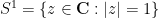${S^1 = \{ z \in {\bf C}: |z|=1 \}}$ . (Usually by abuse of notation we refer to all of these three sets simultaneously as the “unit circle”.) Trigonometric polynomials on the additive unit circle then correspond to ordinary polynomials of the real coefficients ${x,y}$ of the geometric unit circle, or Laurent polynomials of the complex variable ${z}$ .

What about periodic functions on the complex plane? We can start with singly periodic functions ${f: {\bf C} \rightarrow {\bf C}}$ which obey a periodicity relationship ${f(z+\omega)=f(z)}$ for all ${z}$ in the domain and some period ${\omega \in {\bf C} \backslash \{0\}}$ ; such functions can also be viewed as functions on the “additive cylinder” ${\omega {\bf Z} \backslash {\bf C}}$ (or equivalently ${{\bf C} / \omega {\bf Z}}$ ). We can rescale ${\omega=1}$ as before. For holomorphic functions, we have the following characterisations:

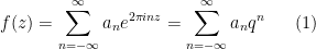
Proposition 1 (Description of singly periodic holomorphic functions)

(i) Every ${1}$ -periodic entire function ${f: {\bf C} \rightarrow {\bf C}}$ has an absolutely convergent expansion
$\displaystyle f(z) = \sum_{n=-\infty}^\infty a_n e^{2\pi i nz} = \sum_{n=-\infty}^\infty a_n q^n \ \ \ \ \ (1)$
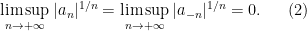
where ${q}$ is the nome ${q := e^{2\pi i z}}$ , and the ${a_n}$ are complex coefficients such that
$\displaystyle \limsup_{n \rightarrow +\infty} |a_n|^{1/n} = \limsup_{n \rightarrow +\infty} |a_{-n}|^{1/n} = 0. \ \ \ \ \ (2)$
Conversely, every doubly infinite sequence ${(a_n)_{n \in {\bf Z}}}$ of coefficients obeying (2) gives rise to a ${1}$ -periodic entire function ${f: {\bf C} \rightarrow {\bf C}}$ via the formula (1).
(ii) Every bounded ${1}$ -periodic holomorphic function ${f: {\bf H} \rightarrow {\bf C}}$ on the upper half-plane ${\{ z: \mathrm{Im}(z) > 0\}}$ has an expansion
$\displaystyle f(z) = \sum_{n=0}^\infty a_n e^{2\pi i nz} = \sum_{n=0}^\infty a_n q^n \ \ \ \ \ (3)$
where the ${a_n}$ are complex coefficients such that
$\displaystyle \limsup_{n \rightarrow +\infty} |a_n|^{1/n} \leq 1. \ \ \ \ \ (4)$
Conversely, every infinite sequence ${(a_n)_{n \in {\bf Z}}}$ obeying (4) gives rise to a ${1}$ -periodic holomorphic function ${f: {\bf H} \rightarrow {\bf C}}$ which is bounded away from the real axis (i.e., bounded on ${\{ z: \mathrm{Im}(z) \geq \varepsilon\}}$ for every ${\varepsilon > 0}$ ).
In both cases, the coefficients ${a_n}$ can be recovered from ${f}$ by the Fourier inversion formula
$\displaystyle a_n = \int_{\gamma_{z_0 \rightarrow z_0+1}} f(z) e^{-2\pi i nz}\ dz \ \ \ \ \ (5)$
for any ${z_0}$ in ${{\bf C}}$ (in case (i)) or ${{\bf H}}$ (in case (ii)).

Proof: If ${f: {\bf C} \rightarrow {\bf C}}$ is ${1}$ -periodic, then it can be expressed as ${f(z) = F(q) = F(e^{2\pi i z})}$ for some function ${F: {\bf C} \backslash \{0\} \rightarrow {\bf C}}$ on the “multiplicative cylinder” ${{\bf C} \backslash \{0\}}$ , since the fibres of the map ${z \mapsto e^{2\pi i z}}$ are cosets of the integers ${{\bf Z}}$ , on which ${f}$ is constant by hypothesis. As the map ${z \mapsto e^{2\pi i z}}$ is a covering map from ${{\bf C}}$ to ${{\bf C} \backslash \{0\}}$ , we see that ${F}$ will be holomorphic if and only if ${f}$ is. Thus ${F}$ must have a Laurent series expansion ${F(q) = \sum_{n=-\infty}^\infty a_n q^n}$ with coefficients ${a_n}$ obeying (2), which gives (1), and the inversion formula (5) follows from the usual contour integration formula for Laurent series coefficients. The converse direction to (i) also follows by reversing the above arguments.

For part (ii), we observe that the map ${z \mapsto e^{2\pi i z}}$ is also a covering map from ${{\bf H}}$ to the punctured disk ${D(0,1) \backslash \{0\}}$ , so we can argue as before except that now ${F}$ is a bounded holomorphic function on the punctured disk. By the Riemann singularity removal theorem (Exercise 35 of 246A Notes 3) ${F}$ extends to be holomorphic on all of ${D(0,1)}$ , and thus has a Taylor expansion ${F(q) = \sum_{n=0}^\infty a_n q^n}$ for some coefficients ${a_n}$ obeying (4). The argument now proceeds as with part (i). $\Box$

The additive cylinder ${{\bf Z} \backslash {\bf C}}$ and the multiplicative cylinder ${{\bf C} \backslash \{0\}}$ can both be identified (on the level of smooth manifolds, at least) with the geometric cylinder ${\{ (x,y,z) \in {\bf R}^3: x^2+y^2=1\}}$ , but we will not use this identification here.

Now let us turn attention to doubly periodic functions of a complex variable ${z}$ , that is to say functions ${f}$ that obey two periodicity relations

$\displaystyle f(z+\omega_1) = f(z); \quad f(z+\omega_2) = f(z)$

for all ${z \in {\bf C}}$ and some periods ${\omega_1,\omega_2 \in {\bf C}}$ , which to avoid degeneracies we will assume to be linearly independent over the reals (thus ${\omega_1,\omega_2}$ are non-zero and the ratio ${\omega_2/\omega_1}$ is not real). One can rescale ${\omega_1,\omega_2}$ by a common scaling factor ${\lambda \in {\bf C} \backslash \{0\}}$ to normalise either ${\omega_1=1}$ or ${\omega_2=1}$ , but one of course cannot simultaneously normalise both parameters in this fashion. As in the singly periodic case, such functions can also be identified with functions on the additive ${2}$ -torus ${\Lambda \backslash {\bf C}}$ , where ${\Lambda}$ is the lattice ${\Lambda := \omega_1 {\bf Z} + \omega_2 {\bf Z}}$ , or with functions ${f}$ on the solid parallelogram bounded by the contour ${\gamma_{0 \rightarrow \omega_1 \rightarrow \omega_1+\omega_2 \rightarrow \omega_2 \rightarrow 0}}$ (a fundamental domain up to boundary for that torus), obeying the boundary periodicity conditions

$\displaystyle f(z+\omega_1) = f(z)$

for ${z}$ in the edge ${\gamma_{\omega_2 \rightarrow 0}}$ , and

$\displaystyle f(z+\omega_2) = f(z)$

for ${z}$ in the edge ${\gamma_{\omega_0 \rightarrow 1}}$ .

Within the world of holomorphic functions, the collection of doubly periodic functions is boring:

Proposition 2 Let ${f: {\bf C} \rightarrow {\bf C}}$ be an entire doubly periodic function (with periods ${\omega_1,\omega_2}$ linearly independent over ${{\bf R}}$ ). Then ${f}$ is constant.

In the language of Riemann surfaces, this proposition asserts that the torus ${\Lambda \backslash {\bf C}}$ is a non-hyperbolic Riemann surface; it cannot be holomorphically mapped non-trivially into a bounded subset of the complex plane.

Proof: The fundamental domain (up to boundary) enclosed by ${\gamma_{0 \rightarrow \omega_1 \rightarrow \omega_1+\omega_2 \rightarrow \omega_2 \rightarrow 0}}$ is compact, hence ${f}$ is bounded on this domain, hence bounded on all of ${{\bf C}}$ by double periodicity. The claim now follows from Liouville’s theorem. (One could alternatively have argued here using the compactness of the torus ${(\omega_1 {\bf Z} + \omega_2 {\bf Z}) \backslash {\bf C}}$ . $\Box$

To obtain more interesting examples of doubly periodic functions, one must therefore turn to the world of meromorphic functions – or equivalently, holomorphic functions into the Riemann sphere ${{\bf C} \cup \{\infty\}}$ . As it turns out, a particularly fundamental example of such a function is the Weierstrass elliptic function

$\displaystyle \wp(z) := \frac{1}{z^2} + \sum_{z_0 \in \Lambda \backslash 0} \left( \frac{1}{(z-z_0)^2} - \frac{1}{z_0^2} \right) \ \ \ \ \ (6)$

which plays a role in doubly periodic functions analogous to the role of ${x \mapsto \cos(2\pi x)}$ for ${1}$ -periodic real functions. This function will have a double pole at the origin ${0}$ , and more generally at all other points on the lattice ${\Lambda}$ , but no other poles. The derivative

$\displaystyle \wp'(z) = -2 \sum_{z_0 \in \Lambda} \frac{1}{(z-z_0)^3} \ \ \ \ \ (7)$

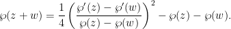
of the Weierstrass function is another doubly periodic meromorphic function, now with a triple pole at every point of ${\Lambda}$ , and plays a role analogous to ${x \mapsto \sin(2\pi x)}$ . Remarkably, all the other doubly periodic meromorphic functions with these periods will turn out to be rational combinations of ${\wp}$ and ${\wp'}$ ; furthermore, in analogy with the identity ${\cos^2 x+ \sin^2 x = 1}$ , one has an identity of the form

$\displaystyle \wp'(z)^2 = 4 \wp(z)^3 - g_2 \wp(z) - g_3 \ \ \ \ \ (8)$

for all ${z \in {\bf C}}$ (avoiding poles) and some complex numbers ${g_2,g_3}$ that depend on the lattice ${\Lambda}$ . Indeed, much as the map ${x \mapsto (\cos 2\pi x, \sin 2\pi x)}$ creates a diffeomorphism between the additive unit circle ${{\bf R}/{\bf Z}}$ to the geometric unit circle ${\{ (x,y) \in{\bf R}^2: x^2+y^2=1\}}$ , the map ${z \mapsto (\wp(z), \wp'(z))}$ turns out to be a complex diffeomorphism between the torus ${(\omega_1 {\bf Z} + \omega_2 {\bf Z}) \backslash {\bf C}}$ and the elliptic curve

$\displaystyle \{ (z, w) \in {\bf C}^2: z^2 = 4w^3 - g_2 w - g_3 \} \cup \{\infty\}$

with the convention that ${(\wp,\wp')}$ maps the origin ${\omega_1 {\bf Z} + \omega_2 {\bf Z}}$ of the torus to the point ${\infty}$ at infinity. (Indeed, one can view elliptic curves as “multiplicative tori”, and both the additive and multiplicative tori can be identified as smooth manifolds with the more familiar geometric torus, but we will not use such an identification here.) This fundamental identification with elliptic curves and tori motivates many of the further remarkable properties of elliptic curves; for instance, the fact that tori are obviously an abelian group gives rise to an abelian group law on elliptic curves (and this law can be interpreted as an analogue of the trigonometric sum identities for ${\wp, \wp'}$ ). The description of the various meromorphic functions on the torus also helps motivate the more general Riemann-Roch theorem that is a fundamental law governing meromorphic functions on other compact Riemann surfaces (and is discussed further in these 246C notes). So far we have focused on studying a single torus ${\Lambda \backslash {\bf C}}$ . However, another important mathematical object of study is the space of all such tori, modulo isomorphism; this is a basic example of a moduli space, known as the (classical, level one) modular curve ${X_0(1)}$ . This curve can be described in a number of ways. On the one hand, it can be viewed as the upper half-plane ${{\bf H} = \{ z: \mathrm{Im}(z) > 0 \}}$ quotiented out by the discrete group ${SL_2({\bf Z})}$ ; on the other hand, by using the ${j}$ -invariant, it can be identified with the complex plane ${{\bf C}}$ ; alternatively, one can compactify the modular curve and identify this compactification with the Riemann sphere ${{\bf C} \cup \{\infty\}}$ . (This identification, by the way, produces a very short proof of the little and great Picard theorems, which we proved in 246A Notes 4.) Functions on the modular curve (such as the ${j}$ -invariant) can be viewed as ${SL_2({\bf Z})}$ -invariant functions on ${{\bf H}}$ , and include the important class of modular functions; they naturally generalise to the larger class of (weakly) modular forms, which are functions on ${{\bf H}}$ which transform in a very specific way under ${SL_2({\bf Z})}$ -action, and which are ubiquitous throughout mathematics, and particularly in number theory. Basic examples of modular forms include the Eisenstein series, which are also the Laurent coefficients of the Weierstrass elliptic functions ${\wp}$ . More number theoretic examples of modular forms include (suitable powers of) theta functions ${\theta}$ , and the modular discriminant ${\Delta}$ . Modular forms are ${1}$ -periodic functions on the half-plane, and hence by Proposition 1 come with Fourier coefficients ${a_n}$ ; these coefficients often turn out to encode a surprising amount of number-theoretic information; a dramatic example of this is the famous modularity theorem, (a special case of which was) used amongst other things to establish Fermat’s last theorem. Modular forms can be generalised to other discrete groups than ${SL_2({\bf Z})}$ (such as congruence groups) and to other domains than the half-plane ${{\bf H}}$ , leading to the important larger class of automorphic forms, which are of major importance in number theory and representation theory, but which are well outside the scope of this course to discuss.

— 1. Doubly periodic functions —

Throughout this section we fix two complex numbers ${\omega_1,\omega_2}$ that are linearly independent over ${{\bf R}}$ , which then generate a lattice ${\Lambda := \omega_1 {\bf Z} + \omega_2{\bf Z}}$ .

We now study the doubly periodic meromorphic functions with respect to these periods that are not identically zero. We first observe some constraints on the poles of these functions. Of course, by periodicity, the poles will themselves be periodic, and thus the set of poles forms a finite union of disjoint cosets ${\zeta_j + \Lambda}$ of the lattice ${\Lambda}$ . Similarly, the zeroes form a finite union of disjoint cosets ${\lambda_j + \Lambda}$ . Using the residue theorem, we can obtain some further constraints:

Lemma 3 (Consequences of residue theorem) Let ${f: {\bf C} \rightarrow {\bf C} \cup \{\infty\}}$ be a doubly periodic meromorphic function (not identically zero) with periods ${\omega_1,\omega_2}$ , poles at ${\zeta_j + \Lambda}$ , and zeroes at ${\lambda_j + \Lambda}$ .

(i) The sum of residues at each ${\zeta_j}$ (i.e., we sum one residue per coset) is equal to zero.
(ii) The number of poles ${\zeta_j}$ (counting multiplicity, but only counting once per coset) is equal to the number of zeroes ${\lambda_j}$ (again counting multiplicity, and once per coset).
(iii) The sum of the poles ${\zeta_j + \Lambda}$ (counting multiplicity, and working in the group ${\Lambda \backslash {\bf C}}$ ) is equal to the sum of the zeroes ${\lambda_j + \Lambda}$ .

Proof: For (i), we first apply a translation so that none of the pole cosets ${\zeta_j + \Lambda}$ intersects the fundamental parallelogram boundary ${\gamma_{0 \rightarrow \omega_1 \rightarrow \omega_1+\omega_2 \rightarrow \omega_2 \rightarrow 0}}$ ; this of course does not affect the sum of residues. Then, by the residue theorem, the sum in (i) is equal to the expression

$\displaystyle \frac{\pm 1}{2\pi i} \int_{\gamma_{0 \rightarrow \omega_1 \rightarrow \omega_1+\omega_2 \rightarrow \omega_2 \rightarrow 0}} f(z)\ dz$

(the sign depends on whether this contour is oriented counter-clockwise or clockwise). But from the double periodicity we see that the integral vanishes (the contribution of parallel pairs of edges cancel each other). For part (ii), apply part (i) to the logarithmic derivative ${f'/f}$ , which is also doubly periodic.

For part (iii), we again translate so that none of the pole or zero cosets intersects ${\gamma_{0 \rightarrow \omega_1 \rightarrow \omega_1+\omega_2 \rightarrow \omega_2 \rightarrow 0}}$ , noting from part (ii) that any such translation affects the sum of poles and sum of zeroes by the same amount. By the residue theorem, it now suffices to show that

$\displaystyle \frac{\pm 1}{2\pi i} \int_{\gamma_{0 \rightarrow \omega_1 \rightarrow \omega_1+\omega_2 \rightarrow \omega_2 \rightarrow 0}} z \frac{f'(z)}{f(z)}\ dz$

lies in the lattice ${\Lambda}$ . But one can rewrite this using the double periodicity as

$\displaystyle \frac{\pm 1}{2\pi i} ( \int_{\gamma_{0 \rightarrow \omega_2}} \omega_1 \frac{f'(z)}{f(z)}\ dz - \int_{\gamma_{0 \rightarrow \omega_1}} \omega_2 \frac{f'(z)}{f(z)}\ dz ),$

so it suffices to show that ${\frac{1}{2\pi i} \int_{\gamma_{0 \rightarrow \omega_j}} \frac{f'(z)}{f(z)}\ dz}$ is an integer for ${j=1,2}$ . But (a slight modification of) the argument principle shows that this number is precisely the winding number around the origin of the image of ${\gamma_{0 \rightarrow \omega_j}}$ under the map ${\frac{f'}{f}}$ , and the claim follows. $\Box$

This lemma severely limits the possible number of behaviors for the zeroes and poles of a meromorphic function. To formalise this, we introduce some general notation:

Definition 4 (Divisors)

(i) A divisor on the torus ${\Lambda\backslash {\bf C}}$ is a formal integer linear combination ${D = \sum_P c_P \cdot (P)}$ , where ${P}$ ranges over a finite collection of points in the torus ${\Lambda \backslash {\bf C}}$ (i.e., a finite collection of cosets ${\zeta + \Lambda}$ ), and ${c_P}$ are integers, with the obvious additive group structure; equivalently, the space ${\mathrm{Div}( \Lambda\backslash {\bf C} )}$ of divisors is the free abelian group with generators ${(P)}$ for ${P \in \Lambda \backslash {\bf C}}$ (with the convention ${1 \cdot (P) = (P)}$ ).
(ii) The number ${\sum_P c_P}$ is the degree ${\mathrm{deg}(D)}$ of a divisor ${D = \sum_P c_P \cdot (P)}$ , the point ${\sum_P c_P P \in \Lambda \backslash {\bf C}}$ is the sum ${\mathrm{sum}(D)}$ of ${D}$ , and each ${c_P}$ is the order ${\mathrm{ord}_P(D)}$ of the divisor at ${P}$ (with the convention that the order is ${0}$ if ${P}$ does not appear in the sum). A divisor is non-negative (or effective) if ${c_P \geq 0}$ for all ${P}$ . We write ${D_1 \geq D_2}$ if ${D_1 - D_2}$ is non-negative (i.e., the order of ${D_1}$ is greater than or equal to that of ${D_2}$ at every point ${P}$ , and ${D_1 > D_2}$ if ${D_1 \geq D_2}$ and ${D_1 \neq D_2}$ .
(iii) Given a meromorphic function ${f: \Lambda \backslash {\bf C} \rightarrow {\bf C} \cup \{\infty\}}$ (or equivalently, a doubly periodic function ${f: {\bf C} \rightarrow {\bf C} \cup \{\infty\}}$ ) that is not identically zero, the principal divisor ${(f)}$ is the divisor ${\sum_P \mathrm{ord}_P(f) (P)}$ , where ${P}$ ranges over the zeroes and poles of ${f}$ , and ${\mathrm{ord}_P(f)}$ is the order of the zero (if ${P}$ is a zero) or negative the order of the pole (if ${P}$ is a pole).
(iv) Given a divisor ${D = \sum_P c_P \cdot (P)}$ , we define ${L(D)}$ to be the space of all meromorphic functions ${f}$ that are either zero, or are such that ${(f)+D \geq 0}$ . That is to say, ${L(D)}$ consists of those meromorphic functions that have at most a pole of order ${c_P}$ at ${P}$ if ${c_P}$ is positive, or at least zero of order ${-c_P}$ if ${c_P}$ is negative.

A divisor can be viewed as an abstraction of the concept of a set of zeroes and poles (counting multiplicity). Observe that principal divisors obey the laws ${(fg) = (f)+(g)}$ , ${(f/g) = (f) - (g)}$ when ${f,g}$ are meromorphic and non-zero. In particular, the space ${\mathrm{PDiv}(\Lambda \backslash {\bf C})}$ of principal divisors is a subgroup of the space ${\mathrm{Div}(\Lambda \backslash {\bf C})}$ of all divisors. By Lemma 3(ii), all principal divisors have degree zero, and from Lemma 3(iii), all principal divisors have sum zero as well. Later on we shall establish the converse claim that every divisor of degree and sum zero is a principal divisor; see Exercise 7.

Remark 5 One can define divisors on other Riemann surfaces, such as the complex plane ${{\bf C}}$ . Observe from the fundamental theorem of algebra that if one has two non-zero polynomials ${P(z), Q(z)}$ , then ${(P) \leq (Q)}$ if and only if ${P}$ divides ${Q}$ as a polynomial. This may give some hint as to the origin of the terminology “divisor”. The machinery of divisors turns out to have a rich algebraic and topological structure when applied to more general Riemann surfaces than tori, for instance enabling one to associate an abelian variety (the Jacobian variety) to every algebraic curve; see these 246C notes for further discussion.

It is easy to see that ${L(D)}$ is always a vector space. All non-zero meromorphic functions ${f: \Lambda \backslash {\bf C} \rightarrow {\bf C}}$ belong to at least one of the ${L(D)}$ , namely ${L(-(f))}$ , so to classify all the meromorphic functions on ${\Lambda \backslash {\bf C}}$ , it would suffice to understand what all the spaces ${L(D)}$ are.

Liouville’s theorem (in the form of Proposition 2) tells us that all elements of ${L(0)}$ – that is to say, the holomorphic functions on ${\Lambda \backslash {\bf C}}$ – are constant; thus ${L(0)}$ is one-dimensional. If ${D<0}$ is a negative divisor, the elements of ${L(D)}$ are thus constant and have at least one zero, thus in these cases ${L(D)}$ is trivial.

Now we gradually work our way up to higher degree divisors ${L(D)}$ . A basic fact, proven from elementary linear algebra, is that every time one adds a pole to ${D}$ , the dimension of the space ${L(D)}$ only goes up by at most one:

Lemma 6 For any divisor ${D}$ and any ${P \in \Lambda \backslash {\bf C}}$ , ${L(D)}$ is a subspace of ${L(D + (P))}$ of codimension at most one. In particular, ${L(D)}$ is finite-dimensional for any ${D}$ .

Proof: It is clear that ${L(D)}$ is a subspace of ${L(D + (P))}$ . If ${D}$ has order ${m}$ at ${P = \zeta + \Lambda}$ , then there is a linear functional ${\lambda: L(D+(P)) \rightarrow {\bf C}}$ that assigns to each meromorphic function ${f: \Lambda \backslash {\bf C} \rightarrow {\bf C} \cup \{\infty\}}$ the ${\frac{1}{(z-\zeta)^{m+1}}}$ coefficient of the Laurent expansion of ${f}$ at ${\zeta}$ (note from periodicity that the exact choice of coset representative ${\zeta}$ is not relevant. A little thought reveals that the kernel of ${\lambda}$ is precisely ${L(D)}$ , and the first claim follows. The second claim follows from iterating the first claim, noting that any divisor ${D}$ can be obtained from a suitable negative divisor by the addition of finitely many poles ${(P)}$ . $\Box$

Now consider the space ${L((P))}$ for some point ${P \in \Lambda \backslash {\bf C}}$ . Lemma 6 tells us that the dimension of this space is either one or two, since ${L(0)}$ was one-dimensional. The space ${L((P))}$ consists of functions ${f}$ that possibly have a simple pole at most at ${P}$ , and no other poles. But Lemma 3(i) tells us that the residue at ${P}$ has to vanish, and so ${f}$ is in fact in ${L(0)}$ and thus is constant. (One could also argue here using the other two parts of Lemma 2; how?) So ${L((P))}$ is no larger than ${L(0)}$ , and is thus also one-dimensional.

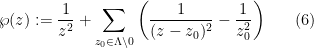
Now let us study the space ${L(2 \cdot (P))}$ – the space of meromorphic functions that have at most a double pole at ${P}$ and no other poles. Again, Lemma 6 tells us that this space is one or two dimensional. To figure out which, we can normalise ${P}$ to be the origin coset ${\Lambda}$ . The question is now whether there is a doubly periodic meromorphic function that has a double pole at each point of ${\Lambda}$ . A naive candidate for such a function would be the infinite series

$\displaystyle \sum_{z_0 \in \Lambda} \frac{1}{(z-z_0)^2},$

however this series turns out to not be absolutely convergent. Somewhat in analogy with the discussion of the Weierstrass and Hadamard factorisation theorems in Notes 1, we then proceed instead by working with the normalised function ${\wp}$ defined by the formula (6). Let us first verify that the series in (6) is absolutely convergent for ${z \not \in \Lambda}$ . There are only finitely many ${z_0 \in \Lambda}$ with ${|z_0| \leq 2|z|}$ , and all the summands are finite for ${z \not \in\Lambda}$ , so we only need to establish convergence of the tail

$\displaystyle \sum_{z_0 \in \Lambda: |z_0| \geq 2|z|} \frac{1}{(z-z_0)^2} - \frac{1}{z_0^2}.$

However, from the fundamental theorem of calculus we have

$\displaystyle \frac{1}{(z-z_0)^2} - \frac{1}{z_0^2} = z\int_0^1 \frac{-2}{(tz-z_0)^3}\ dt = O_z( |z_0|^{-3} )$

so to demonstrate absolute convergence it suffices to show that

$\displaystyle \sum_{z_0 \in \Lambda: z_0 \neq 0} \frac{1}{|z_0|^3} < \infty.$

But a simple volume packing argument (considering the areas of the translates ${z_0 + D}$ of the fundamental domain ${D}$ ) shows that the number of lattice points ${z_0}$ in any disk ${D(0,R)}$ , ${R \geq 1}$ is ${O_\Lambda(R^2)}$ , and so by dyadic decomposition as in Notes 1, the series is absolutely convergent. Further repetition of the arguments from Notes 1 shows that the series in (6) converges locally uniformly in ${{\bf C} \backslash \Lambda}$ , and thus is holomorphic on this set. Furthermore, for any ${z_0 \in \Lambda}$ , the same arguments show that ${\wp(z) - \frac{1}{(z-z_0)^2}}$ stays bounded in a punctured neighbourhood of ${z_0}$ , thus by the Riemann singularity removal theorem ${\wp(z)}$ is equal to ${\frac{1}{(z-z_0)^2}}$ plus a bounded holomorphic function in the neighbourhood of ${z_0}$ . Thus ${\wp}$ is meromorphic with double poles (and vanishing residue) at every lattice point ${\Lambda}$ , and no other poles.

Now we show that ${\wp}$ is doubly periodic, thus ${\wp(z + \omega_1) = \wp(z)}$ and ${\wp(z + \omega_2) = \wp(z)}$ for ${z \in {\bf C} \backslash \Lambda}$ . We just prove the first identity, as the second is analogous. From (6) we have

$\displaystyle \wp(z+\omega_1) - \wp(z) = \sum_{z_0 \in \Lambda} \frac{1}{(z-z_0+\omega_1)^2} - \frac{1}{(z-z_0)^2}.$

The series on the right is absolutely convergent, and on every coset of ${\omega_1 {\bf Z}}$ it telescopes to zero. The claim then follows by Fubini’s theorem.

By construction, ${\wp}$ lies in ${L(2 \cdot (\Lambda))}$ , and is clearly non-constant. Thus ${L(2 \cdot (\Lambda))}$ is two-dimensional, being spanned by the constant function ${1}$ and ${\wp}$ . By translation, we see that ${L(2 \cdot (P))}$ is two-dimensional for any other point ${P \in \Lambda \backslash {\bf C}}$ as well.

From (6) it is also clear that the function ${\wp}$ is even: ${\wp(-z) = \wp(z)}$ . In particular, for any ${a \in {\bf C}}$ avoiding the half-lattice ${\frac{1}{2} \Lambda = \{ \frac{1}{2} z_0: z_0 \in \Lambda\}}$ (so that ${a}$ and ${-a}$ occupy different locations in the torus ${\Lambda \backslash {\bf C}}$ ), the function ${\wp - \wp(a) \in L(2 \cdot (\Lambda))}$ has a zero at both ${a+\Lambda}$ and ${-a+\Lambda}$ . By Lemma 3(ii) there are no other zeroes of this function (and this claim is also consistent with Lemma 3(iii)); thus the divisor ${(\wp - \wp(a))}$ of this function is given by

$\displaystyle (\wp - \wp(a)) = -2 \cdot (\Lambda) + (a + \Lambda) + (-a+\Lambda). \ \ \ \ \ (9)$

If ${a}$ lies in the half-lattice ${\frac{1}{2} \Lambda}$ but not in ${\Lambda}$ (thus, it lies in one of the half-periods ${\frac{\omega_1}{2} + \Lambda}$ , ${\frac{\omega_2}{2} + \Lambda}$ , or ${\frac{\omega_1+\omega_2}{2} + \Lambda}$ ) then from the even and doubly periodic nature of ${\wp}$ we see that ${\wp(a+z) = \wp(a-z)}$ for all ${z \not \in \frac{1}{2} \Lambda}$ , so ${\wp - \wp(a)}$ in fact must have at least a double zero at ${a}$ , and again from Lemma 3(ii) these are the only zeroes of this function. So the identity (9) also holds in this case.

Exercise 7 (Classification of principal divisors)

(i) Let ${P,Q,R,S}$ be four points ${\Lambda \backslash {\bf C}}$ such that ${P+Q=R+S}$ . Show that the divisor ${(P)+(Q)-(R)-(S)}$ is a principal divisor. (Hint: if ${P = \zeta_P + \Lambda, Q = \zeta_Q + \Lambda, R = \zeta_R + \Lambda, S = \zeta_S + \Lambda}$ are all distinct, use a function such as
$\displaystyle f(z) := \sum_{z_0 \in \Lambda} \frac{1}{z-(\zeta_R+z_0)} - \frac{1}{z-(\zeta_S+z_0)}$

$\displaystyle - \frac{1}{\zeta_P-(\zeta_R+z_0)} + \frac{1}{\zeta_P-(\zeta_S+z_0)} .$
If some of the ${P,Q,R,S}$ coincide, use some transformed version of the Weierstrass elliptic function ${\wp}$ instead.)
(ii) Show that every divisor of degree zero and sum zero is a principal divisor.
(iii) Two divisors are said to be equivalent if their difference is a principal divisor. Show that two divisors are equivalent if and only if they have the same degree and same sum.
(iv) Show that the quotient group ${\mathrm{Pic}(\Lambda \backslash {\bf C}) := \mathrm{Div}(\Lambda \backslash {\bf C}) / \mathrm{PDiv}(\Lambda \backslash {\bf C})}$ (known as the divisor class group or Picard group) is isomorphic (as a group) to ${{\bf Z} \times (\Lambda \backslash {\bf C})}$ , and that the subgroup ${\mathrm{Pic}^0(\Lambda \backslash {\bf C})}$ arising from degree zero divisors (also known as the Jacobian variety of ${\Lambda \backslash {\bf C}}$ ) is isomorphic to ${\Lambda \backslash {\bf C}}$ .

Now let us study the space ${L(3 \cdot (P))}$ , where we again normalise ${P = \Lambda}$ for sake of discussion. Lemma 6 tells us that this space is two or three dimensional, being spanned by ${1}$ , ${\wp}$ , and possibly one other function. Note that the derivative ${\wp'}$ of the meromorphic function ${\wp}$ is also doubly periodic with a triple pole at ${P}$ , so it lies in ${L(3 \cdot (P))}$ and is not a linear combination of ${1}$ or ${\wp}$ (as these have a lower order singularity at ${P}$ ). Thus ${L(3 \cdot (\Lambda))}$ is three-dimensional, being spanned by ${1,\wp,\wp'}$ . A formal term-by-term differentiation of (6) gives (7). To justify (7), observe that the arguments that demonstrated the meromorphicity of the right-hand side of (6) also show the meromorphicity of (7). From Fubini’s theorem, the fundamental theorem of calculus, and (6) we see that

$\displaystyle \int_\gamma (-2 \sum_{z_0 \in \Lambda} \frac{1}{(z-z_0)^3})\ dz = \wp(z_2) - \wp(z_1)$

for any contour ${\gamma}$ in ${{\bf C} \backslash \Lambda}$ from one point ${z_1 \in {\bf C} \backslash \Lambda}$ to another ${z_2 \in {\bf C} \backslash \Lambda}$ , and the claim (7) now follows from another appeal to the fundamental theorem of calculus. Of course, ${L(3 \cdot (P))}$ will then also be three-dimensional for any other point ${P}$ on the torus. From (7) we also see that ${\wp'}$ is odd; this also follows from the even nature of ${\wp}$ . From the oddness and periodicity ${\wp'}$ has to have zeroes at the half-periods ${\frac{1}{2} \Lambda \backslash \Lambda}$ ; in particular, from Lemma 3(ii) there are no other zeroes, and the principal divisor is given by

$\displaystyle (\wp') = -3 \cdot (\Lambda) + (\frac{\omega_1}{2} + \Lambda) + (\frac{\omega_2}{2}+\Lambda) + (\frac{\omega_1+\omega_2}{2}+\Lambda). \ \ \ \ \ (10)$

Turning now to ${L(4 \cdot (\Lambda))}$ , we could differentiate ${\wp}$ yet again to generate a doubly periodic function ${\wp''}$ with a fourth order pole at the origin, but we can also work with the square ${\wp^2}$ of the Weierstrass function. From Lemma 6 we conclude that ${L(4 \cdot (\Lambda))}$ is four-dimensional and is spanned by ${1, \wp, \wp^2, \wp'}$ . In a similar fashion, ${L(5 \cdot (\Lambda))}$ is a five-dimensional space spanned by ${1, \wp, \wp^2, \wp', \wp \wp'}$ .

Something interesting happens though at ${L(6 \cdot (\Lambda))}$ . Lemma 6 tells us that this space is the span of ${1, \wp, \wp^2, \wp', \wp\wp'}$ , and possibly one other function, which will have a pole of order six at the origin. Here we have two natural candidates for such a function: the cube ${\wp^3}$ of the Weierstrass function, and the square ${(\wp')^2}$ of its derivative. Both have a pole of order exactly six and lie in ${L(6 \cdot (\Lambda))}$ , and so ${(\wp')^2}$ must be a linear combination of ${1, \wp, \wp^2, \wp^3, \wp', \wp \wp'}$ . But since ${(\wp')^2, 1, \wp, \wp^2, \wp^3}$ are even and ${\wp', \wp \wp'}$ are odd, ${(\wp')^2}$ must in fact just be a linear combination of ${1, \wp, \wp^2, \wp^3}$ . To work out the precise combination, we see by repeating the derivation of (7) that

$\displaystyle \wp^{(k)}(z) = (-1)^k (k+1)! \sum_{z_0 \in \Lambda} \frac{1}{(z-z_0)^{k+2}}$

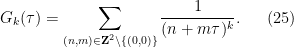
for any ${k=1,2,\dots}$ , so that the function ${\wp(z) - \frac{1}{z^2}}$ , which extends holomorphically to the origin, has ${k^{th}}$ derivative at the origin equal to 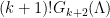${(k+1)! G_{k+2}(\Lambda)}$ , where the Eisenstein series ${G_k(\Lambda)}$ is defined by the formula

$\displaystyle G_k(\Lambda) := \sum_{z_0 \in \Lambda \backslash \{0\}} \frac{1}{z_0^k};$

we can also extend this to the ${k=0}$ case with convention ${G_2(\Lambda)=0}$ . Note from the symmetric nature of ${\Lambda}$ that ${G_k(\Lambda)}$ vanishes for odd ${k}$ ; this is consistent with the even nature of ${\wp}$ . We thus have the Laurent expansion

$\displaystyle \wp(z) = \frac{1}{z^2} + \sum_{k=1}^\infty (2k+1) G_{2k+2}(\Lambda) z^{2k}$

$\displaystyle = \frac{1}{z^2} + 3 G_4(\Lambda) z^2 + 5 G_6(\Lambda) z^4 + \dots$

for ${z}$ near zero. This then gives the further Laurent expansions

$\displaystyle \wp(z)^2 = \frac{1}{z^4} + 6 G_4(\Lambda) + 10 G_6(\Lambda) z^2 + \dots$

$\displaystyle \wp(z)^3 = \frac{1}{z^6} + \frac{9 G_4(\Lambda)}{z^2} + 15 G_6(\Lambda) + \dots$

$\displaystyle \wp'(z) = -\frac{2}{z^3} + 6 G_4(\Lambda) z + 20 G_6(\Lambda) z^3 + \dots$

$\displaystyle \wp'(z)^2 = \frac{4}{z^6} - \frac{24 G_4(\Lambda)}{z^2} - 80 G_6(\Lambda) + \dots.$

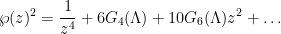
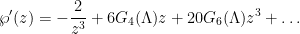
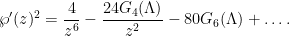
From these expansions we see that the decomposition of ${\wp'(z)^2}$ into a linear combination of ${1,\wp,\wp^2,\wp^3}$ does not actually involve ${\wp^2}$ (as this function is the only one that has a ${1/z^4}$ term in its Laurent expansion), and on comparing ${1/z^6}$ coefficients we see that the coefficient of ${\wp^3}$ must be ${4}$ . Thus we have a linear relationship of the form (8) for some coefficients ${g_2 = g_2(\Lambda), g_3 = g_3(\Lambda)}$ , which on inspection of the ${\frac{1}{z^2}}$ and constant terms leads to the formulae

$\displaystyle g_2 := 60 G_4(\Lambda); \quad g_3 := 140 G_6(\Lambda).$

Exercise 8 Derive (8) directly from Proposition 2 by showing that the difference between the two sides is doubly periodic and holomorphic after removing singularities.

Exercise 9 (Classification of doubly periodic meromorphic functions)

(i) For any ${k \geq 2}$ , show that ${L( k \cdot (\Lambda))}$ has dimension ${k}$ , and every element of this space is a polynomial combination of ${\wp, \wp'}$ .
(ii) Show that every doubly periodic meromorphic function is a rational function of ${\wp, \wp'}$ .

We have an alternate form of (8):

Exercise 10 Define the roots ${e_1 := \wp( \frac{\omega_1}{2} )}$ , ${e_2 := \wp( \frac{\omega_2}{2} )}$ , ${e_3 := \wp( \frac{\omega_1+\omega_2}{2} )}$ .

(i) Show that ${e_1,e_2,e_3}$ are distinct, and that
$\displaystyle (\wp'(z))^2 = 4 (\wp(z) - e_1) (\wp(z) - e_2) (\wp(z) - e_3)$
for all ${z \in {\bf C} \backslash \Lambda}$ . (Hint: use (10).) Conclude in particular that ${e_1+e_2+e_3=0}$ , ${g_2 = 2(e_1^2+e_2^2+e_3^2)}$ , and ${g_3=4e_1e_2e_3}$ .
(ii) Show that the modular discriminant
$\displaystyle \Delta = \Delta(\Lambda) := g_2^3 - 27 g_3^2$
is equal to ${16(e_1-e_2)^2 (e_2-e_3)^2 (e_1-e_3)^2}$ , and is in particular non-zero.

If we now define the elliptic curve

$\displaystyle C := \{ (z,w) \in {\bf C}^2: w^2 = 4z^3 - g_2 z - g_3 \} \cup \{ \infty\}$

$\displaystyle = \{ (z,w) \in {\bf C}^2: w^2 = 4(z-e_1)(z-e_2)(z-e_3) \} \cup \{ \infty\}$

to be the union of a certain cubic curve in the complex plane ${{\bf C}^2}$ together with the point at infinity (where the notions of “curve” and “plane” are relative to the underlying complex field ${{\bf C}}$ rather than the more familiar real field ${{\bf R}}$ ), then we have a map

$\displaystyle \Phi: z \mapsto (\wp(z), \wp'(z)) \ \ \ \ \ (11)$

from ${\Lambda \backslash {\bf C}}$ to ${C}$ , with the convention that the origin ${\Lambda}$ is mapped to the point at infinity ${\infty}$ . For instance, the half-periods ${\frac{\omega_1}{2} + \Lambda}$ , ${\frac{\omega_2}{2} + \Lambda}$ , ${\frac{\omega_1+\omega_2}{2} + \Lambda}$ are mapped to the points ${(e_1,0), (e_2,0), (e_3,0)}$ of ${C}$ respectively.

Lemma 11 The map ${\Phi}$ defined by (11) is a bijection between ${\Lambda \backslash {\bf C}}$ and ${C}$ .

Among other things, this lemma implies that the elliptic curve ${C}$ is topologically equivalent (i.e., homeomorphic to) a torus, which is not an entirely obvious fact (though if one squints hard enough, the real analogue of an elliptic curve does resemble a distorted slice of a torus embedded in ${{\bf R}^3}$ ).

Proof: Clearly ${\Lambda}$ is the only point that maps to ${\infty}$ , and (from (10)) the half-periods are the only points that map to ${(e_1,0), (e_2,0), (e_3,0)}$ . It remains to show that all the other points ${(z,w)}$ arise via ${\Phi}$ from exactly one element of ${\Lambda \backslash {\bf C}}$ . The function ${\wp - z}$ has exactly two zeroes by Lemma 3(ii), which lie at ${a+\Lambda, -a+\Lambda}$ for some ${a}$ as ${\wp}$ is even; since ${(z,w) \neq (e_1,0), (e_2,0), (e_3,0)}$ , ${z}$ is not equal to ${e_1,e_2,e_3}$ , hence ${a}$ is not a half-period. As ${\wp'}$ is odd, the map (11) must therefore map ${a+\Lambda, -a+\Lambda}$ to the two points ${(z,w), (z,-w)}$ of the elliptic curve ${C}$ that lie above ${z}$ , and the claim follows. $\Box$

Analogously to the Riemann sphere ${{\bf C} \cup \{ \infty\}}$ , the elliptic curve ${C}$ can be given the structure of a Riemann surface, by prescribing the following charts:

(i) When ${(z_0,w_0)}$ is a point in ${C}$ other than ${\infty}$ or ${(e_1,0), (e_2,0), (e_3,0)}$ , then locally ${C}$ is the graph of a holomorphic branch ${(4(z-e_1)(z-e_2)(z-e_3))^{1/2}}$ of the square root of ${4(z-e_1)(z-e_2)(z-e_3)}$ near ${(z_0,w_0)}$ , and one can use ${z}$ as a coordinate function in a sufficiently small neighbourhood of ${(z_0,w_0)}$ .
(ii) In the neighbourhood of ${(e_j,0)}$ for some ${j=1,2,3}$ , the function ${f: z \mapsto 4(z-e_1)(z-e_2)(z-e_3)}$ has a simple zero at ${e_j}$ and so has a local inverse ${f^{-1}}$ that maps a neighbourhood of ${0}$ to a neighbourhood of ${e_j}$ , and a point ${(z,w)}$ sufficiently near ${(e_j,0)}$ can be parameterised by ${(f^{-1}(w^2),w)}$ . One can then use ${w}$ as a coordinate function in a neighbourhood of ${(e_j,0)}$ .
(iii) A neighbourhood of ${\infty}$ consists of ${\infty}$ and the points ${(z,w)}$ in the remaining portion of ${C}$ with ${z, w}$ sufficiently large; then ${w}$ is asymptotic to a square root of ${4z^3}$ , so in particular ${w/z^2}$ and ${1/z}$ should both go to zero as ${(z,w)}$ goes to infinity in ${C}$ . We rewrite the defining equation ${w^2 = 4z^3 - g_2 z - g_3}$ of the curve in terms of ${w/z^2}$ and ${1/z}$ as ${(w/z^2)^2 = 4 (1/z) - g_2 (1/z)^3 - g_3 (1/z)^4}$ . The function ${h(\xi) := 4 \xi - g_2 \xi^3 - g_3 \xi^4}$ has a simple zero at zero and thus has a holomorphic local inverse ${h^{-1}}$ that maps ${0}$ to ${0}$ , and we have ${1/z = h^{-1}((w/z^2)^2)}$ in a neighbourhood of infinity. We can then use ${w/z^2}$ as a coordinate function in a neighbourhood of ${\infty}$ , with the convention that this coordinate function vanishes at infinity.

It is then a tedious but routine matter to check that ${C}$ has the structure of a Riemann surface. We then claim that the bijection ${\Phi}$ defined by (11) is holomorphic, and thus a complex diffeomorphism of Riemann surfaces. In the neighbourhood of any point ${\zeta+\Lambda}$ of the torus ${\Lambda \backslash {\bf C}}$ other than the origin ${\Lambda}$ , ${\Phi}$ maps to a neighbourhood of finite point ${(z,w)}$ of ${C}$ , including the three points ${(e_1,0), (e_2,0), (e_3,0)}$ , the holomorphicity is a routine consequence of composing together the various local holomorphic functions and their inverses. In the neighbourhood of the origin ${\Lambda}$ , ${\Phi}$ maps ${z+\Lambda}$ for small ${z}$ to a point of ${C}$ with a Laurent expansion

$\displaystyle (\frac{1}{z^2} + O(z^2), \frac{-2}{z^3} + O(z))$

from the Laurent expansions of ${\wp, \wp'}$ , so in particular the coordinate ${w/z^2}$ takes the form ${-4 z + O(z^5)}$ where the error term ${O(z^5)}$ is holomorphic, with ${0}$ mapping to ${0}$ . In particular the map is a local complex diffeomorphism here and again we have holomorphicity. We thus conclude that the elliptic curve ${C}$ is complex diffeomorphic to the torus ${\Lambda \backslash {\bf C}}$ using the map ${\Phi}$ . From Exercise 9, the meromorphic functions on ${\Lambda \backslash {\bf C}}$ may be identified with the rational functions on ${C}$ .

While we have shown that all tori are complex diffeomorphic to elliptic curves, the converse statement that all elliptic curves are diffeomorphic to tori will have to wait until the next section for a proof, once we have set up the machinery of modular forms.

Exercise 12 (Group law on elliptic curves)

(i) Let ${P,Q,R}$ be three distinct elements of the torus ${\Lambda \backslash {\bf C}}$ that are not equal to the origin ${\Lambda}$ . Show that ${P+Q+R=\Lambda}$ if and only if the three points ${(\wp(P), \wp'(P))}$ , ${(\wp(Q), \wp'(Q))}$ , ${(\wp(R), \wp'(R))}$ are collinear in ${C}$ , in the sense that they lie on a common complex line ${\{ (z,w) \in {\bf C}^2: az+bw=c\}}$ for some complex numbers ${a,b,c}$ with ${a,b}$ not both zero.
(ii) What happens in (i) if (say) ${P}$ and ${Q}$ agree? What about if ${R = \Lambda}$ ?
(iii) Using (i), (ii), give a purely geometric definition of a group addition law on the elliptic curve ${C}$ which is compatible with the group addition law on the torus ${\Lambda \backslash {\bf C}}$ via (11). (We remark that the associativity property of this law is not obvious from a purely geometric perspective, and is related to the Cayley-Bacharach theorem in classical geometry; see this previous blog post.)

Exercise 13 (Addition law) Show that for any ${z, w \in {\bf C} \backslash \Lambda}$ with ${z-w, z+w \not \in \Lambda}$ , one has
$\displaystyle \wp(z+w) = \frac{1}{4} \left( \frac{\wp'(z) - \wp'(w)}{\wp(z)-\wp(w)} \right)^2 - \wp(z) - \wp(w).$

Exercise 14 (Special case of Riemann-Roch)

(i) Show that if two divisors ${D,D'}$ are equivalent (in the sense of Exercise 7(iii)), then the vector spaces ${L(D)}$ and ${L(D')}$ are isomorphic (in particular, they have the same dimension).
(ii) If ${D}$ is a divisor of some degree ${d}$ , show that the dimension of the space ${L(D)}$ is zero if ${d < 0}$ , equal to ${d}$ if ${d>0}$ , equal to ${0}$ if ${d=0}$ and ${D}$ has non-zero sum, and equal to ${1}$ if ${d=0}$ and ${D}$ has zero sum. (Hint: use Exercise 7(iii) and part (i) to replace ${D}$ with an equivalent divisor of a simple form.)
(iii) Verify the identity
$\displaystyle \mathrm{dim} L(D) - \mathrm{dim} L(-D) = \mathrm{deg}(D)$
for any divisor ${D}$ . This is a special case of the more general Riemann-Roch theorem, discussed in these 246C notes.

Exercise 15 (Elliptic integrals)

(i) Show that ${\wp}$ is a covering map from ${{\bf C} \backslash \frac{1}{2} \Lambda}$ to the thrice-punctured plane ${{\bf C} \backslash \{e_1,e_2,e_3\}}$ .
(ii) Let ${\gamma}$ be a contour in ${{\bf C} \backslash \{e_1,e_2,e_3\}}$ from some complex number ${z_1}$ to another complex number ${z_2}$ , and suppose that there is a holomorphic branch ${\sqrt{4(z-e_1)(z-e_2)(z-e_3)}}$ of the square root of ${4(z-e_1)(z-e_2)(z-e_3)}$ in a neighbourhood of ${\gamma}$ . Show that there exists complex numbers ${\zeta_1, \zeta_2 \in {\bf C} \backslash \frac{1}{2} \Lambda}$ with ${\wp(\zeta_1) = z_1}$ , ${\wp(\zeta_2) = z_2}$ such that
$\displaystyle \int_\gamma \frac{dz}{\sqrt{4(z-e_1)(z-e_2)(z-e_3)}} = \zeta_2 - \zeta_1. \ \ \ \ \ (12)$

Remark 16 The integral ${\int_\gamma \frac{dz}{\sqrt{4(z-e_1)(z-e_2)(z-e_3)}}}$ is an example of an elliptic integral; many other elliptic integrals (such as the integral arising when computing the perimeter of an ellipse) can be transformed into this form (or into a closely related integral) by various elementary substitutions. Thus the Weierstrass elliptic function ${\wp}$ can be employed to evaluate elliptic integrals, which may help explain the terminology “elliptic” that occurs throughout these notes. In 246C notes we will introduce the notion of a meromorphic ${1}$ -form on a Riemann surface. The identity (12) can then be interpreted in this language as the differential form identity ${d(\Phi^{-1}) = \frac{dz}{w}}$ , where ${z,w}$ are the standard coordinates on the elliptic curve ${C}$ ; the meromorphic ${1}$ -form is initially only defined on ${C}$ outside of the four points ${(e_1,0), (e_2,0), (e_3,0), \infty}$ , but this identity in fact reveals that the form extends holomorphically to all of ${C}$ ; it is an example of what is known as an Abelian differential of the first kind.

Remark 17 The elliptic curve ${C}$ (for various choices of parameters ${g_2,g_3}$ ) can be defined in other fields than the complex numbers (though some technicalities arise in characteristic two and three due to the pathological behaviour of the discriminant in those cases). On the other hand, the Weierstrass elliptic function ${\wp}$ is a transcendental function which only exists in complex analysis and does not have a direct analogue in other fields. So this connection between elliptic curves and tori is specific to the complex field. Nevertheless, many facts about elliptic curves that were initially discovered over the complex numbers through this complex-analytic link to tori, were then reproven by purely algebraic means, so that they could be extended without much difficulty to many other fields than the complex numbers, such as finite fields. (For instance, the role of the complex torus can be replaced by the Jacobian variety, which was briefly introduced in Exercise 7.) Elliptic curves over such fields are of major importance in number theory (and cryptography), but we will not discuss these topics further here.

— 2. Modular functions and modular forms —

In Exercise 32 of 246A Notes 5, it was shown that two tori ${(\omega_1 {\bf Z} + \omega_2{\bf Z}) \backslash {\bf C}}$ and ${(\omega'_1 {\bf Z} + \omega'_2{\bf Z}) \backslash {\bf C}}$ are complex diffeomorphic if and only if one has

$\displaystyle \frac{\omega'_1}{\omega'_2} = \pm \frac{a\omega_1+b\omega_2}{c\omega_1+d\omega_2} \ \ \ \ \ (13)$

for some integers ${a,b,c,d}$ with ${ad-bc=1}$ . From this it is not difficult to see that if ${\Lambda,\Lambda'}$ are two lattices in ${{\bf C}}$ , then ${\Lambda \backslash {\bf C}}$ and ${\Lambda' \backslash {\bf C}}$ are diffeomorphic if and only if ${\Lambda' = \lambda \cdot \Lambda}$ for some ${\lambda \in {\bf C} \backslash \{0\}}$ , i.e., the lattices ${\Lambda,\Lambda'}$ are complex dilations of each other.

Let us write ${X_0(1)}$ for the set of all tori ${\Lambda \backslash {\bf C}}$ quotiented by the equivalence relation of complex diffeomorphism; this is the (classical, level one, noncompactified) modular curve. By the above discussion, this set can also be identified with the set of pairs ${(\omega_1,\omega_2)}$ of linearly independent (over ${{\bf R}}$ ) complex numbers quotiented by the equivalence relation given implicitly by (13). One can simplify this a little by observing that any pair ${(\omega_1,\omega_2)}$ is equivalent to ${(1,\tau)}$ for some ${\tau}$ in the upper half-plane ${{\mathbf H}}$ , namely either ${+\omega_2/\omega_1}$ or ${-\omega_2/\omega_1}$ depending on the relative phases of ${\omega_1}$ and ${\omega_2}$ ; this quantity ${\tau}$ is known as the period ratio. From (13) (swapping the roles of ${\omega_1,\omega_2}$ as necessary), we then see that two pairs ${(1,\tau), (1,\tau')}$ are equivalent if one has

$\displaystyle \tau' = \pm \frac{a \tau + b}{c\tau + d}$

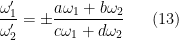
for some integers ${a,b,c,d}$ with ${ad-bc=1}$ . Recall that the Möbius transformation ${\tau \mapsto \frac{a \tau + b}{c\tau + d}}$ preserves ${{\bf H}}$ (see Exercise 20 of 246A Notes 5), so the ${\pm}$ sign here must actually be positive. We can interpret this in terms of the action of the matrix group

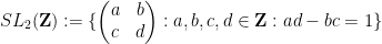$\displaystyle SL_2({\bf Z}) := \{ \begin{pmatrix} a & b \\ c & d \end{pmatrix}: a,b,c,d \in {\bf Z}: ad-bc = 1 \}$

on ${{\bf H}}$ by Möbius transformation

$\displaystyle \begin{pmatrix} a & b \\ c & d \end{pmatrix} \cdot \tau := \frac{a\tau+b}{c\tau+d}$

and we conclude that two pairs ${(1,\tau), (1,\tau')}$ are equivalent if and only if the period ratios ${\tau,\tau'}$ lie in the same orbit of ${SL_2({\bf Z})}$ . Thus we can identify the modular curve ${X_0(1)}$ (as a set, at least) with the quotient space ${SL_2({\bf Z}) \backslash {\bf H}}$ . Actually if one wished one could replace ${SL_2({\bf Z})}$ here with the projective subgroup ${PSL_2({\bf Z})}$ , since the negative identity matrix ${\begin{pmatrix} -1 & 0 \\0 & -1 \end{pmatrix}}$ acts trivially on ${{\bf H}}$ .

If we use the relation ${ad-bc=1}$ to write

$\displaystyle \frac{a \tau + b}{c\tau + d} = \frac{a}{c} - \frac{1}{c(c\tau+d)} \ \ \ \ \ (14)$

we see that ${\frac{a \tau + b}{c\tau + d}}$ approaches the real line as ${(c,d) \rightarrow \infty}$ if ${c}$ is non-zero; also, if ${c}$ is zero, then from ${ad-bc=1}$ we must have ${d = \pm 1}$ , and ${\frac{a\tau+b}{c\tau+d}}$ will either have imaginary part going off to infinity (if ${a}$ goes to infinity) or real part going to infinity (if ${a}$ is bounded and ${b}$ goes to infinity). In all cases we then conclude that ${\frac{a\tau+b}{c\tau+d}}$ goes to infinity as ${\begin{pmatrix} a & b \\ c & d \end{pmatrix} \in SL_2({\bf Z})}$ goes to infinity, uniformly for ${\tau}$ in any fixed compact subset of ${{\bf H}}$ , which makes the action of ${SL_2({\bf Z})}$ on ${{\bf H}}$ proper (for any compact set ${K \subset {\bf H}}$ , one has ${\gamma K}$ intersecting ${K}$ for at most finitely many ${\gamma \in SL_2({\bf Z})}$ . If ${PSL_2({\bf Z})}$ acted freely on ${{\bf H}}$ (i.e., any element ${\gamma}$ of ${SL_2({\bf Z})}$ other than the identity and negative identity has no fixed points in ${{\bf H}}$ ), then the quotient ${SL_2({\bf Z}) \backslash {\bf H}}$ would be a Riemann surface by the discussion in Section 2 of 246A Notes 5. Unfortunately, this is not quite true. For instance, the point ${i \in {\bf H}}$ is fixed by the Möbius transformation ${\omega \mapsto \frac{-1}{\omega}}$ coming from the rotation matrix ${\begin{pmatrix} 0 & -1 \\ 1 & 0 \end{pmatrix}}$ of ${SL_2({\bf Z})}$ , and the point ${e^{\pi i/3} \in {\bf H}}$ is similarly fixed by the transformation ${\omega \mapsto \frac{-1}{\omega-1}}$ coming from the matrix ${\begin{pmatrix} 0 & -1 \\ 1 & -1 \end{pmatrix}}$ of ${SL_2({\bf Z})}$ . Geometrically, these fixed points come from the fact that the Gaussian integgers ${{\bf Z} + i{\bf Z}}$ are invariant with respect to rotation by ${\pi/2}$ , while the Eisenstein integers ${{\bf Z} + e^{\pi i/3} {\bf Z}}$ are invariant with respect to rotation by ${\pi/3}$ . On the other hand, these are basically the only two places where the action is not free:

Exercise 18 Suppose that ${\tau}$ is an element of ${{\bf H}}$ which is fixed by some element ${\gamma}$ of ${SL_2({\bf Z})}$ which is not the identity or negative identity. Let ${\Lambda}$ be the lattice ${\Lambda := {\bf Z} + \tau {\bf Z}}$ .

(i) Show that ${\Lambda}$ obeys a dilation invariance ${\Lambda = \lambda \cdot \Lambda}$ for some complex number ${\lambda}$ which is not real.
(ii) Show that the dilation ${\lambda}$ in part (i) must have magnitude one. (Hint: look at a non-zero element of ${\Lambda}$ of minimal magnitude.)
(iii) Show that there is no rotation invariance ${\Lambda = e^{i\theta} \cdot \Lambda}$ with ${0 < \theta < \pi/3}$ . (Hint: again, work with a non-zero element of ${\Lambda}$ of minimal magnitude, and use the fact that ${\Lambda}$ is closed under addition and subtraction. It may help to think geometrically and draw plenty of pictures.)
(iv) Show that ${\Lambda}$ is equivalent to either the Gaussian lattice ${{\bf Z} + i{\bf Z}}$ or the Eisenstein lattice ${{\bf Z} + e^{\pi i/3} {\bf Z}}$ , and conclude that the period ratio ${\tau}$ is equivalent to either ${i}$ or ${e^{\pi i/3}}$ .

Remark 19 The conformal map ${z \mapsto iz}$ on the complex numbers preserves the Gaussian integers ${{\bf Z} + i{\bf Z}}$ and thus descends to a conformal map from the Gaussian torus ${{\bf Z} + i{\bf Z} \backslash {\bf C}}$ to itself; similarly the conformal map ${z \mapsto e^{\pi i/3}}$ preserves the Eisenstein integers and thus descends to a conformal map from the Eisenstein torus ${{\bf Z} + e^{\pi i/3}{\bf Z} \backslash {\bf C}}$ to itself. These rare examples of complex tori equipped with additional conformal automorphisms are examples of tori (or elliptic curves) endowed with complex multiplication. There are additional examples of elliptic curves endowed with conformal endomorphisms that are still considered to have complex multiplication, and have a particularly nice algebraic number theory structure, but we will not pursue this topic further here.

Remark 20 The fact that the action of ${PSL_2({\bf Z})}$ on lattices contains fixed points is somewhat annoying, as it prevents one from immediately viewing the modular curve as a Riemann surface. However by passing to a suitable finite index subgroup of ${PSL_2({\bf Z})}$ , one can remove these fixed points, leading to a theory that is cleaner in some respects. For instance, one can work with the congruence group ${\Gamma(2)}$ , which roughly speaking amounts to decorating the lattices ${\Lambda}$ (or their tori ${\Lambda \backslash {\bf C}}$ ) with an additional “ ${2}$ -marking” that eliminates the fixed points. This leads to a modification of the theory which is for instance well suited for studying theta functions; the role of the ${j}$ -invariant in the discussion below is then played by the modular lambda function ${\lambda}$ , which also gives a uniformisation of the twice-punctured complex plane ${{\bf C} \backslash \{0,1\}}$ . However we will not develop this parallel theory further here.

If we let ${{\bf H}'}$ be the elements ${\tau}$ of ${{\bf H}}$ not equivalent to ${i}$ or ${e^{\pi i/3}}$ , and ${X_0(1)'}$ the equivalence class of tori not equivalent to the Gaussian torus ${({\bf Z}+i{\bf Z}) \backslash {\bf C}}$ or the Eisenstein torus ${{\bf Z} + e^{\pi i/3} {\bf Z} \backslash {\bf C}}$ , then ${X_0(1)'}$ can be viewed as the quotient ${PSL_2({\bf Z}) \backslash {\bf H}'}$ of the Riemann surface ${{\bf H}'}$ by the free and proper action of ${PSL_2({\bf Z})}$ , so it has the structure of a Riemann surface; ${X_0(1)}$ can thus be thought of as the Riemann surface ${X_0(1)'}$ with two additional points added. Later on we will also add a third point ${\infty}$ (known as the cusp) to the Riemann surface to compactify it to ${X_0(1) \cup \{\infty\}}$ .

A function ${f: X_0(1) \rightarrow {\bf C}}$ on the modular curve ${X_0(1)}$ can be thought of, equivalently, as a function ${f: {\bf H} \rightarrow {\bf C}}$ that is ${SL_2({\bf Z})}$ -invariant in the sense that ${f(\gamma \cdot \tau) = f(\tau)}$ for all ${\tau \in {\bf H}}$ and ${\gamma \in SL_2({\bf Z})}$ , or equivalently that one has the identity

$\displaystyle f(\frac{a\tau+b}{c\tau+d}) = f(\tau) \ \ \ \ \ (15)$

whenever ${\tau \in {\bf H}}$ and ${a,b,c,d}$ are integers with ${ad-bc = 1}$ . Similarly if ${f}$ takes values in the Riemann sphere ${{\bf C} \cup \{\infty\}}$ rather than ${{\bf C}}$ . If ${f}$ is holomorphic (resp. meromorphic) on ${{\bf H}}$ , this will in particular define a holomorphic (resp. meromorphic) function on ${X_0(1)'}$ , and morally to all of ${X_0(1)}$ as well (although we have not yet defined a Riemann structure on all of ${X_0(1)}$ ).

We define a modular function to be a meromorphic function ${f}$ on ${{\bf H}}$ that obeys the condition (15), and which also has at most polynomial growth at the cusp ${\infty}$ in the sense that one has a bound of the form

$\displaystyle |f(\tau)| \leq C e^{2\pi m |\mathrm{Im}(\tau)|} \ \ \ \ \ (16)$

for all ${\tau}$ with sufficiently large imaginary part, and some constants ${C,m}$ (this bound is needed for technical reasons to ensure “meromorphic” behaviour at the cusp ${\infty}$ , as opposed to an essential singularity). Specialising to the matrices

$\displaystyle \begin{pmatrix} a & b \\ c & d \end{pmatrix} = \begin{pmatrix} 1 & 1 \\ 0 & 1 \end{pmatrix}, \begin{pmatrix} 0 & -1 \\ 1 & 0 \end{pmatrix} \ \ \ \ \ (17)$

we see that the condition (15) in particular implies the ${1}$ -periodicity

$\displaystyle f(\tau+1) = f(\tau) \ \ \ \ \ (18)$

and the inversion law

$\displaystyle f(-1/\tau) = f(\tau) \ \ \ \ \ (19)$

for all ${\tau \in {\bf H}}$ . Conversely, these two special cases of (15) imply the general case:

Exercise 21

(i) Let ${(a,b), (c,d)}$ be two elements of ${{\bf Z}^2}$ with ${ad-bc=1}$ . Show that it is possible to transform the quadruplet ${((a,b),(c,d))}$ to the quadruplet ${((1,0),(0,1))}$ after a finite number of applications of the moves
$\displaystyle ((a,b),(c,d)) \mapsto ((a+c,b+d), (c,d)),$

$\displaystyle ((a,b),(c,d)) \mapsto ((a-c,b-d), (c,d))$
and
$\displaystyle ((a,b),(c,d)) \mapsto ((-c,-d), (a,b)).$
({Hint: use the principle of infinite descent, applying the moves in a suitable order to decrease the lengths of ${(a,b)}$ and ${(c,d)}$ when the dot product ${ac+bd}$ is not too small, taking advantage of the Lagrange identity ${(a^2+b^2)(c^2+d^2) = (ac+bd)^2 + (ad-bc)^2}$ to determine when this procedure terminates. It may help to think geometrically and draw plenty of pictures.) Conclude that the two matrices (17) generate all of ${SL_2({\bf Z})}$ .
(ii) Show that a function ${f: {\bf H} \rightarrow {\bf C}}$ obeys (15) if and only if it obeys both (18) and (19).

Exercise 22 (Standard fundamental domain) Define the standard fundamental domain ${{\mathcal F}}$ for ${X_0(1)}$ to be the set
$\displaystyle {\mathcal F} := \{ \tau \in {\bf H}: |\tau| \geq 1; |\mathrm{Re} \tau| \leq \frac{1}{2} \}.$

(i) Show that every lattice ${\Lambda}$ is equivalent (up to dilations) to a lattice ${{\bf Z} + \tau {\bf Z}}$ with ${\tau \in {\mathcal F}}$ , with ${\tau}$ unique except when it lies on the boundary of ${{\mathcal F}}$ , in which case the lack of uniqueness comes either from the pair ${\tau = \frac{1}{2}+it, -\frac{1}{2} +it}$ for some ${t \geq \frac{\sqrt{3}}{2}}$ , or from the pair ${\tau = e^{i\theta}, e^{i(\pi-\theta)}}$ for some ${\pi/3 < \theta < \pi/2}$ . (Hint: arrange ${\Lambda}$ so that ${1}$ is a non-zero element of ${\Lambda}$ of minimal magnitude.)
(ii) Show that ${X_0(1)}$ can be identified with the fundamental domain ${{\mathcal F}}$ after identifying ${\frac{1}{2}+it}$ with ${-\frac{1}{2}+it}$ for ${t \geq \frac{\sqrt{3}}{2}}$ , and ${e^{i\theta}}$ with ${e^{i(\pi-\theta)}}$ for ${\pi/3 < \theta < \pi/2}$ . Show also that the set ${X_0(1)'}$ is then formed the same way, but first deleting the points ${i, e^{\pi i/3}, e^{2\pi i/3}}$ from ${{\mathcal F}}$ .

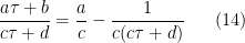
We will give some examples of modular functions (beyond the trivial example of constant functions) shortly, but let us first observe that when one differentiates a modular function one gets a more general class of function, known as a modular form. In more detail, observe from (14) that the derivative of the Möbius transformation ${\tau \mapsto \frac{a\tau+b}{c\tau+d}}$ is ${\frac{1}{(c\tau+d)^2}}$ , and hence by the chain rule and (15) the derivative of a modular function ${f}$ would obey the variant law

$\displaystyle f'(\frac{a\tau+b}{c\tau+d}) = (c\tau+d)^2 f'(\tau).$

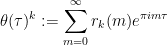
Motivated by this, we can define a (weakly) modular form of weight ${k}$ for any natural number ${k}$ to be a meromorphic function ${f: {\bf H} \rightarrow {\bf C} \cup \{\infty\}}$ which obeys the modularity relation

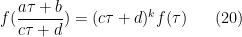$\displaystyle f(\frac{a\tau+b}{c\tau+d}) = (c\tau+d)^k f(\tau) \ \ \ \ \ (20)$

for all ${\tau \in {\bf H}}$ and all integers ${a,b,c,d}$ with ${ad-bc=1}$ (with the convention that ${c \infty = \infty}$ for any non-zero complex ${c}$ ), and which is meromorphic at the cusp ${\infty}$ in the sense of (16). Thus for instance modular functions are weakly modular forms of weight ${0}$ . A modular form of weight ${k}$ is a weakly modular form ${f}$ of weight ${k}$ which is holomorphic (not just meromorphic) on ${{\bf H}}$ , and also “holomorphic at ${\infty}$ ” in the sense that ${f(\tau)}$ is bounded for ${\mathrm{Im}(\tau)}$ large enough. Note that as viewed a function ${f(\tau) = \tilde f(e^{2\pi i \tau}) = \tilde f(q)}$ of the nome ${q = e^{2\pi i \tau}}$ , a modular form ${f}$ can be thought of as a certain type of holomorphic function ${\tilde f}$ on the disk ${D(0,1)}$ (using the Riemann singularity removal theorem to remove the singularity at the origin ${q=0}$ ), while weakly modular forms (and in particular modular functions) are certain types of meromorphic functions on this disk. A modular form that vanishes at infinity is known as a cusp form.

Exercise 23 Let ${k}$ be a natural number. Show that a function ${f: {\bf H} \rightarrow {\bf C}}$ obeys (20) if and only if it is ${1}$ -periodic in the sense of (18) and obeys the law
$\displaystyle f(-1/\tau) = \tau^k f(\tau) \ \ \ \ \ (21)$
for all ${\tau \in {\bf H}}$ .

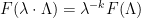
Exercise 24 (Lattice interpretation of modular forms) Let ${f}$ be a modular form of weight ${k}$ . Show that there is a unique function ${F}$ from lattices ${\Lambda}$ to complex numbers such that
$\displaystyle f(\tau) = F({\bf Z} + \tau {\bf Z})$
for all ${\tau \in {\bf H}}$ , and such that one has the homogeneity relation
$\displaystyle F(\lambda \cdot \Lambda) = \lambda^{-k} F(\Lambda)$
for any lattice ${\Lambda}$ and non-zero complex number ${\lambda}$ .

Observe that the product of a modular form of weight ${k}$ and a modular form of weight ${l}$ is a modular form of weight ${k+l}$ , and that the ratio of two modular forms of weight ${k}$ will be a modular function (if the denominator is not identically zero). Also, the space of modular forms of a given weight is a vector space, as is the space of modular functions. This suggests a way to generate non-trivial modular functions, by first locating some modular forms and then taking suitable rational combinations of these forms.

Somewhat analogously to how we used Lemma 3 to investigate the spaces ${L(D)}$ for divisors ${D}$ on a torus, we will investigate the space of modular forms via the following basic formula:

Theorem 25 (Valence formula) Let ${f}$ be a modular form of weight ${k}$ , not identically zero. Then we have
$\displaystyle \sum_\rho \mathrm{ord}_\rho(f) + \frac{1}{2} \mathrm{ord}_i(f) + \frac{1}{3} \mathrm{ord}_{e^{\pi i}/3}(f) + \mathrm{ord}_\infty(f) = \frac{k}{12} \ \ \ \ \ (22)$
where ${\mathrm{ord}_\rho}$ is the order of vanishing of ${f}$ at ${\rho}$ , ${\mathrm{ord}_\infty(f)}$ is the order of vanishing of ${\tilde f(q) := f(\tau)}$ (i.e., ${f}$ viewed as a function of the nome ${q = e^{2\pi i \tau}}$ ) at ${q=0}$ , and ${\rho}$ ranges over the zeroes of ${f}$ that are not equivalent to ${i, e^{\pi i/3}, \infty}$ , with just one zero counted per equivalence class. (This will be a finite sum.)

Informally, this formula asserts that the point ${i}$ only “deserves” to be counted in ${X_0(1)}$ with multiplicity ${1/2}$ due to its order ${2}$ stabiliser, while the point ${e^{\pi/3}}$ only “deserves” to be counted in ${X_0(1)}$ with multiplicity ${1/3}$ due to its order ${3}$ stabiliser. (The cusp ${\infty}$ has an infinite stabiliser, but this is compensated for by taking the order with respect to the nome variable ${q}$ rather than the period ratio variable ${\tau}$ .) The general philosophy of weighting points by the reciprocal of the order of their stabiliser occurs throughout mathematics; see this blog post for more discussion.

Proof: Firstly, from Exercise 22, we can place all the zeroes ${\rho}$ in the fundamental domain ${{\mathcal F}}$ . When parameterised in terms of the nome ${q}$ , this domain is compact, hence has only finitely many zeros, so the sum in (22) is finite.

As in the proof of Lemma 3(ii), we use the residue theorem. For simplicity, let us first suppose that there are no zeroes on the boundary of the fundamental domain ${{\mathcal F}}$ except possibly at the cusp ${\infty}$ . Then for ${T}$ large enough, we have from the residue theorem that

$\displaystyle \sum_\rho \mathrm{ord}_\rho(f) = \frac{1}{2\pi i} \int_\gamma \frac{f'(z)}{f(z)}\ dz,$

where ${\gamma}$ is the closed contour consisting of the polygonal path ${\gamma_{\frac{1}{2}+\frac{\sqrt{3}i}{2} \rightarrow \frac{1}{2} + iT \rightarrow -\frac{1}{2}+iT \rightarrow -\frac{1}{2}+\frac{\sqrt{3}i}{2}}}$ concatenated with the circular arc ${\{ e^{i(2\pi/3 - \theta)}: 0 \leq \theta \leq \pi/3 \}}$ . From the ${1}$ -periodicity, the contribution of the two vertical edges ${\gamma_{\frac{1}{2}+\frac{\sqrt{3}i}{2} \rightarrow \frac{1}{2} + iT}}$ and ${\gamma_{-\frac{1}{2}+iT \rightarrow -\frac{1}{2}+\frac{\sqrt{3}i}{2}}}$ cancel each other out. The contribution of the horizontal edge ${\gamma_{\frac{1}{2}+iT \rightarrow -\frac{1}{2}+iT}}$ can be written using the change of variables ${q = e^{2\pi i \tau}}$ as

$\displaystyle -\frac{1}{2\pi i} \int_{\gamma_{0,e^{-2\pi T},\circlearrowleft}} \frac{\tilde f'(q)}{\tilde f(q)}\ dq$

which by the residue theorem is equal to ${-\mathrm{ord}_\infty(f)}$ . Finally, using the modularity (21), one calculates that the contribution of the left arc ${\{ e^{i(2\pi/3 - \theta)}: 0 \leq \theta \leq \pi/6 \}}$ is equal to ${k/12}$ minus the contribution of the right arc ${\{ e^{i(2\pi/3 - \theta)}: \pi/6 \leq \theta \leq \pi/3 \}}$ . This gives the proof of the valence theorem in the case that there are no zeroes on the boundary of ${{\mathcal F}}$ .

Suppose now that there is a zero on the right edge ${\frac{1}{2}+it}$ of ${{\mathcal F}}$ , and hence also on the left edge ${-\frac{1}{2}+it}$ by periodicity, for some ${t > \frac{\sqrt{3}}{2}}$ . One can account for this zero by perturbing the contour ${\gamma}$ to make a little detour to the right of ${\frac{1}{2}+it}$ (e.g., by a circular arc), and a matching detour to the right of ${-\frac{1}{2}+it}$ . One can then verify that the same argument as before continues to work, with this boundary zero being counted exactly once. Similarly, if there is a zero on the left arc ${e^{i\theta}}$ for some ${\pi/2 < \theta < 2\pi/3}$ , and hence also at ${e^{i(\pi-\theta)}}$ by modularity, one can make a detour slightly above ${e^{i\theta}}$ and slightly below ${e^{i(\pi-\theta)}}$ (with the two detours being related by the transform ${\tau \mapsto -1/\tau}$ to ensure cancellation), and again we can argue as before. If instead there is a zero at ${i}$ , one makes an (approximately) semicircular detour above ${i}$ ; in this case the detour does not cancel out, but instead contributes a factor of ${\frac{1}{2} \mathrm{ord}_i(f)}$ in the limit as the radius of the detour goes to zero. Finally, if there is a zero at ${e^{i\pi/3}}$ (and hence also at ${e^{2\pi i/3}}$ ), one makes detours by two arcs of angle approximately ${\pi/3}$ at these two points; these two (approximate) sixth-circles end up contributing a factor of ${\frac{1}{2} \mathrm{ord}_{e^{\pi i/3}}(f)}$ in the limit, giving the claim. $\Box$

Exercise 26 (Quick applications of the valence formula)

(i) Let ${f}$ be a modular form of weight ${k}$ , not identically zero. Show that ${k}$ is equal to ${0}$ or an even number that is at least ${4}$ .
(ii) (Liouville theorem for ${X_0(1)}$ ) If ${f}$ is a modular form of weight zero, show that it is constant. (Hint: apply the valence theorem to various shifts ${f-c}$ of ${f}$ by constant.)
(iii) For ${k=4,6,8,10,14}$ , show that the vector space of modular forms of weight ${k}$ is at most one dimensional. (Hint: in these cases, there are a very limited number of solutions to the equation ${a + \frac{1}{2} b + \frac{1}{3} c = \frac{k}{12}}$ with ${a,b,c}$ natural numbers.)
(iv) Show that there are no cusp forms of weight ${k}$ when ${k < 12}$ or ${k=14}$ , and for ${k=12}$ the space of cusp forms of weight ${k}$ is at most one dimensional.
(v) Show that for any ${k}$ , the space of cusp forms of weight ${k}$ is a subspace of the space of modular forms of weight ${k}$ of codimension at most one, and that both spaces are finite-dimensional.

A basic example of modular forms are provided by the Eisenstein series

$\displaystyle G_k( \Lambda ) := \sum_{z \in \Lambda \backslash \{0\}} \frac{1}{z^{k}} \ \ \ \ \ (23)$

that we have already encountered for even integers ${k = 4,6,8,\dots}$ greater than two (we ignore the odd Eisenstein series as they vanish). We can view this as a function on ${{\bf H}}$ by the formula

$\displaystyle G_k( \tau) := G_k( {\bf Z} + \tau {\bf Z} ). \ \ \ \ \ (24)$

Observe that if ${a,b,c,d}$ are integers with ${ad-bc = 1}$ , then

$\displaystyle {\bf Z} + \frac{a\tau+b}{c\tau+d} {\bf Z} = \frac{1}{c\tau+d} ( (c\tau+d) {\bf Z} + (a\tau+b) {\bf Z} ) = \frac{1}{(c\tau+d)} ({\bf Z} + \tau {\bf Z})$

using the matrix inverse in ${SL_2({\bf Z})}$ . Inserting this into (23), (24) we conclude that

$\displaystyle G_k( \frac{a\tau+b}{c\tau+d} ) = (c\tau+d)^k G_k(\tau).$

(Compare also with Exercise 24.) Also, from (23), (24) we have

$\displaystyle G_k(\tau) = \sum_{(n,m) \in {\bf Z}^2 \backslash \{(0,0)\}} \frac{1}{(n+m\tau)^{k}}. \ \ \ \ \ (25)$

The series here is locally uniformly convergent for ${\tau \in {\bf H}}$ , so ${G_k}$ is holomorphic. Also, using the bounds

$\displaystyle \sum_{n \in {\bf Z}} \frac{1}{|n+m\tau|^k} \lesssim \sum_{n \in {\bf Z}} \min( \frac{1}{|n + m \mathrm{Re} \tau|^k}, \frac{1}{|m \mathrm{Im} \tau|^k} )$

$\displaystyle \lesssim \int_{\bf R} \min( \frac{1}{t^k}, \frac{1}{|m \mathrm{Im} \tau|^k} )\ dt$

$\displaystyle \lesssim \frac{1}{|m \mathrm{Im} \tau|^{k-1}}$

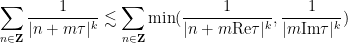
for non-zero ${m}$ , while

$\displaystyle \sum_{n \in {\bf Z} \backslash 0} \frac{1}{n^k} = 2 \zeta(k) \ \ \ \ \ (26)$

where ${\zeta(k)}$ is the famous Riemann zeta function

$\displaystyle \zeta(k) := \sum_{n=1}^\infty \frac{1}{n^k},$

we conclude on summing in ${m}$ and using the hypothesis ${k>2}$ that

$\displaystyle G_k(\tau) = 2 \zeta(k) + O_k( \frac{1}{|\mathrm{Im}(\tau)|^{k-1}}).$

In particular, ${G_k}$ is bounded at infinity. Summarising, we have established that the Eisenstein series ${G_k}$ is a modular form of weight ${k}$ , which is not identically zero (since it approaches the non-zero value ${2 \zeta(k)}$ at the cusp ${\infty}$ ). Combining this with Exercise 26(iii), we see that we have completely classified the modular forms of weight ${k}$ for ${k=4,6,8,10,14}$ , namely they are the scalar multiples of ${G_k}$ . For instance, the coefficients

$\displaystyle g_2(\tau) = 60 G_4(\tau)$

and

$\displaystyle g_3(\tau) = 140 G_6(\tau)$

appearing in the previous section are modular forms of weight ${4}$ and weight ${6}$ respectively, and the modular discriminant

$\displaystyle \Delta(\tau) = g_2^3(\tau) - 27 g_3^2(\tau)$

from Exercise 10 is a modular form of weight ${12}$ . From that exercise, this modular form never vanishes on ${{\bf H}}$ , hence by the valence formula it must have a simple zero at ${\infty}$ , and in particular is a cusp form. From Exercise 26 it is the unique cusp form of weight ${12}$ , up to constants.

Exercise 27 Give an alternate proof that ${\Delta}$ is a cusp form, not using the valence identity, by first establishing that ${\zeta(4) = \frac{\pi^4}{90}}$ and ${\zeta(6) = \frac{\pi^6}{945}}$ .

We can now create our first non-trivial modular function, the ${j}$ -invariant

$\displaystyle j(\tau) := 1728 \frac{g_2(\tau)^3}{\Delta(\tau)}.$

The factor of ${1728}$ is traditional, as it gives a nice normalisation at ${\infty}$ , as we shall see later. One can take advantage of complex multiplication to compute two special values immediately:

Lemma 28 We have ${j(i) = 1728}$ and ${j(e^{\pi i/3})=0}$ .

Proof: Using the rotation symmetry ${z \mapsto iz}$ we see that ${G_6(i) = 0}$ , hence ${g_3(i)=0}$ which implies that ${\Delta(i)=g_2(i)^3}$ and hence ${j(i)=1728}$ . Similarly, using the rotation symmetry ${z \mapsto e^{\pi i/3} z}$ we have ${G_4(e^{\pi i/3}) = 0}$ , hence ${j(e^{\pi i/3}=0)}$ . (One can also use the valence formulae to get the vanishing ${G_6(i)=G_4(e^{\pi i/3})=0}$ ). $\Box$

Being modular, we can think of ${j}$ as a map from ${X_0(1)}$ to ${{\bf C}}$ . We have the following fundamental fact:

Proposition 29 The map ${j: X_0(1) \rightarrow {\bf C}}$ is a bijection.

Proof: Note that for any ${\lambda \in {\bf C}}$ , ${j(\tau) = 1728 \lambda}$ if and only if ${\tau}$ is a zero of ${g_2^3 - \lambda \Delta}$ . It thus suffices to show that for every ${\lambda \in {\bf C}}$ , the zeroes of the function ${g_2^3 - \lambda \Delta}$ in ${{\bf H}}$ consist of precisely one orbit of ${SL_2({\bf Z})}$ . This function is a modular form of weight ${12}$ that does not vanish at infinity (since ${g_2}$ does not vanish while ${\Delta}$ does). By the valence formula, we thus have

$\displaystyle \sum_\rho \mathrm{ord}_\rho( g_2^3 - \lambda \Delta ) + \frac{1}{2} \mathrm{ord}_1( g_2^3 - \lambda \Delta ) + \frac{1}{3} \mathrm{ord}_{e^{\pi i/3}}( g_2^3 - \lambda \Delta ) = 1.$

As the orders are all natural numbers, some case checking reveals that there are now only three possibilities:

${g_2^3 - \lambda \Delta}$ has a simple zero at precisely one ${SL_2({\bf Z})}$ -orbit, not equivalent to ${1}$ or ${e^{\pi i/3}}$ .
${g_2^3 - \lambda \Delta}$ has a double zero at ${i}$ (and equivalent points), and no other zeroes.
${g_2^3 - \lambda \Delta}$ has a triple zero at ${e^{\pi i/3}}$ (and equivalent points), and no other zeroes.

In any of these three cases, the claim follows. $\Box$

Note that this proof also shows that ${j(\tau)-1728}$ has a double zero at ${i}$ and ${j(\tau)}$ has a triple zero at ${e^{\pi i/3}}$ , but that ${j(\tau)-j(\tau_0)}$ has a simple zero for any ${\tau_0 \in {\bf H}}$ not equivalent to ${i}$ or ${e^{\pi i/3}}$ .

We can now give the entire modular curve ${X_0(1)}$ the structure of a Riemann surface by declaring ${j}$ to be the coordinate function. This is compatible with the existing Riemann surface structure on ${X_0(1)'}$ since ${j}$ was already holomorphic on this portion of the curve. Any modular function ${f}$ can then factor as ${f(\tau) = F(j(\tau))}$ for some meromorphic function ${F}$ that is initially defined on the punctured complex plane ${{\bf C} \backslash \{ 0, 1728 \}}$ ; but from meromorphicity of ${f}$ on ${{\bf H}}$ and at infinity we see that ${F}$ blows up at an at most polynomial rate as one approaches ${0}$ , ${1728}$ , or ${\infty}$ , and so ${F}$ is in fact a meromorphic function on the entire Riemann sphere and is thus a rational function (Exercise 19 of 246A Notes 4). We conclude

Proposition 30 Every modular function is a rational function of the ${j}$ -invariant ${j}$ .

Conversely, it is clear that every rational function of ${j}$ is modular, thus giving a satisfactory description of the modular functions.

Exercise 31 Show that every modular function is the ratio of two modular forms of equal weight (with the denominator not identically zero).

Exercise 32 (All elliptic curves are tori) Let ${A, B}$ be two complex numbers with ${A^3 - 27B^3 \neq 0}$ . Show that there is a lattice ${\Lambda}$ such that ${g_2(\Lambda) = A}$ and ${g_3(\Lambda) = B}$ , so in particular the elliptic curve
$\displaystyle \{ (z,w): w^2 = 4 z^3 - A z - B \} \cup \{\infty\}$
is complex diffeomorphic to a torus ${\Lambda \backslash {\bf C}}$ .

Remark 33 By applying some elementary algebraic geometry transformations one can show that any (smooth, irreducible) cubic plane curve ${\{ (z,w): P(z,w) = 0 \}}$ generated by a polynomial ${P: {\bf C} \times {\bf C} \rightarrow {\bf C}}$ of degree ${3}$ is a Riemann surface complex diffeomorphic to a torus ${\Lambda \backslash {\bf C}}$ after adding some finite number of points at infinity; also, some degree ${4}$ curves such as
$\displaystyle \{ (z,w): w^2 = (z-a)(z-b)(z-c)(z-d) \} \cup \{\infty\}$
can also be placed in this form. However we will not detail the required transformations here.

A famous application of the theory of the ${j}$ -invariant is to give a short Riemann surface-based proof of the the little Picard theorem (first proven in Theorem 55 of 246A Notes 4):

Theorem 34 (Little Picard theorem) Let ${f: {\bf C} \rightarrow {\bf C}}$ be entire and non-constant. Then ${f({\bf C})}$ omits at most one point of ${{\bf C}}$ .

Proof: Suppose for contradiction that ${f({\bf C})}$ omits at least two points of ${{\bf C}}$ . By applying a linear transformation, we may assume that ${f}$ omits the points ${0}$ and ${1728}$ . Then ${j^{-1} \circ f}$ is a holomorphic function from ${{\bf C}}$ to ${X_0(1)' = PSL_2({\bf Z}) \backslash {\bf H}'}$ . Since the domain ${{\bf C}}$ is simply connected, ${j^{-1} \circ f}$ lifts to a holomorphic function from ${{\bf C}}$ to ${{\bf H}}$ . Since ${{\bf H}}$ is complex diffeomorphic to a disk, this lift must be constant by Liouville’s theorem, hence ${f}$ is constant as required. (This is essentially Picard’s original proof of this theorem.) $\Box$

The great Picard theorem can also be proven by a more sophisticated version of these methods, but it requires some study of the possible behavior of elements of ${SL_2({\bf Z})}$ ; see Exercise 37 below.

All modular forms are ${1}$ -periodic, and hence by Proposition 1 should have a Fourier expansion, which is also a Laurent expansion in the nome. As it turns out, the Fourier coefficients often have a highly number-theoretic interpretation. This can be illustrated with the Eisenstein series ${G_k}$ ; here we follow the treatment in Stein-Shakarchi. To compute the Fourier coefficients we first need a computation:

Exercise 35 Let ${k \geq 2}$ and ${\tau \in {\bf H}}$ , and let ${q := e^{2\pi i \tau}}$ be the nome. Establish the identity
$\displaystyle \sum_{n \in {\bf Z}} \frac{1}{(n+\tau)^k} = \frac{(-2\pi i)^k}{(k-1)!} \sum_{\ell=1}^\infty \ell^{k-1} q^\ell$
in two different ways:

(i) By applying the Poisson summation formula (Proposition 3(v) of Notes 2).
(ii) By first establishing the identity
$\displaystyle \sum_{n \in {\bf Z}} \frac{1}{(n+\tau)^2} = \frac{\pi^2}{\sin^2(\pi \tau)} \ \ \ \ \ (27)$
by applying Proposition 1 to the difference of the two sides, and differentiating in ${\tau}$ . (You may also establish (27) by other means, such as differentiating and then manipulating the identities in Exercises 25 or 27 of Notes 1.)

From (25), (26) (and symmetry) one has

$\displaystyle G_k(\tau) = 2 \zeta(k) + 2 \sum_{m=1}^\infty \sum_{n \in {\bf Z}} \frac{1}{(n+m\tau)^k}$

and hence by the above exercise

$\displaystyle G_k(\tau) = 2 \zeta(k) + 2 \frac{(-2\pi i)^k}{(k-1)!} \sum_{m=1}^\infty \sum_{\ell=1}^\infty \ell^{k-1} q^{m\ell}.$

Since ${|q|<1}$ it is not difficult to show that the double sum here is absolutey convergent and can be rearranged as we please. If we group the terms based on the product ${r=m\ell}$ we thus have the Fourier expansion

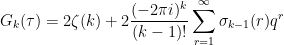
$\displaystyle G_k(\tau) = 2 \zeta(k) + 2 \frac{(-2\pi i)^k}{(k-1)!} \sum_{r=1}^\infty \sigma_{k-1}(r) q^r$

where the ${(k-1)^{th}}$ divisor function ${\sigma_{k-1}(r)}$ is defined by

$\displaystyle \sigma_{k-1}(r) := \sum_{\ell|r} \ell^{k-1}$

where the sum is over those natural numbers ${\ell}$ that divide ${r}$ . Thus for instance

$\displaystyle G_4(\tau) = 2 \zeta(4) + \frac{2(2\pi)^4}{3!} \sum_{r=1}^\infty \sigma_3(r) q^r$

$\displaystyle = \frac{\pi^4}{45} ( 1 + 240 \sum_{r=1}^\infty \sigma_3(r) q^r )$

$\displaystyle = \frac{\pi^4}{45} ( 1 + 240 q + \dots )$

and

$\displaystyle G_6(\tau) = 2 \zeta(6) - \frac{2(2\pi)^6}{5!} \sum_{r=1}^\infty \sigma_5(r) q^r$

$\displaystyle = \frac{2\pi^6}{945} ( 1 - 504 \sum_{r=1}^\infty \sigma_5(r) q^r )$

$\displaystyle = \frac{2\pi^6}{945} ( 1 - 504 q - \dots )$

so after some calculation

$\displaystyle g_2(\tau) = \frac{4 \pi^4}{3} (1 + 240 q + \dots )$

$\displaystyle g_3(\tau) = \frac{8 \pi^6}{27} (1 - 504 q - \dots)$

$\displaystyle \Delta(\tau) = (2\pi)^{12} (q - \dots)$

and therefore

$\displaystyle j(\tau) = q^{-1} + \dots, \ \ \ \ \ (28)$

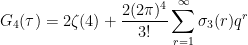
thus the factor of ${1728}$ in the definition of the ${j}$ -invariant normalises the “residue” of ${j}$ at infinity to equal ${1}$ .

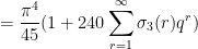
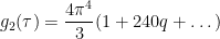
Remark 36 If one expands out a few more terms in the above expansions, one can calculate
$\displaystyle j(z) = q^{-1} + 744 + 196884 q + 21493760 q^2 + \dots. \ \ \ \ \ (29)$
The various coefficients in here have several remarkable algebraic properties. For instance, applying this expansion at ${\tau = (1 + \sqrt{-d})/2}$ for a natural number ${d}$ , so that ${q = -e^{-\pi \sqrt{d}}}$ , one obtains the approximation
$\displaystyle j( (1 + \sqrt{-d})/2 ) = - e^{\pi \sqrt{d}} + 744 + O( e^{-\pi \sqrt{d}} ).$
Now for certain values of ${d}$ , most famously ${d = 163}$ , the torus ${({\bf Z} + (1 + \sqrt{-d})/2 {\bf Z}) \backslash {\bf C}}$ admits a complex multiplication that allows for computation of the ${j}$ -invariant by algebraic means (think of this as a more advanced version of Lemma 28; it is closely related to the fact that the ring of algebraic integers in ${{\bf Q}(\sqrt{-163})}$ admit unique factorisation, see these previous notes for some related discussion). For instance, one can eventually establish that
$\displaystyle j( (1 + \sqrt{-163})/2 ) = (-640320)^3$
which eventually leads to the famous approximation
$\displaystyle e^{\pi \sqrt{163}} \approx 640320^3 + 744$
(first observed by Hermite, but also attributed to Ramanujan via an April Fools’ joke of Martin Gardner) which is accurate to twelve decimal places. The remaining coefficients have a remarkable interpretation as dimensions of components of a certain representation of the monster group known as the moonshine module, a phenomenon known as monstrous moonshine. For instance, the smallest irreducible representation of the monster group has dimension ${196883}$ , precisely one less than the ${q}$ coefficient of ${j}$ . 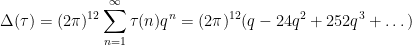The Fourier coefficients ${\tau(n)}$ of the (normalised) modular discriminant,
$\displaystyle \Delta(\tau) = (2\pi)^{12} \sum_{n=1}^\infty \tau(n) q^n = (2\pi)^{12} (q - 24 q^2 + 252 q^3 + \dots)$
form a sequence known as the Ramanujan ${\tau}$ function and obeys many remarkable properties. For instance, there is the totally non-obvious fact that this function is multiplicative in the sense that ${\tau(nm) = \tau(n) \tau(m)}$ whenever ${n,m}$ are coprime; see Exercise 43.

Exercise 37 (Great Picard theorem)

(i) Show that every fractional linear transformation ${\gamma: z \mapsto \frac{az+b}{cz+d}}$ on ${{\bf H}}$ with ${a,b,c,d \in {\bf Z}}$ , ${ad-bc=1}$ is either of finite order (elliptic case), conjugate to a translation ${z \mapsto z+h}$ for some ${h > 0}$ after conjugating by another fractional linear transformation (parabolic case), or conjugate to a dilation ${z \mapsto \lambda z}$ for some ${\lambda >1}$ after conjugating by another fractional linear transformation (hyperbolic case). (Hint: study the eigenvalues and eigenvectors of ${\begin{pmatrix} a & b \\ c& d\end{pmatrix}}$ , based on the value of the trace ${a+d}$ and in particular whether the magnitude of the trace is less than two, equal to two, or greater than two. Note that the trace also has to be an integer.)
(ii) Let ${f: D(0,1) \backslash \{0\} \rightarrow {\bf C} \backslash \{0,1728\}}$ be holomorphic. Show that there exists a holomorphic function ${F: {\bf H} \rightarrow {\bf H}}$ such that ${j(F(z)) = f(e^{2\pi i z})}$ for all ${z \in {\bf H}}$ , as well as a fractional linear transformation ${\gamma:\frac{az+b}{cz+d}}$ with ${a,b,c,d \in {\bf Z}}$ and ${ad-bc=1}$ such that ${F(z+1) = \gamma(F(z))}$ for all ${z \in {\bf H}}$ .
(iii) If the transformation ${\gamma}$ in (ii) is in the elliptic case of (i), show that ${f}$ is bounded in a neighbourhood of ${0}$ , and hence has a removable singularity at the origin. (Hint: ${F}$ will have some finite period and can thus be studied using Proposition 1 after applying a Möbius transform to map ${{\bf H}}$ to a disk.)
(iv) If the transformation ${\gamma}$ in (ii) is in the hyperbolic case of (i), show that ${f}$ is bounded in a neighbourhood of ${0}$ , and hence has a removable singularity at the origin. (Hint: The standard branch of ${z \mapsto z^{2\pi i / \log\lambda}}$ maps ${{\bf H}}$ to an annulus, and is invariant with respect to the dilation action ${z \mapsto \lambda z}$ . Use this to create a bounded ${1}$ -periodic holomorphic function on ${{\bf H}}$ .)
(v) If the transformation ${\gamma}$ in (ii) is in the parabolic case of (i), show that ${f}$ exhibits at most polynomial growth as one approaches ${0}$ , and hence has at most a pole at the origin. (Hint: If for instance ${F(z+1)=F(z)+h}$ , then ${F(z)-h z}$ is ${1}$ -periodic and takes values in ${{\bf H}}$ , and one can now repeat the arguments of (iii). Also use the expansion (28).)
(vi) Use the previous parts of this exercise to give another proof of the great Picard theorem (Theorem 56 of 245A Notes 4): the image of a holomorphic function in a punctured disk ${D(z_0,r) \backslash \{z_0\}}$ with an essential singularity at ${z_0}$ omits at most one value of ${{\bf C}}$ .

Exercise 38 (Dimension of space of modular forms)

(i) If ${k}$ is an even natural number, show that the dimension of the space of modular forms of weight ${k}$ is equal to ${\lfloor k/12\rfloor+1}$ except when ${k}$ is equal to ${2}$ mod ${12}$ , in which case it is equal to ${\lfloor k/12\rfloor}$ . (Hint: for ${k \leq 12}$ this follows from Exercise 26; to cover the larger ranges of ${k}$ , use the modular discriminant ${\Delta}$ to show that the space of cusp forms of weight ${k+12}$ is isomorphic to the space of modular forms of weight ${k}$ .
(ii) If ${k}$ is an even natural number, show that a basis for the space of modular forms of weight ${k}$ is provided by the powers ${G_4^i G_6^j}$ where ${i,j}$ range over natural numbers (including zero) with ${4i+6j=k}$ .

Thus far we have constructed modular forms and modular functions starting from Eisenstein series ${G_k}$ . There is another important, and seemingly quite different, way to generate modular forms coming from theta functions. Typically these functions are not quite modular in the sense given in these notes, but are close enough that after some manipulation one can transform theta functions into modular forms. The simplest example of a theta function is the Jacobi theta function

$\displaystyle \theta(\tau) := \sum_{n \in {\bf Z}} e^{\pi i n^2 \tau}, \ \ \ \ \ (30)$

which is easily seen to be a holomorphic function on ${{\bf H}}$ that goes to zero as ${\mathrm{Im}(\tau) \rightarrow +\infty}$ . It is not quite a modular form, but is ${2}$ -periodic (instead of ${1}$ -periodic) in the sense that

$\displaystyle \theta(\tau+2) = \theta(\tau)$

for all ${\tau \in {\bf H}}$ , and from Poisson summation (see Exercise 7 of Notes 2) we have the variant

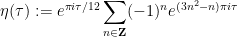
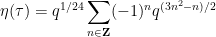
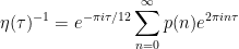
$\displaystyle \theta(-1/\tau) = (-i\tau)^{1/2} \theta(\tau)$

of the modularity relation (21), using the standard branch of the square root. This is not quite modular in nature, but a slight variant of the theta function fares better:

Exercise 39 Define the Dedekind eta function ${\eta: {\bf H} \rightarrow {\bf C}}$ by the formula
$\displaystyle \eta(\tau) := e^{\pi i \tau/12} \sum_{n \in {\bf Z}} (-1)^n e^{(3n^2-n) \pi i \tau}$
or in terms of the nome ${q = e^{2\pi i \tau}}$
$\displaystyle \eta(\tau) = q^{1/24} \sum_{n \in {\bf Z}} (-1)^n q^{(3n^2-n)/2}$
where ${q^{1/24}}$ is one of the ${24^{th}}$ roots of ${q}$ .

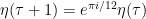
(i) Establish the modified ${1}$ -periodicity
$\displaystyle \eta(\tau+1) = e^{\pi i/12} \eta(\tau)$
and the modified modularity
$\displaystyle \eta(-1/\tau) = (-i\tau)^{1/2} \eta(\tau)$
using the standard branch of the square root. (Hint: a direct application of Poisson summation applied to ${\eta(-1/\tau)}$ gives a sum that looks somewhat like ${\eta(\tau)}$ but with different numerical constants (in particular, one sees terms like ${e^{\pi i n^2 \tau/3}}$ instead of ${e^{3\pi i n^2 \tau}}$ arising). 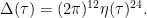Split the index of summation ${n}$ into three components ${n = 3m}$ , ${n=3m+1}$ , ${n=3m+2}$ based on the residue classes modulo ${3}$ and rearrange each component separately.)
(ii) Establish the identity
$\displaystyle \Delta(\tau) = (2\pi)^{12} \eta(\tau)^{24}.$
(Hint: show that both sides are cusp forms of weight ${12}$ that vanish like ${(2\pi)^{12} q}$ near the cusp.)

Remark 40 The relationship between ${\Delta}$ and the ${24^{th}}$ power of the eta function can be interpreted (after some additional effort) as a relation ${\Theta_\Lambda = G_{12} - \frac{65520}{691} \Delta}$ between the modular discriminant ${\Delta}$ and the theta function ${\Theta_\Lambda(\tau) := \sum_{x \in \Lambda} e^{-i\pi \tau \|x\|^2}}$ of a certain highly symmetric ${24}$ -dimensional lattice ${\Lambda \subset {\bf R}^{24}}$ known as the Leech lattice, but we will not pursue this connection further here.

The ${\eta}$ function has a remarkable factorisation coming from Euler’s pentagonal number theorem

$\displaystyle \sum_{n \in {\bf Z}} (-1)^n q^{(3n^2-n)/2} = \prod_{m=1}^\infty (1 - q^m), \ \ \ \ \ (31)$

so that

$\displaystyle \eta(\tau) = e^{\pi i \tau/12} \prod_{m=1}^\infty (1 - e^{2\pi i m \tau}). \ \ \ \ \ (32)$

There are many proofs of the pentagonal number theorem in the literature. One approach is to first establish the more general Jacobi triple product identity:

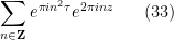
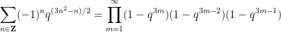
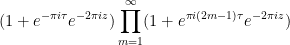
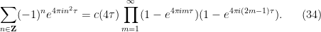
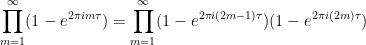
Theorem 41 (Jacobi triple product identity) For any ${\tau \in {\bf H}}$ and ${z \in{\bf C}}$ , one has
$\displaystyle \sum_{n \in {\bf Z}} e^{\pi i n^2 \tau} e^{2\pi i nz} \ \ \ \ \ (33)$

$\displaystyle = \prod_{m=1}^\infty (1 - e^{2\pi i m \tau}) (1 + e^{\pi i (2m-1) \tau} e^{2\pi i z}) (1 + e^{\pi i (2m-1) \tau} e^{-2\pi i z}).$

Observe that by replacing ${\tau}$ by ${3\tau/2}$ and ${z}$ with ${1/2 - \tau/4}$ we have

$\displaystyle \sum_{n \in {\bf Z}} (-1)^n q^{(3n^2-n)/2} = \prod_{m=1}^\infty (1 - q^{3m}) (1 - q^{3m-2}) (1-q^{3m-1})$

and this gives the identity (31) after splitting the integers into the three residue classes ${3m, 3m-2, 3m-1}$ modulo ${3}$ . One can obtain many further identities of this type by other substitutions; for instance, by setting ${z=0}$ in the triple product identity, one obtains

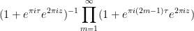
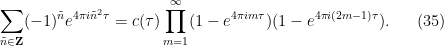
$\displaystyle \theta(\tau) = \prod_{n=1}^\infty (1 - e^{2\pi i nz}) (1 + e^{\pi i (2n-1)z})^2.$

Proof: Let us denote the left-hand side and right-hand side of (33) by ${\Theta(z|\tau)}$ and ${\Pi(z|\tau)}$ respectively. For fixed ${\tau \in {\bf H}}$ , both sides are clearly holomorphic in ${z}$ , with ${\Pi(z|\tau)}$ . Our strategy in showing that ${\Theta}$ and ${\Pi}$ agree (following Stein-Shakarchi) is to first observe that they have many of the same periodicity properties. We clearly have ${1}$ -periodicity

$\displaystyle \Theta(z+1|\tau) = \Theta(z|\tau); \quad \Pi(z+1|\tau) = \Pi(z|\tau).$

From the identity

$\displaystyle e^{\pi i n^2 \tau} e^{2\pi i n(z+\tau)} = e^{-\pi i \tau} e^{-2\pi i z} e^{\pi i (n+1)^2 \tau} e^{2\pi i (n+1)z}$

we also have the modified ${\tau}$ -periodicity

$\displaystyle \Theta(z+\tau|\tau) = e^{-\pi i \tau} e^{-2\pi i z} \Theta(z|\tau);$

similarly from the telescoping products

$\displaystyle \prod_{m=1}^\infty (1 + e^{\pi i (2m-1) \tau} e^{2\pi i (z+\tau)}) = \prod_{m=1}^\infty (1 + e^{\pi i (2(m+1)-1) \tau} e^{2\pi i z})$

$\displaystyle (1 + e^{\pi i \tau} e^{2\pi i z})^{-1} \prod_{m=1}^\infty (1 + e^{\pi i (2m-1) \tau} e^{2\pi i z})$

and

$\displaystyle \prod_{m=1}^\infty (1 + e^{\pi i (2m-1) \tau} e^{-2\pi i (z+\tau)}) = \prod_{m=1}^\infty (1 + e^{\pi i (2(m-1)-1) \tau} e^{-2\pi i z})$

$\displaystyle (1 + e^{-\pi i \tau} e^{-2\pi i z}) \prod_{m=1}^\infty (1 + e^{\pi i (2m-1) \tau} e^{-2\pi i z})$

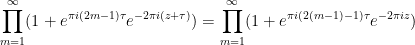
we conclude that ${\Pi}$ also obeys the same modified ${\tau}$ -periodicity

$\displaystyle \Pi(z+\tau|\tau) = e^{-\pi i \tau} e^{-2\pi i z} \Pi(z|\tau).$

Thus the ratio ${z \mapsto \Theta(z|\tau)/\Pi(z|\tau)}$ is meromorphic and doubly periodic. Furthermore, one checks that ${\Pi(z|\tau)}$ only vanishes when ${z}$ is equal to ${\frac{1+\tau}{2}}$ modulo ${{\bf Z} + \tau{\bf Z}}$ with a simple zero at those locations, so the ratio ${z \mapsto \Theta(z|\tau)/\Pi(z|\tau)}$ has at most a single simple pole on the torus ${{\bf Z} + \tau {\bf Z} \backslash {\bf C}}$ and thus constant by the discussion after Lemma 6 (alternatively, one can show that ${\Theta(z|\tau)}$ also vanishes at this point and apply Proposition 2). Thus there is some quantity ${c(\tau)}$ depending only on ${\tau}$ for which we have the identity

$\displaystyle \Theta(z|\tau) = c(\tau) \Pi(z|\tau)$

for all ${z \in {\bf H}}$ . To exploit this, we first set ${z = 1/2}$ and replace ${\tau}$ by ${4\tau}$ to conclude that

$\displaystyle \sum_{n \in {\bf Z}} (-1)^n e^{4\pi i n^2 \tau} = c(4\tau) \prod_{m=1}^\infty (1 - e^{8\pi i m \tau}) (1 - e^{4\pi i (2m-1) \tau})^2$

but on rearranging the absolutely convergent product we have

$\displaystyle \prod_{m=1}^\infty (1 - e^{8\pi i m \tau}) (1 - e^{4\pi i (2m-1) \tau}) = \prod_{m=1}^\infty (1 - e^{4\pi i m \tau})$

and thus

$\displaystyle \sum_{n \in {\bf Z}} (-1)^n e^{4\pi i n^2 \tau} = c(4\tau) \prod_{m=1}^\infty (1 - e^{4\pi i m \tau}) (1 - e^{4\pi i (2m-1) \tau}). \ \ \ \ \ (34)$

If instead we set ${z=1/4}$ and not modify ${\tau}$ , we have

$\displaystyle \sum_{n \in {\bf Z}} i^n e^{\pi i n^2 \tau} = c(\tau) \prod_{m=1}^\infty (1 - e^{2\pi i m \tau}) (1 + e^{2\pi i (2m-1) \tau});$

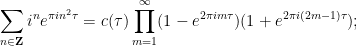the contribution of ${n}$ and ${-n}$ on the left-hand sides cancel when ${n}$ is odd, so that on making the substitution ${n = 2\tilde n}$ we obtain

$\displaystyle \sum_{n \in {\bf Z}} i^n e^{\pi i n^2 \tau} = \sum_{\tilde n \in {\bf Z}} (-1)^{\tilde n} e^{4\pi i \tilde n^2 \tau}$

while from rearranging an absolutely convergent product we have

$\displaystyle \prod_{m=1}^\infty (1 - e^{2\pi i m \tau}) = \prod_{m=1}^\infty (1 - e^{2\pi i (2m-1) \tau}) (1 - e^{2\pi i (2m) \tau})$

and thus by difference of two squares

$\displaystyle \sum_{\tilde n \in {\bf Z}} (-1)^{\tilde n} e^{4\pi i \tilde n^2 \tau} = c(\tau) \prod_{m=1}^\infty (1 - e^{4\pi i m \tau}) (1 - e^{4\pi i (2m-1) \tau}). \ \ \ \ \ (35)$

Comparing this with (34) we obtain the surprising additional symmetry

$\displaystyle c(\tau) = c(4\tau). \ \ \ \ \ (36)$

On the other hand, taking limits in (say) (35) we see that ${c(\tau) \rightarrow 1}$ as ${\mathrm{Im} \tau \rightarrow +\infty}$ . If we then iterate (36) we conclude that

$\displaystyle c(\tau) = \lim_{j \rightarrow \infty} c(4^j \tau) = 1$

and the claim follows. $\Box$

Remark 42 Another equivalent form of (32) is
$\displaystyle \eta(\tau)^{-1} = e^{-\pi i \tau/12} \sum_{n=0}^\infty p(n) e^{2\pi i n \tau}$
where ${p(n)}$ is the partition function of ${n}$ – the number of ways to represent ${n}$ as the sum of positive integers (up to rearrangement). Among other things, this formula can be used to ascertain the asymptotic growth of ${p(n)}$ (which turns out to roughly be of the order of ${\exp( \pi \sqrt{2n/3} )}$ , as famously established by Hardy and Ramanujan).

Theta functions can be used to encode various number-theoretic quantities involving quadratic forms, such as sums of squares. For instance, from (30) and collecting terms one obtains the formula

$\displaystyle \theta(\tau)^k := \sum_{m=0}^\infty r_k(m) e^{\pi i m \tau}$

for any natural number ${k}$ , where ${r_k(m)}$ denotes the number of ways to express a natural number ${m}$ as the sum ${m = n_1^2 + \dots + n_k^2}$ of ${k}$ squares of integers. From Fourier inversion (Proposition 1 and a rescaling) one then has a representation

$\displaystyle r_k(m) = \frac{1}{2} \int_{\gamma_{\tau_0 \rightarrow \tau_0+2}} \theta(\tau)^k e^{-\pi i m \tau}\ d\tau$

for any ${\tau_0 \in {\bf H}}$ , which allows one to obtain asymptotics for ${r_k}$ when ${k}$ is large through estimation of the theta function (this is an example of the circle method); moreover, explicit identities relating the theta function to other near-modular forms (such as the Eisenstein series and their relatives) can be used to obtain exact formulae for ${r_k(m)}$ for small values of ${k}$ that can be used for instance to establish the famous Lagrange four-square theorem that all natural numbers are the sum of four squares. We refer the reader to the Stein-Shakarchi text for an exposition of this connection.

Exercise 43 (Hecke operators) Let ${k}$ be a natural number.

(i) If ${f}$ is a modular form of weight ${k}$ , and ${F}$ is the corresponding function on lattices given by Exercise 24, and ${m}$ is a positive natural number, show that there is a unique modular form ${T_m f}$ of weight ${k}$ whose corresponding function ${G}$ on lattices is related to ${F}$ by the formula
$\displaystyle G(\Lambda) := m^{k-1} \sum_{\Lambda' \subset \Lambda: [\Lambda:\Lambda'] = m} F(\Lambda')$
where the sum ranges over all sublattices ${\Lambda'}$ of ${\Lambda}$ whose index ${[\Lambda:\Lambda']}$ is equal to ${m}$ . Show that ${T_m}$ is a linear operator on the space of weight ${k}$ modular forms that also maps the space of weight ${k}$ cusp forms to itself; this operator is known as a Hecke operator.
(ii) Give the more explicit formula
$\displaystyle T_m f(\tau) = m^{k-1} \sum_{a,d>0: ad=m} \frac{1}{d^k} \sum_{b=0}^{d-1} f( \frac{az+b}{d} ).$

(iii) Show that the Hecke operators all commute with each other, thus ${T_n T_m f = T_m T_n f}$ whenever ${f}$ is a modular form of weight ${k}$ and ${n,m}$ are positive natural numbers. Furthermore show that ${T_n T_m = T_{nm}}$ if ${n,m}$ are coprime.
(iv) If ${f}$ is a modular form of weight ${k}$ with Fourier expansion ${f(\tau) = \sum_{n=0}^\infty a_n q^n}$ , show that for any coprime positive integers ${n,m}$ that the ${q^n}$ coefficient of ${T_m f}$ is equal to ${a_{nm}}$ .
(v) Establish the multiplicativity ${\tau(nm) = \tau(n) \tau(m)}$ of the Ramanujan tau function (the Fourier coefficients of the modular discriminant). (Hint: use the one-dimensionality of the space of cusp forms of weight ${12}$ to conclude that ${\Delta}$ is a simultaneous eigenfunction of the Hecke operators.)
Simultaneous eigenfunctions of the Hecke operators are known as Hecke eigenfunctions and are of major importance in number theory.

55 comments

Comments feed for this article

2 February, 2021 at 9:18 pm

On the notes on applications

Would number theoretic and sphere packing applications be covered in the class and would the notes be posted?

[No, I am not planning to cover those topics in this course. -T]

3 February, 2021 at 2:12 am

Anonymous

The top-level tags of this post appear to have the wrong course tagging.

[Fixed, thanks – T.]

3 February, 2021 at 2:47 am

Anonymous

typo in Lemma 6: P should be in the torus, not in \Lambda

[Corrected, thanks – T.]

3 February, 2021 at 2:51 am

Anonymous

Lemma 3 is referred to as Lemma 2.

[Corrected – T]

3 February, 2021 at 6:58 am

Anonymous

I think there’s a typo in the first paragraph: \omega Z\C should be C/\omega Z

[Both forms are acceptable. In the case of quotients of actions by abelian groups it makes little difference, but when it comes to nonabelian groups such as ${\bf SL}_2({\bf Z})$ the convention matters a little bit, and I have elected to have the groups act on the left and define quotients accordingly. -T]

3 February, 2021 at 12:59 pm

Anonymous

The product representation of $\eta$ function is closely related to the product representation of the generating function for the partition function $p(n)$ (and can be used to derive its convergent asymptotic series)

[A remark to this effect has been added, thanks – T.]

4 February, 2021 at 12:13 pm

Anonymous

The identity (8) can also be proved by observing (via Laurent expansion coefficients) that its LHS is entire – so by proposition 2 it is a constant.

4 February, 2021 at 12:22 pm

Anonymous

Correction: I meant that the difference(!) between the LHS and the RHS (not the LHS) of (8) is entire – so it must be a constant.

[An exercise to this effect has been added – T.]

4 February, 2021 at 5:15 pm

Lior Silberman

For a different approach to Exercise 17, note that if $\gamma\in\mathrm{SL}_2(\mathbb{Z})$ fixes a point in $\mathbb{H}$ then it lies in the intersection of a discrete group and a compact group, hence had finite order.

Its eigenvalues must then be roots of unity which are also quadratic irrationalities. Since a primitive root of unity of order $n$ has degree $\phi(n)$ , we see that the order must be one of 1,2,3,4,6. This computes the cojugacy classes of these elements.

Also, dividing by $\pm I$ which act trivially we see that $\gamma$ has order 1,2,3 in $\mathrm{PSL}_2(\mathbb{Z})$ .

5 February, 2021 at 9:31 am

Terence Tao

Thanks for this! One can also see that an element of $SL_2({\bf Z})$ that has roots of unity as eigenvalues must have trace in the set $\{-2, -1, 0, 1, 2\}$ which also gives the eigenvalues and thus the conjugacy class in ${\bf SL}_2({\bf R})$ . But I was not able to easily show that any two such elements of $SL_2({\bf Z})$ with the same eigenvalues were conjugate in $SL_2({\bf Z})$ (which is what one needs to specify the fixed points) without messing around with lattices as in the stated exercise. (Maybe this is just some consequence of the algebraic integer nature of the eigenvalues, but I didn’t immediately see an argument.)

11 February, 2021 at 6:24 am

Jarek Kuben

This argument can be finished using the shape of the standard fundamental domain. With notation as above, if $\gamma\cdot\tau=\tau$ for $\gamma\ne\pm I$ , then $c\ne0$ and we can WLOG assume $c>0$ by replacing $\gamma$ with $-\gamma$ if necessary. This equation also implies that $(\tau,1)^T$ is an eigenvector of $\gamma$ with eigenvalue $c\tau+d$ , and since $c\tau+d\in\bf H$ , it’s $c\tau+d\in\{i,(\pm1+i\sqrt3)/2\}$ . But if we also WLOG assume $\tau\in\mathcal F$ , then it follows that $\tau\in\{i,(\pm1+i\sqrt3)/2\}$ .

12 February, 2021 at 3:53 pm

Lior Silberman

Let $\gamma\in\Gamma = \mathrm{SL}_2(\mathbb{Z})$ be an element of finite order (other than $\pm I$ ) with characteristic polynomial $p(x)=x^2-tx+1 \in \mathbb{Z}[x]$ where $t=\mathbb{Tr}\gamma$ , and consider $\mathbb{Z}^2$ as a module of over the commutative subring $\mathbb{Z}[\gamma] \subset M_2(\mathbb{Z})$ .

As a ring we have $\mathbb{Z}[\gamma] \equiv \mathbb{Z}[x]/(p) \equiv \mathbb{Z}[\zeta]$ where $\zeta$ is a root of $p$ , that is a primitive root of unity of order 3,4,6. It so happens that $\mathcal{O}=\mathbb{Z}[\zeta]$ is the ring of integers of the quadratic field $\mathbb{Q}(\zeta)$ , and that these rings of integers are PIDs (in fact both these rings are Euclidean). By the classification of modules over a PID and since $\mathbb{Z}^2$ is torsion-free we see that $\mathbb{Z}^2$ is isomorphic to $\mathcal{O}$ as an $\mathcal{O}$ -module.

Now if $\gamma,\delta$ are two such elements then we get an isomorphism $\eta\colon\mathbb{Z}^2\to\mathbb{Z}^2$ intertwining the two $\mathcal{O}$ -module structures, in other words an element of $\mathrm{GL}_2(\mathbb{Z})$ conjugating $\gamma,\delta$ .

12 February, 2021 at 6:35 pm

Terence Tao

Nice! So a little bit of algebraic number theory allows one to show the transitivity of the $SL_2({\bf Z})$ action amongst all elements of finite order with fixed characteristic polynomial. (Unfortunately this argument is difficult to work into this complex analysis class as it requires a set of prerequisites that are basically disjoint from those already assumed for this course.)

12 February, 2021 at 7:07 pm

Lior Silberman

By the way you can also apply the same idea to the hyperbolic elements (those with $|t|>2$ ). The the ring $\mathbb{Z}[\gamma]$ is an order in the corresponding real quadratic field $\mathbb{Q}(\sqrt{t^2-4})$ (a subring which is also a lattice), it is not hard to show $\mathbb{Z}^2$ is one of the ideal classes of the order. We thus obtain the well-known bijection between closed geodesics on the modular surface and ideal classes in quadratic orders.

12 February, 2021 at 7:08 pm

Lior Silberman

(and I forgot to add to the bijection the conjugacy classes in the modular group of [primitive] hyperbolic elements)

3 June, 2023 at 12:07 pm

Jarek Kuben

It’s also possible to combine the lattice and algebraic number theory approaches in a way that perhaps gives more insight and shows that the two exceptional orbits are related to complex multiplication.

Indeed, let $\tau\in\mathbf H$ be a fixed point of $\gamma=\begin{pmatrix}a&b\\c&d\end{pmatrix}\in\mathrm{SL}_2(\mathbf Z)$ , then $[\tau,1]=[a\tau+b,c\tau+d]=(c\tau+d)[\frac{a\tau+b}{c\tau+d},1]$ , thus $c\tau+d\in\mathrm{Aut}(\Lambda)$ , where $\Lambda=[\tau,1]$ . We claim that the map $\mathrm{Stab}(\tau)\to\mathrm{Aut}(\Lambda)\le\mathbf C^\times$ given by $\gamma\to c\tau+d$ is a group isomorphism. Indeed, it’s easy to check that it’s a homomorphism, and it’s injective since $c\tau+d=1$ implies $c=0$ , $d=1$ , and then $a=1$ , and thus $\tau=\gamma\cdot\tau=\tau+b$ , and so $b=0$ and $\gamma=I$ . It’s also surjective since for $\lambda\in\mathrm{Aut}(\Lambda)$ the couple $(\lambda\tau,\lambda)$ is a $\mathbf Z$ -basis of $\Lambda$ with $\mathrm{Im}(\lambda\tau/\lambda)=\mathrm{Im}(\tau)>0$ , and so there exists $\gamma\in\mathrm{SL}_2(\mathbf Z)$ such that $\lambda\begin{pmatrix}\tau\\1\end{pmatrix}=\gamma\begin{pmatrix}\tau\\1\end{pmatrix}$ , which implies $\gamma\in\mathrm{Stab}(\tau)$ and $\gamma\to\lambda$ .

However for a lattice $\Lambda$ it’s $\mathrm{End}(\Lambda)=\mathbf Z$ and thus $\mathrm{Aut}(\Lambda)=\mathbf Z^\times=\pm1$ , except for the case when $\Lambda$ is a scalar multiple of an invertible ideal in some imaginary quadratic order $\mathcal O$ , in which case it’s $\mathrm{End}(\Lambda)=\mathcal O$ and $\mathrm{Aut}(\Lambda)=\mathcal O^\times$ .

It follows that $\tau$ has a stabilizer larger that $\pm I$ iff $\Lambda=[\tau,1]$ is a scalar multiple of an invertible ideal in an imaginary quadratic order that has units other that $\pm1$ . However the only such orders are $\mathbf Z[i]$ and $\mathbf Z[\zeta_3]$ , and they both have trivial class group, thus $\Lambda$ is a scalar multiple of $\mathbf Z[i]$ or $\mathbf Z[\zeta_3]$ , and so $\tau$ belongs to the orbit of $i$ or $\zeta_3$ .

Furthermore it’s $\mathrm{Stab}(i)\cong\mathrm{Aut}(\mathbf Z[i])=\mathbf Z[i]^\times=\langle i\rangle\cong\mathbf Z/4$ and $\mathrm{Stab}(\zeta_3)\cong\mathrm{Aut}(\mathbf Z[\zeta_3])=\mathbf Z[\zeta_3]^\times=\langle\zeta_6\rangle\cong\mathbf Z/6$ , and we can use the above map to explicitly compute these stabilizers. Indeed, it’s $i\begin{pmatrix}i\\1\end{pmatrix}=\begin{pmatrix}0&-1\\1&0\end{pmatrix}\begin{pmatrix}i\\1\end{pmatrix}$ and $\zeta_6\begin{pmatrix}\zeta_3\\1\end{pmatrix}=\begin{pmatrix}0&-1\\1&1\end{pmatrix}\begin{pmatrix}\zeta_3\\1\end{pmatrix}$ , hence $\mathrm{Stab}(i)=\left\langle\begin{pmatrix}0&-1\\1&0\end{pmatrix}\right\rangle$ and $\mathrm{Stab}(\zeta_3)=\left\langle\begin{pmatrix}0&-1\\1&1\end{pmatrix}\right\rangle$ .

5 February, 2021 at 5:43 am

Anonymous

Professor Tao, in the proof of Great Picard’s theorem, why is it that $j^{-1}\circ f(e^{iz})$ lifts to a 1-periodic function?

[Oops, this is an issue. It can be resolved by analysing the possible shifts by elements of ${SL}_2({\bf Z})$ that can occur, but this is a little tricky. For now I have deleted the proof of the theorem, will think more about whether there is a painless fix to it. UPDATE: now an exercise. -T]

5 February, 2021 at 11:01 am

Anonymous

In exercise 34 it seems that $\int$ should be $\sum$

[Corrected, thanks – T.]

5 February, 2021 at 12:56 pm

Anonymous

In the proof of theorem 39, it seems that there are some latex problems in some formulas.

[Fixed now – T.]

6 February, 2021 at 10:04 am

Anonymous

In remark 42 it seems (from the product representation of the generating function for $p(n)$ ) that the summand $p(0) := 1$ should also be included in the displayed sum.

[Corrected, thanks – T.]

7 February, 2021 at 10:14 am

Anonymous

In the first line of proposition 1, it seems that “periodic” should appear between “singly” and “holomorphic”.

[Corrected, thanks – T.]

9 February, 2021 at 4:01 am

Anonymous

In proposition 2, the periods should be linearly independent over $\mathbb R$ (not $\mathbb C$ )

[Corrected, thanks – T.]

9 February, 2021 at 4:19 am

Anonymous

In exercise 37, the statement of the great Picard theorem is missing.

[Added, thanks – T.]

13 February, 2021 at 2:10 pm

Anonymous

I don’t know if this is the best place to put it, but there is a typo remark 40 (descriminant)

16 February, 2021 at 7:41 am

Anonymous

Should Lemma 6 be codimension at most 1, i.e. 0 or 1?

[Corrected, thanks – T.]

16 February, 2021 at 8:11 pm

RJD

I admit, I’m a little puzzled in exercise 43. I am reading Serre’s “A course in Arithmetic” and looking at the Hecke operator section. He defines T_m(f) in the way I expect (i.e., using the notation above, T_m(f)(z)=G(z,1)). However, he derives that this is a modular form using the more explicit expression in part (ii). Is there some way of concluding that this is the unique modular form with lattice function G without using the expression directly?

18 February, 2021 at 3:42 pm

Terence Tao

Yes; $G$ is clearly a function on $\Lambda$ (so different generators give rise to the same value of $G$ ) and obeys the same homogeneity relation as $F$ does (see Exercise 24), so modularity can be proven rather painlessly without needing the explicit expansion in (ii).

19 February, 2021 at 6:00 pm

RJD

Okay, so I have a dumb question. I agree that weak modularity follows fairly easily. What about holomorphicity at infinity? What am I missing here? It seems Serre does what he does to establish the holomorphicity at infinity, so I was wondering specifically about how that is taken care of.

22 February, 2021 at 6:18 pm

Terence Tao

There are only a bounded number of sublattices $\Lambda'$ of $\Lambda$ of a fixed index (note that all lattices are isomorphic to each other as abelian groups, so once one has finiteness for say ${\bf Z}^2$ one has finiteness for the rest), so if $F$ is bounded at infinity then so is $G$ . (Holomorphicity can be established by a similar argument.) Part (ii) comes from actually enumerating these bounded number of sublattices, but this isn’t necessary for the qualitative properties in (i).

24 February, 2021 at 11:44 pm

RJD

Thank you so much for your responses Professor Tao! One more question. You mention that F being bounded at infinity implies that G is bounded at infinity, and that holomorphicity can be established by a similar argument. What do you mean by bounded at infinity? Do you mean that the associated modular function given by Exercise 24 is bounded as $Im(\tau) \rightarrow \infty$?

[Yes – T.]

27 February, 2021 at 9:14 am

Course announcement: 246B, complex analysis | What's new

[…] Elliptic functions and their relatives; […]

27 February, 2021 at 9:37 am

246B, Notes 2: Some connections with the Fourier transform | What's new

[…] Previous set of notes: Notes 1. Next set of notes: Notes 3. […]

27 February, 2021 at 9:40 am

246B, Notes 4: The Riemann zeta function and the prime number theorem | What's new

[…] set of notes: Notes 3. Next set of notes: 246C Notes […]

12 February, 2022 at 12:13 pm

Throughout the notes, you have used both ${\bf R}/{\bf Z}$ (as in the “additive unit circle”) and something like $\Lambda\backslash {\bf C}$ . Are there any reasons for the preferences?

14 February, 2022 at 8:45 am

Terence Tao

For abelian actions the two notations are interchangeable. For non-abelian actions like $\mathrm{SL}_2({\mathbf{Z}}) \backslash \mathbf{H}$ one has to use the left quotient if one wants the group $SL_2({\bf Z})$ to act on the left, so I set up my notation for Riemann surface structures on quotient spaces using left quotients (and I have tried to emphasise the analogy between the torus $\Lambda \backslash {\bf C}$ and the modular curve $\mathrm{SL}_2({\mathbf{Z}}) \backslash \mathbf{H}$ in these notes). But I am not viewing the unit circle ${\bf R}/{\bf Z}$ as part of a larger class of possibly non-abelian quotient spaces, so here I am happy to use the traditional right quotient notation.

13 April, 2022 at 2:50 pm

If one has a group $X$ and $X$ being a normal subgroup of $X$ , then one has the quotient group $X/G$ .

In this set of notes, it seems to be the case that $X$ is just a set and $G$ being any group acting on $X$ ; and you talk about the “quotient” $G/X$ or $X\backslash G$ . Is there a group structure hiding somewhere for the set $X$ ? Also, is there a “normal subgroup” lurking somewhere?

19 April, 2022 at 8:54 am

Terence Tao

One can quotient out any set by any equivalence relation to obtain a quotient space. In particular, any group acting on a space gives rise to a quotient space through the orbit equivalence relation. For instance, one can quotient any group $G$ by any subgroup $H$ to obtain a quotient space $G/H$ (of left-cosets) or $H \backslash G$ (of right cosets). The normality of $H$ is only required if one wants this quotient space to also be a group.

16 April, 2022 at 3:22 pm

In the proof of Lemma 3(iii), the path ${\gamma_{0 \rightarrow \omega_j}}$ is not closed. What modification of the argument principle is used?

19 April, 2022 at 9:18 am

Terence Tao

While the path $\gamma_{0 \to \omega_j}$ is not closed, the image $f \circ \gamma_{0 \to \gamma_j}$ is. Apply a change of variables $w = f(z)$ to conclude.

16 April, 2022 at 4:19 pm

Consider the example of $f(z)=z-1$ and $D=0(P)$ where $P=1$ . According to the notes, $L(D)=L(0)$ consists of only constant functions and thus $f\not\in L(D)$ by the definition.

But I got $(f)=1(P)$ because the order of zero is $1$ at $P$ . So $(f)+D\ge 0$ and thus $f\in L(D)$ .

16 April, 2022 at 4:20 pm

What is going wrong in the calculation above?

[The function $f(z)=z-1$ is not elliptic (doubly periodic) and so does not give a well-defined holomorphic function on the torus. -T.]

17 April, 2022 at 6:37 am

… To figure out which, we can normalise ${P}$ to be the origin coset ${\Lambda}$ . The question is now whether there is a doubly periodic meromorphic function that has a double pole at each point of ${\Lambda}$ . A naive candidate for such a function would be the infinite series
$\displaystyle \sum_{z_0 \in \Lambda} \frac{1}{(z-z_0)^2},$
however this series turns out to not be absolutely convergent.

I am confused with the reasoning here.

The goal was to study the dimension of $L(2\cdot(P))$ , which is at least $1$ since every constant function ${f: \Lambda \backslash {\bf C} \rightarrow {\bf C} \cup \{\infty\}}$ (or equivalently, a doubly periodic function ${f: {\bf C} \rightarrow {\bf C} \cup \{\infty\}}$ ) satisfies $(f)+2\cdot(P)\geq 0$ . So question is now whether

– there is a meromorphic function ${f: \Lambda \backslash {\bf C} \rightarrow {\bf C} \cup \{\infty\}}$ that has a double pole at $P=\Lambda$ ;

– or equivalently, a doubly periodic (meromorphic) function ${f: {\bf C} \rightarrow {\bf C} \cup \{\infty\}}$ that has a double pole at some point of $\Lambda$ .

(Why should it be that “The question is now whether there is a doubly periodic meromorphic function that has a double pole at each point of ${\Lambda}$ .”? Isn’t it that any single point in $\Lambda$ is a representative of the coset?)

What is really the equivalent way to say “poles” for meromorphic function ${f: \Lambda \backslash {\bf C} \rightarrow {\bf C} \cup \{\infty\}}$ and meromorphic function ${f: {\bf C} \rightarrow {\bf C} \cup \{\infty\}}$ ?

19 April, 2022 at 9:22 am

Terence Tao

If a doubly periodic function $f: {\bf C} \to {\bf C} \cup \infty$ has a pole at any point $z$ , it will also have a pole (of the same order) at every other point in the coset $z+\Lambda$ by periodicity, and so when viewed as a function $f: \Lambda \backslash {\bf C} \to {\bf C} \cup \infty$ , it can be said to have a pole at the point $z+\Lambda \in \Lambda \backslash {\bf C}$ (of the specified order).

17 April, 2022 at 9:26 am

Minor typo in (6):

$\displaystyle \wp(z) := \frac{1}{z^2} + \sum_{z_0 \in \Lambda \backslash 0} \frac{1}{(z-z_0)^2} - \frac{1}{z_0^2} \ \ \ \ \ (6)$

is meant to be

$\displaystyle \wp(z) := \frac{1}{z^2} + \sum_{z_0 \in \Lambda \backslash \{0\}} \left(\frac{1}{(z-z_0)^2} - \frac{1}{z_0^2}\right) \ \ \ \ \ (6)$

[Corrected, thanks – T.]

17 April, 2022 at 12:08 pm

In proving the double periodicity of the function $\wp$ , it is said that

… The series on the right is absolutely convergent, and on every coset of ${\omega_1 {\bf Z}}$ it telescopes to zero.

Cosets of $\Lambda\backslash{\bf C}$ is of the form $\lambda+\Lambda$ for some $\lambda\in{\bf C}$ . What do you mean by “coset of ${\omega_1 {\bf Z}}$ “?

[A set of the form $z + \omega_1 {\bf Z}$ for some complex number $z$ . -T.]

18 April, 2022 at 4:46 pm

In (11): $\wp(z')$ –> $\wp'(z)$ .

… we have ${1/z = h^{-1}(w/z^2)}$ in a neighbourhood of infinity.

–>

… we have ${1/z = h^{-1}((w/z^2)^2)}$ in a neighbourhood of infinity.

[Corrected, thanks – T.]

20 April, 2022 at 12:56 pm

… so to demonstrate absolute convergence it suffices to show that
$\displaystyle \sum_{z_0 \in \Lambda: z_0 \neq 0} \frac{1}{|z_0|^3} < \infty.$
But a simple volume packing argument (considering the areas of the translates ${z_0 + D}$ of the fundamental domain ${D}$ ) shows that the number of lattice points ${z_0}$ in any disk ${D(0,R)}$ , ${R \geq 1}$ is ${O_\Lambda(R^2)}$ , and so by dyadic decomposition as in Notes 1, the series is absolutely convergent.

Can you please elaborate on what the “volume packing argument” is?

22 April, 2022 at 8:56 am

Terence Tao

As $z_0$ ranges over the lattice points in the disk $D(0,R)$ , the translates $z_0+D$ of the fundamental domain each have area $|D|$ and are disjoint (up to null sets) and occupy (a subset of) a disk of radius $R + O(1)$ , which has area $O(R^2)$ . So the total number of such lattice points is at most $O(R^2) / |D| = O_\Lambda(R^2)$ .
(The same argument also gives a comparable lower bound.)

20 April, 2022 at 1:55 pm

If ${a}$ lies in the half-lattice ${\frac{1}{2} \Lambda}$ but not in ${\Lambda}$ (thus, it lies in one of the half-periods ${\frac{\omega_1}{2} + \Lambda}$ , ${\frac{\omega_2}{2} + \Lambda}$ , or ${\frac{\omega_1+\omega_2}{2} + \Lambda}$ ) then from the even and doubly periodic nature of ${\wp}$ we see that ${\wp(a+z) = \wp(a-z)}$ for all ${z \not \in \frac{1}{2} \Lambda}$ , so ${\wp - \wp(a)}$ in fact must have at least a double zero at ${a}$ ,…

If $a$ lies in one of the half-periods, isn’t it true for *all* $z$ that
$\wp(a+z)=\wp(-a-z)=\wp(a-z)$ ? (I guess the notes just want to emphasize that it is particularly true for $z\not\in\frac{1}{2}\Lambda$ . Correct?) How does this fact imply that $\wp-\wp(a)$ must have at least a double zero at $a$ ?

20 April, 2022 at 2:19 pm

Also, why is it not possible that when $a$ is a half-period, $\wp-\wp(a)$ has a simple zero at $a$ , and another simple zero at another half-period?

22 April, 2022 at 8:58 am

Terence Tao

The exclusion $z \not \in \frac{1}{2} \Lambda$ is solely to avoid the poles of $\wp$ . Applying the even symmetry $\wp(a+z) = \wp(a-z)$ to the Taylor expansion of $\wp$ around $a$ , we see that only the even power coefficients can be non-zero, hence the order of any zero of $\wp - \wp(a)$ at $a$ must be even.

21 April, 2022 at 11:27 am

Are there relations between “elliptic curves” and “modular curves” in this set of notes? It seems that according to the definition in Section 2, a modular curve is a set of equivalent classes of elliptic curves. Is there anything more than that?

22 April, 2022 at 9:06 am

Terence Tao

There are additional, much deeper, connections between elliptic curves and modular forms, most notably through the modularity theorem that asserts that the L-function of an elliptic curve defined over the rationals has coefficients that are also the Fourier coefficients of a modular form (which, among other things, famously implies Fermat’s last theorem, and also serves as a special case for the broader Langlands program), but this is well beyond the scope of this course.

22 April, 2022 at 12:05 pm

… so that the function ${\wp(z) - \frac{1}{z^2}}$ , which extends holomorphically to the origin, has ${k^{th}}$ derivative at the origin equal to ${(-1)^k (k+1)! G_{k+2}(\Lambda)}$ ,

Without taking into account the fact that $G_k=0$ for odd $k$ , by direct calculation, should the derivative at the origin equal to

${ (k+1)! G_{k+2}(\Lambda)}$ instead?

Taking the $k$ -th derivative, one has

$(\wp(z)-\frac{1}{z^2})^{(k)}=(-1)^k(k+1)!\sum_{z_0\in\Lambda\setminus \{0\}}\frac{1}{(z-z_0)^{k+2}}$

Taking $z\to 0$ one has a factor of $(-1)^{k+2}$ in the denominator and thus cancel out with $(-1)^k$ .

[Updated, though by making the change of variables $z_0 \mapsto -z_0$ one could also have retained the $(-1)^k$ factor if desired. -T]

22 December, 2022 at 1:19 am

Anonymous

Where can I read more about the connection mentioned in Remark 40, between the Dedekind eta function and the theta function of the Leech lattice?

	Anonymous on Infinite partial sumsets in th…
	Anonymous on A Banach algebra proof of the…
	Anonymous on A Banach algebra proof of the…
	Aleksandar on 245C, Notes 4: Sobolev sp…
	Anonymous on Erratum for “An inverse…
	Anonymous on Erratum for “An inverse…
	Anonymous on Erratum for “An inverse…
	Anonymous on Erratum for “An inverse…
	Terence Tao on 245C, Notes 4: Sobolev sp…
	Terence Tao on 275A, Notes 3: The weak and st…
	Terence Tao on What is a gauge?
	Terence Tao on Erratum for “An inverse…
	Terence Tao on 275A, Notes 3: The weak and st…
	Terence Tao on An epsilon of room: pages from…
	Aleksandar on 245C, Notes 4: Sobolev sp…

246B, Notes 3: Elliptic functions and modular forms

Recent Comments

Articles by others

Diversions

Mathematics

Selected articles

Software

The sciences

Top Posts

Archives

Categories

The Polymath Blog

55 comments

Leave a comment Cancel reply

For commenters

246B, Notes 3: Elliptic functions and modular forms

Share this:

Recent Comments

Articles by others

Diversions

Mathematics

Selected articles

Software

The sciences

Top Posts

Archives

Categories

The Polymath Blog

55 comments

Leave a comment Cancel reply

For commenters