
Let X be a real-valued random variable, and let 
Weak law of large numbers. Suppose that the first moment
of X is finite. Then
converges in probability to
, thus
for every
.
Strong law of large numbers. Suppose that the first moment
.
[The concepts of convergence in probability and almost sure convergence in probability theory are specialisations of the concepts of convergence in measure and pointwise convergence almost everywhere in measure theory.]
(If one strengthens the first moment assumption to that of finiteness of the second moment 
The weak law is easy to prove, but the strong law (which of course implies the weak law, by Egoroff’s theorem) is more subtle, and in fact the proof of this law (assuming just finiteness of the first moment) usually only appears in advanced graduate texts. So I thought I would present a proof here of both laws, which proceeds by the standard techniques of the moment method and truncation. The emphasis in this exposition will be on motivation and methods rather than brevity and strength of results; there do exist proofs of the strong law in the literature that have been compressed down to the size of one page or less, but this is not my goal here.
— The moment method —
The moment method seeks to control the tail probabilities of a random variable (i.e. the probability that it fluctuates far from its mean) by means of moments, and in particular the zeroth, first or second moment. The reason that this method is so effective is because the first few moments can often be computed rather precisely. The first moment method usually employs Markov’s inequality
(which follows by taking expectations of the pointwise inequality 

(note that (2) is just (1) applied to the random variable 

Generally speaking, to compute the first moment one usually employs linearity of expectation

whereas to compute the second moment one also needs to understand covariances (which are particularly simple if one assumes pairwise independence), thanks to identities such as

or the normalised variant


Higher moments can in principle give more precise information, but often require stronger assumptions on the objects being studied, such as joint independence.
Here is a basic application of the first moment method:
Borel-Cantelli lemma. Let
be a sequence of events such that
is finite. Then almost surely, only finitely many of the events
are true.
Proof. Let 


Letting 

Returning to the law of large numbers, the first moment method gives the following tail bound:
Lemma 1. (First moment tail bound) If
is finite, then
.
Proof. By the triangle inequality, 

Lemma 1 is not strong enough by itself to prove the law of large numbers in either weak or strong form – in particular, it does not show any improvement as n gets large – but it will be useful to handle one of the error terms in those proofs.
We can get stronger bounds than Lemma 1 – in particular, bounds which improve with n – at the expense of stronger assumptions on X.
Lemma 2. (Second moment tail bound) If
.
Proof. A standard computation, exploiting (3) and the pairwise independence of the 


In the opposite direction, there is the zeroth moment method, more commonly known as the union bound

or equivalently (to explain the terminology “zeroth moment”)

for any non-negative random variables 
Just as the second moment bound (Lemma 2) is only useful when one has good control on the second moment (or variance) of X, the zeroth moment tail estimate (3) is only useful when we have good control on the zeroth moment 
— Truncation —
The second moment tail bound (Lemma 2) already gives the weak law of large numbers in the case when X has finite second moment (or equivalently, finite variance). In general, if all one knows about X is that it has finite first moment, then we cannot conclude that X has finite second moment. However, we can perform a truncation
of X at any desired threshold N, where 


and hence also we have finite variance

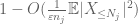
The second term 
By the triangle inequality, we conclude that the first term

These are all the tools we need to prove the weak law of large numbers:
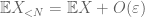
Proof of weak law. Let 


From (7), (8), we can find a threshold N (depending on 

From the first moment tail bound (Lemma 1), we know that 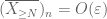


— The strong law —
The strong law can be proven by pushing the above methods a bit further, and using a few more tricks.
The first trick is to observe that to prove the strong law, it suffices to do so for non-negative random variables 

Once X is non-negative, we see that the empirical averages

Because of this quasimonotonicity, we can sparsify the set of n for which we need to prove the strong law. More precisely, it suffices to show
Strong law of large numbers, reduced version. Let
be a non-negative random variable with
, and let
be a sequence of integers which is lacunary in the sense that
for some
and all sufficiently large j. Then
converges almost surely to
Indeed, if we could prove the reduced version, then on applying that version to the lacunary sequence 


[This sparsification trick is philosophically related to the dyadic pigeonhole principle philosophy; see an old short story of myself on this latter topic. One could easily sparsify further, so that the lacunarity constant c is large instead of small, but this turns out not to help us too much in what follows.]
Now that we have sparsified the sequence, it becomes economical to apply the Borel-Cantelli lemma. Indeed, by many applications of that lemma we see that it suffices to show that

for non-negative X of finite first moment, any lacunary sequence 
[If we did not first sparsify the sequence, the Borel-Cantelli lemma would have been too expensive to apply; see Remark 2 below. Generally speaking, Borel-Cantelli is only worth applying when one expects the events
At this point we go back and apply the methods that already worked to give the weak law. Namely, to estimate each of the tail probabilities 

We should at least pick 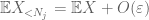


Now we look at the contribution of 

But there is one last card to play, which is the zeroth moment method tail estimate (4). As mentioned earlier, this bound is lousy in general – but is very good when X is mostly zero, which is precisely the situation with 


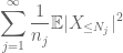
Putting this all together, we see that

Summing this in j, we see that we will be done as soon as we figure out how to choose
and
are both finite. (As usual, we have a tradeoff: making the
Based on the discussion earlier, it is natural to try setting 

and
(where the implied constant here depends on the sequence 
Remark 1. The above proof in fact shows that the strong law of large numbers holds even if one only assumes pairwise independence of the 

Remark 2. It is essential that the random variables 


Remark 3. From the perspective of interpolation theory, one can view the above argument as an interpolation argument, establishing an 


Remark 4. By viewing the sequence
[Update, Jul 19: some corrections.]
[Update, Jul 20: Connections with ergodic theory discussed.]

109 comments
Comments feed for this article
7 November, 2011 at 6:02 am
Note on the weak and strong laws of large numbers | Mathematics and me-themed antics.
[…] my development was different from that in the book. My notes essentially follow the proof given by Terry Tao, so you may want to refer to his notes as well. Like this:LikeBe the first to like this post. […]
21 January, 2012 at 3:00 pm
abc
It seems like the proof of the pointwise ergodic theorem is easier than this proof! Inspecting that proof, it uses the the added generality of measure-preserving systems to deal with functions that you could not talk about (naturally) in the setting of the strong law of large numbers.
4 February, 2013 at 9:05 pm
Iosif Pinelis
I think this result and proof are very nice. There is a vague commonality between Keane’s and Tao’s proof: both exploit, to an extent, the fact that the sample mean varies little, in a sense, with
  . It is also nice that Tao’s result is not contained in the ergodic theorem. Indeed, one can easily see that the pairwise independence does not imply the stationarity. E.g., let
  be defined as
  , respectively, where the
  ‘s are independent Rademacher random variables, each taking each of the values
  with probability 1/2. Define
  similarly, based on
  ; etc. Then the
  ‘s are pairwise independent. However,
  , whereas
  . So, the sequence
  is not stationary.
[LaTeX code corrected; the problem was the lack of a space between “latex” and the LaTeX code. Also, the curly braces were unnecessary. -T]
5 February, 2013 at 8:01 pm
Iosif Pinelis
Thank you for the help with LaTeX. A couple more points here:
(i) Of course, I wanted to say “the pairwise independence does not imply the stationarity, even if the ‘s are identically distributed”, rather than just “the pairwise independence does not imply the stationarity”.
(ii) Tao’s result, with the pairwise independence rather than with the complete independence, can be extended in a standard manner to the case when the ‘s take values in an arbitrary separable Banach space (say).
9 March, 2013 at 7:36 pm
Laws of large numbers and Birkhoff’s ergodic theorem | Vaughn Climenhaga's Math Blog
[…] including a different proof of the weak law than the one above, can be found on Terry Tao’s blog), we observe that the strong law of large numbers can be viewed as a special case of the Birkhoff […]
8 May, 2013 at 5:59 am
Mate Wierdl
Hi Terry! Maybe a few exercises could be added based on the following remarks:
If we assume finite second moment then only “multiplicativity” is needed. By multiplicativity, I mean . This translates to orthogonality if the expectations are $\latex 0$.
An application would be Weyl’s result: if is a sequence of integers then for almost all
  , the sequence
  is uniformly distributed
  . For this, we take
  .
.
With this mutiplicativity assumption, one can simply get results for random variables with varying expectations: Consider nonnegative random variables with varying expectation, but then we would divide by the expectation of the sum of the first $n$ random variables instead of to get the right normalization. For example, the expectations can go to
  arbitrary slowly as long as
  . But the expectations can also go to
  ! They cannot increase arbitrary fast: something like
  for
for  seems to be the limit for a strong law, while for norm (weak) convergence, one can get arbitrary close to
  , that is we can have
  .
.
I think these are good exercises for using and testing the limits of this "lacunary subsequence" trick.
4 October, 2013 at 4:46 pm
Paul
MISSING PARENTHESIS:
Ex1+,…+xn = E(x1) +…+E(xn)
should have the parenthesis on the left side of equation thus:
E(x1+…+xn) = E(x1)+…+E(xn)
5 February, 2014 at 7:46 am
Law of large numbers for dependent but uncorrelated random variables | Vaughn Climenhaga's Math Blog
[…] book “Probability and Measure”, where it is Theorem 22.1. There is also a discussion on Terry Tao’s blog, which emphasises the role of the main tools in this proof: the moment method and […]
10 February, 2014 at 9:30 am
Tomasz
Could someone provide some reference to a full proof of the “strong law for independent empirical means for the full sequence under second moment bounds” mentioned in Remark 2? Or at least could someone provide a more detailed explanation of the proof outlined in this remark, in particular what Chernoff’s inequality should be used and how?
28 May, 2014 at 6:38 am
Anonymous
Hi Dear Professor Tao.
I have a question. If you are an infinite number of random variables. You can still use the strong law of large numbers? please more explain for me.
best regards
5 June, 2015 at 8:49 pm
Prasenjit Karmakar
“Indeed, this follows immediately from the simple fact that any random variable X with finite first moment can be expressed as the difference of two non-negative random variables $\max(X,0), \max(-X,0)$ of finite first moment.”
To express a random variable as the difference of two, I think finite moment is not needed, it is needed when we express expectation as the difference of two.
Thanks.
1 July, 2015 at 11:06 am
Law of Large Numbers | Kepler lounge
[…] that the sample average converges in probability toward the expected value. There is also a Strong version which I won’t discuss further. But, both versions are of great importance in science as […]
4 December, 2015 at 12:08 pm
Possible explanation for a Bell experiment?
[…] be taken as an axiom? The Law Of Large Numbers: https://en.wikipedia.org/wiki/Law_of_large_numbers https://terrytao.wordpress.com/2008/06/18/the-strong-law-of-large-numbers/ QM explains what's going on in Bell. Why you want to come up with another I cant quite […]
9 February, 2016 at 4:03 am
Error : what is n in quantum mechanics | Physics Forums - The Fusion of Science and Community
[…] But as the number of systems in the ensemble tends to infinity the law of large numbers applies: https://terrytao.wordpress.com/2008/06/18/the-strong-law-of-large-numbers/ Don't worry about the proof if you don't know the math to follow it. Simply grasp what […]
22 July, 2016 at 8:24 am
Helmholtz: El Origen y Significado de los Axiomas Geométricos (1) | Divergiendo - «Nebar defiqueit mor danguot iuit»
[…] 13. Tao, T. (2008, 18th June). The strong law of large numbers. [Weblog]. Retrieved 17 July 2016, from https://terrytao.wordpress.com/2008/06/18/the-strong-law-of-large-numbers/#comment-41939↩ […]
6 October, 2016 at 8:10 pm
chaos
Hi prof Tao,
You wrote: “The concepts of convergence in probability and almost sure convergence in probability theory are specialisations of the concepts of convergence in measure and pointwise convergence almost everywhere in measure theory.”
In measure theory, is there any different between “pointwise convergence almost everywhere” and “convergence almost everywhere”?
[No – T.]
13 November, 2016 at 10:44 am
Anonymous
You might want to fix (3). The formula flows out.
[Corrected, thanks – T.]
19 March, 2017 at 10:36 pm
Nafisah
Nine years later, I’m finding this very helpful. Thank you
27 April, 2017 at 1:54 pm
ntthung
Dear Prof Tao,
One thing that’s been bothering me for a while: why is the absolute value sign used in the statement of the theorems? Why do we need E(|X|) instead of just E(X)?
Thank you.
28 April, 2017 at 9:12 am
Terence Tao
One cannot even define the expectation of a signed random variable unless one first knows that it is absolutely integrable (that is,
  ), since expectation is defined using Lebesgue integration.
28 April, 2017 at 2:07 pm
ntthung
Thank you very much. I was taught statistics in a slightly less formal way (without measure theory), but I guess it’s not too late to start.
28 April, 2017 at 5:08 pm
Dikran Karagueuzian
Here is another perspective on why we need . Suppose that we defined
  by, say,
  , where f is the pdf of the random variable
  . Then, for the Cauchy random variable, we would have
  . However, if
  are iid Cauchy random variables, the mean
  is also a Cauchy random variable. (Use characteristic functions to prove this.) Thus
  does not converge almost surely to zero.
So if we tried to get around requiring , the strong law of large numbers, as stated, would fail.
3 July, 2017 at 2:04 pm
Robert Webber
Professor Tao,
Thanks for a great post!
Could you please explain the last claim of remark 2 in more detail? In Counterexamples in Probability by Romano & Siegel (pg. 113), there is a nice example of a triangular array of IID random variables that have moments of order p when p 2. But the p = 2 case is trickier and I could come up with neither proof nor counterexample. What did you mean when you said the Chernoff bounds work for the p = 2 case as well?
Much thanks!
3 July, 2017 at 2:08 pm
Robert Webber
I apologize for the typo. In Counterexamples in Probability and Statistics (pg 113), there is an example of random variables that have moments of order p where p 2, I can see how Chernoff bounds plus a truncation argument will lead to a SLLN. I a curious about the p=2 case.
6 July, 2017 at 8:00 pm
Anonymous
I just want to comment that this is almost surely the politest comments section on the internet. Beautiful website.
2 September, 2017 at 10:17 pm
Does QM state that Space is made of nothing? | Page 2 | Physics Forums - The Fusion of Science and Community
[…] but that has its own issue to do with the strong law of large numbers being in the infinite limit: https://terrytao.wordpress.com/2008/06/18/the-strong-law-of-large-numbers/ I, and most others just say – well there is a probability so close to zero you can take it as zero […]
28 September, 2017 at 9:32 pm
Laws of Large Numbers – Site Title
[…] Terence Tao’s write-up of proof of the law of large numbers. […]
1 December, 2017 at 3:43 am
Aryeh
Dear Professor Tao,
I am trying (for the sake of my own better understanding) to replace all of the big-O’s with explicit constants. I am having trouble with display (9), however. Is it being claimed with high probability for all n, for n large enough, almost surely for all n, etc?
Best regards,
-Aryeh
6 December, 2017 at 12:15 pm
Terence Tao
This is a deterministic estimate (it holds surely for all obeying the required hypotheses, basically because
  ).
).
25 December, 2017 at 9:26 pm
Einstein's View Of QM | Page 2 | Physics Forums - The Fusion of Science and Community
[…] I saw a proof of it in my undergrad years – but it was hard. Terry Tao has I think a better proof: https://terrytao.wordpress.com/2008/06/18/the-strong-law-of-large-numbers/ Thanks Bill bhobba, Dec 25, 2017 at 11:26 […]
18 May, 2018 at 3:32 am
John Mangual
Here’s a version of strong law I found in my textbook.
Let be iid random variables (such as random walk) and
  and
and ![\mathbb{E}[X_k] = 0](https://s0.wp.com/latex.php?latex=%5Cmathbb%7BE%7D%5BX_k%5D+%3D+0&bg=ffffff&fg=545454&s=0&c=20201002) and $latex
and $latex ![\mathbb{E}[X_k^4] \leq K](https://s0.wp.com/latex.php?latex=%5Cmathbb%7BE%7D%5BX_k%5E4%5D+%5Cleq+K+&bg=ffffff&fg=545454&s=0&c=20201002) (I guess this means you’ve “centered” the random variable.)
(I guess this means you’ve “centered” the random variable.)
Then your empirical average approaches the theoretical average
  , i.e.
  almost surely.
Your use of Borel-Cantelli is already a sign that some measure-theoretic phenomena is going on. If only we knew the distribution of in practice. Or could genuinely assume these random variables were perfectly iid.
12 June, 2018 at 4:09 pm
Anonymous
Dear professor Tao,
What is the optimal convergence rate for the strong law of large numbers for positive bounded iid random variables ?
13 June, 2018 at 6:52 am
Terence Tao
There is extensive literature on these questions, see e.g. this paper of Baum and Katz (or papers cited in, or citing, that paper). In practice, concentration of measure tools such as the Hoeffding inequality tend to give bounds that are fairly close to optimal, and highly usable for many applications.
11 September, 2018 at 7:33 am
zsikic
I always thought of the difference between wlln and slln as the difference between limP(En>e)=0 and limP(En>e or En+1>e or En+2>e or …)=0, where En is “error” of the n-th average approximating the expectation. Does it make sense?
[Yes, this is one way to think about it. See also my previous comment in this thread. -T]
12 September, 2018 at 1:06 am
zsikic
Thank you, I missed the comment. I have never seen a derivation of limP(En>e or En+1>e or En+2>e or …)=0 from P(limEn=0)=1. Do you know any reference?
22 January, 2020 at 4:14 pm
Anonymous
HI professor, in your lemma 1, is it possible to know how the assumption of “Expectation of X has to be finite” is being used? Why is this condition required? Sorry could you elaborate little bit more? Similarly for Lemma 2, why is E|x|^2 being finite is necessary?
24 January, 2020 at 1:43 pm
Terence Tao
In the proof of the law of large numbers, the first moment hypothesis is used to obtain (7). Without this hypothesis the expectation is not even well defined, and there is no law of large numbers, as evidenced for instance by the St. Petersburg paradox. Lemma 2 is vacuously true when the second moment is infinite, as the RHS is infinite also in this case. (The behaviour of empirical averages in the infinite second moment case is governed by other stable laws than the gaussian; see my later notes at https://terrytao.wordpress.com/2015/11/19/275a-notes-5-variants-of-the-central-limit-theorem/ .)
17 June, 2020 at 1:59 am
T. Jahn
Dear Professor Tao, I was wondering, wether it is possible to obtain convergence also (I only saw proofs for this relying on martingale theory): Let
  be such that
for n large enough, where Jensen’s inequality is used in the second, the proof of Lemma 2 in the third and (6) in the fourth step.
17 June, 2020 at 11:36 am
Russell Lyons
I cannot read what you intend to write, but convergence is automatic from a.s. convergence in such a situation. Indeed,
  , being identically distributed, form a uniformly integrable (UI) class. The convex hull of a UI class is also UI, and thus the averages form a UI class. Every a.s. convergent sequence of UI functions also converges in
  to the same limit. Putting these together gives what you want.
22 June, 2020 at 9:52 pm
T. Jahn
Yes, thank you! The L_1 convergence may also be deduced the same same way as the convergence in probability. That is in particular, it holds also in the setting of Remark 2, where there is no a.s. convergence.
23 June, 2020 at 10:49 am
Russell Lyons
Every UI sequence that converges in probability also converges in .
.
14 December, 2020 at 2:52 pm
Quasar
Dear Professor Tao,
I am a compsci undergrad, worked as a programmer; recently switched to a quantitative job.
I am finding it exciting to learn analysis from (1) Understanding Analysis – Stephen Abott (2) Analysis – T Tao. I try and put together small proofs, take notes in .
.
I am also learning basic probability from (1) Introduction to probability th. and it’s applications – volume 1 – W. Feller (2) Probability & random processes – Grimmet, Stirzaker.
What could be a good first book on measure theoretic probability? How much analysis does one need to know, before I can take the plunge?
14 April, 2022 at 12:21 am
‘WHY’ does the LLN actually work? Why after multiple trials will results converge out to actually ‘BE’ closer to the mean the larger the samples get? – GrindSkills
[…] For a terrific if mathematical explanation of the Law of Large Numbers, see the blog entry of Terry Tao. […]
15 August, 2023 at 3:46 pm
Josh
Terry are you sure you used MCT (rather than DCT) just underneath inequality (6)?
[One can use either theorem here. Monotone convergence gives (6) in the equivalent form . -T]
. -T]