Let  be an element of the unit circle, let
  , and let
  . We define the (rank one) Bohr set
  to be the set

where  is the distance to the origin in the unit circle (or equivalently, the distance to the nearest integer, after lifting up to
  ). These sets play an important role in additive combinatorics and in additive number theory. For instance, they arise naturally when applying the circle method, because Bohr sets describe the oscillation of exponential phases such as
  .
.
Observe that Bohr sets enjoy the doubling property

thus doubling the Bohr set doubles both the length parameter  and the radius parameter
  . As such, these Bohr sets resemble two-dimensional balls (or boxes). Indeed, one can view as the preimage of the two-dimensional box
 ![{[-1,1] \times [-\rho,\rho] \subset {\bf R} \times {\bf R}/{\bf Z}}](https://s0.wp.com/latex.php?latex=%7B%5B-1%2C1%5D+%5Ctimes+%5B-%5Crho%2C%5Crho%5D+%5Csubset+%7B%5Cbf+R%7D+%5Ctimes+%7B%5Cbf+R%7D%2F%7B%5Cbf+Z%7D%7D&bg=ffffff&fg=000000&s=0&c=20201002) under the homomorphism
under the homomorphism  .
.
Another class of finite set with two-dimensional behaviour is the class of (rank two) generalised arithmetic progressions

with  and
and  Indeed, we have

and so we see, as with the Bohr set, that doubling the generalised arithmetic progressions doubles the two defining parameters of that progression.
More generally, there is an analogy between rank  Bohr sets

and the rank  generalised arithmetic progressions


One of the aims of additive combinatorics is to formalise analogies such as the one given above. By using some arguments from the geometry of numbers, for instance, one can show that for any rank Bohr set  , there is a rank generalised arithmetic progression
  for which one has the containments


for some explicit  depending only on (in fact one can take
  ); this is (a slight modification of) Lemma 4.22 of my book with Van Vu.
In the special case when  , one can make a significantly more detailed description of the link between rank one Bohr sets and rank two generalised arithmetic progressions, by using the classical theory of continued fractions, which among other things gives a fairly precise formula for the generators
  and lengths
  of the generalised arithmetic progression associated to a rank one Bohr set . While this connection is already implicit in the continued fraction literature (for instance, in the classic text of Hardy and Wright), I thought it would be a good exercise to work it out explicitly and write it up, which I will do below the fold.
It is unfortunate that the theory of continued fractions is restricted to the rank one setting (it relies very heavily on the total ordering of one-dimensional sets such as  or ). A higher rank version of the theory could potentially help with questions such as the Littlewood conjecture, which remains open despite a substantial amount of effort and partial progress on the problem. At the end of this post I discuss how one can use the rank one theory to rephrase the Littlewood conjecture as a conjecture about a doubly indexed family of rank four progressions, which can be used to heuristically justify why this conjecture should be true, but does not otherwise seem to shed much light on the problem.
— 1. Continued fractions —
One can present the theory of continued fractions in a number of ways. The classical approach is simply to work out the algebraic identities relating the various partial fractions of the continued fraction expansion. A more modern approach is to rewrite everything in terms of the action of the special linear group  , either on the Euclidean plane
  , the projective line
  , or the hyperbolic plane
  . Here, I will split the difference and adopt a geometric perspective, interpreting continued fractions in terms of the geometry of a ray and a lattice in a plane; thus the continued fraction itself will not be the fundamental object of study, but only emerge as a derived quantity from the underlying geometry.
More specifically, we consider the lattice  in . We have the standard basis
  for this lattice. More generally, any two lattice elements
  with
with  equal to
  forms an (oriented) basis, thanks to Cramer’s rule. (One can of course identify the pair
  with an element of , and indeed this would be an appropriate and modern way of thinking about these pairs; but for some mostly idiosyncratic reasons I will eschew this sort of language in this presentation.)
Given a basis for , we can define the associated cone  . Note that if is a basis, then so are
  and
and  ; we will call these pairs the upward shift and rightward shift of respectively. Furthermore, the cones of the two shifted bases essentially partition the cone of the original basis. More precisely, we have

and  consists of a single ray with rational slope.
Now let  be a positive real number, which we will take to be irrational to avoid some minor notational issues involving termination of the continued fraction process. The ray
  then lies in the cone
  , and avoids all the lattice points in except for the origin. By the preceding discussion, if is a basis of whose cone
  contains
  , then exactly one of the two shifted bases , has their cone containing .
We can then iterate this process, starting with the basis  and continually narrowing the cone of the basis around to create a sequence of bases
  for
for  , with
  , and
, and  equal to either the rightward shift
  or upward shift
  of , and the cones
  decreasing to . We will call the the semiconvergent basis sequence of .
We can write the semiconvergent basis sequence  in coordinates as
  and
and  , then the
  are monotone non-decreasing sequences of natural numbers that increase to infinity. The slopes
  of
of  thus converge to from below and above respectively, and are known as the best lower rational approximants and best upper rational approximants of , for reasons that we shall explain shortly.
We can track the dynamics of the subconvergent basis sequence by using  and
and  as a basis for , thus measuring the extent to which
  and
and  fall below and above the ray respectively. Indeed, if we write

and

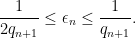
then the residual errors  are positive reals, which initially take the values

and evolve according to the recursion

when  (rightward shift case), or

when  (upward shift case). (Note that the border case
  does not occur when is irrational.) In particular we see that the
  and
and  decrease monotonically to zero.
We may now justify the terminology of best rational approximation:
Proposition 1 (Best rational approximation)Let  , and let be the last basis in the semiconvergent basis sequence for which
  . Then for any natural numbers
  and
and  , one has

and

or
and

Proof: As form a basis for , we have
for some integers  ; in particular,

This already gives the claim when  and
and  , or when
  and
and  . The case
  cannot occur since this would make
  , so we are left with the case
  . But in this case, we have
  , and hence
  by construction, again a contradiction.
We can also track the dynamics of the semiconvergent basis sequence by introducing the relative slope  of with respect to the cone , defined as the unique positive real number such that
As is irrational, the  are all irrational. It is not difficult to see that the are defined by the following recursion:
  , and one has
  when
when  , and
, and  when
when  . Also, the former case arises when
  is the upward shift of , and the latter case arises when we have a rightward shift instead.
The semiconvergent basis sequence can be viewed as a sequence of  upward shifts for some non-negative integer , followed by
  rightward shifts for some positive integer , then
  upward shifts for some positive integer , and so forth. By tracking what happens to the relative slope and its reciprocal
  , we conclude that

for some  ,
,

for some  , and so forth, leading to the familiar continued fraction expansion

We recursively define the sequence  of lattice vectors by the formulae

and

for  , thus


etc. We may then describe the bases in terms of the  as follows: if

for some  and , then one has

if  is even, and

if is odd. In particular, the sequence of bases contains the sequence

as a subsequence, representing the places is the sequence in which one changes from a rightward shift to an upward shift or vice versa. In particular, if  , then the slopes
  (known as successive convergents to ) converge to from below when is even, and from above when is odd. As bases have determinant
  , we also see that

By construction, we have the recurrences
and
with initial conditions  and
and  , thus


etc. From an induction we see that the  are a monotonically increasing sequence of natural numbers. Indeed, they must increase at least as fast as the Fibonacci sequence
  ; from an easy induction we see that
  ,
,  for all
  . In particular, the
  must grow at least exponentially fast in .
As with the basis sequence , we can express the in the  basis:

or equivalently

Then the  are positive reals, with
  ,
,  , and
, and

By construction, we see that the are monotone decreasing in for ; indeed, we see that are essentially the output of the Euclidean algorithm applied to the real numbers  . From (1)we see that
Since  and
and  for , we see in particular that
In particular we have a fairly precise description of how well the convergents approximate :
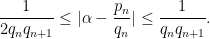
In particular, we have

As the are best rational approximants, we thus also have

whenever  .
.
Remark 1 From the above inequalities one can easily establish the Dirichlet approximation theorem and the (one-dimensional) Kronecker approximation theorem.
— 2. Bohr sets —
Now we compare rank one Bohr sets to rank two progressions  . It turns out that the best progressions to use here come from using the denominators
  of a semiconvergent basis as the generators. Indeed, if

then we have

and

Thus we have

whenever

In the converse direction, suppose that  , thus
  and one has
  for some integer
  . As is a basis for , we have
for some integers . Taking wedge products, we see that

We write  for some
  , and similarly write
  for
for  , to conclude that

and similarly

We conclude that

whenever

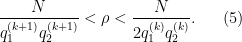
It is now a routine matter to optimise the parameters  to obtain a good fit. Suppose for instance that
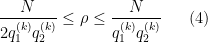
for some  . If we then set

then we have

Also, since is a basis, we have  , and thus

In particular,


We thus conclude from the preceding discussion that

On the other hand, we have

and similarly

and thus by the preceding discussion

and similarly

Thus, in this case, the rank one Bohr set is morally the same object (up to constants) as the rank two progression  .
.
Things are a bit more complicated in the regime
For sake of discussion, let us suppose that is an upward shift of , so that  and
and  . From (5) we see that
  and hence
  . Also, we have
  , so in particular,
 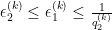 . If we now set
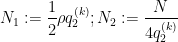
then we have

and


and so
Conversely, we have


while


and so once again we have
and
Thus again we see that in this case is morally the same object as  .
.
Note that as shrinks, the lengths shrink also, though every so often there is a discontinuity when  is incremented, thus shearing the generators as well as the lengths . (Technically, there is also a discontinuity when one passes from (4) to (5), but this is an artificial discontinuity and can be eliminated by performing a smoother interpolation between these two regimes which we omit.) Among other things, the above relationships give a rough description of the cardinality of the Bohr set ; one has

and thus (by unifying all the cases) one has

whenever

It is a shame that there is no similarly precise formula known for the size of a rank two Bohr set  , as this would likely lead (among other things) to a resolution of the Littlewood conjecture.
— 3. A reformulation of the Littlewood conjecture —
The Littlewood conjecture asserts that for any two real numbers  , one has

The conjecture remains open, although there are some highly non-trivial partial results, such as the result of Einsiedler, Katok, and Lindenstrauss that the set of pairs  for which the Littlewood conjecture fails is so small that it has Hausdorff dimension zero.
If a pair was a counterexample to the Littlewood conjecture, then

for all positive integers . In particular, one has

for all (in other words, is badly approximable by rationals, and is in particular irrational). Applying (2), we conclude that  for all , or equivalently that the coefficients
  of the continued fraction expansion of are bounded. (Conversely, using (2) and (3) we see that if is irrational with bounded continued fraction coefficients, then it is badly approximable by rationals.) Similarly for
  . This is already enough to establish without much additional work that the Littlewood conjecture is true for almost all (in the sense of Lebesgue measure), although it does not come close to the stronger result of Einseidler, Katok, and Lindenstrauss mentioned above (it is known that the set of badly approximable numbers has Hausdorff dimension one).
One can reformulate the Littlewood conjecture in terms of the denominators  of the convergents to , and the denominators
  of the convergents to :
Proposition 2 Let be two real numbers. Then the following are equivalent:
Recall that a progression  is said to be proper if all of the elements
  ,
,  of the progression are distinct.
Proof: Let us first show that (i) implies (ii). Let be a counterexample to the Littlewood conjecture, thus

for all non-zero integers . We have already seen that are badly approximable (so in particular and  . Now let
  be a sufficiently small number, and suppose that the progression (6) is not proper for some
  . Then there is a non-trivial solution to the equation

for some integers  , not all zero, with
  and
and  . Let be the integer in (8), then is non-zero and
  . Also, from (2) we see that

and similarly
and thus

Setting  small enough, we contradict (7).
Now we show that (ii) implies (i). Let  be as in (ii). Suppose for contradiction that (i) fails, thus we can find a sequence
  of integers going off to infinity such that

where  denotes a quantity that goes to zero as (or
  ) goes to infinity. In particular, one can find
  (depending on ) such that

(Indeed, one can pick  to be
to be  and to be
  .) As the
  increase in a lacunary fashion (thanks to the bad approximability of ), we can find such that
  ; similarly we may find
  such that
  , thus


Thus lies in the Bohr sets

and

Applying the analysis of the preceding section, we conclude that lies in the rank two progressions

and

and is non-zero, and so the rank four progression

is not proper. But this contradicts (ii) for large enough.
We can now give a heuristic explanation as to why there should not be any counterexample to the Littlewood conjecture. Such a counterexample can be completely described by the continued fraction coefficients  for , and the continued fraction coefficients
  for . These sequences need to be bounded by the bad approximability property; let us suppose that they are both bounded by some bound
  . Thus, for any
  , the number of choices for
  and
and  grows at most exponentially in (it is about
  ). Of course, these coefficients then determine the denominators
  and
and  by the recurrences given previously.
On the other hand, by the above proposition, there needs to be an such that for each  and
and  , the progression (6) is proper. We can heuristically gauge how likely this occurs by the following numerology. For fixed (and making the non-degeneracy assumptions that
  ), there are about
  different ways to form a sum of the form

with and  . These sums have magnitude about
  . Thus, we expect that the probability that all non-trivial sums avoid zero (which is basically what is needed for (6) to be proper) to be at most
  for some
  depending only on .
On the other hand, the number of eligible pairs  for which the progression (6) is non-degenerate enough to have a chance of being proper grows quadratically in . Due to the exponential growth of and
  , it is reasonable to suppose that the properness of each of the progressions (6) behave like independent (or at least very weakly coupled) events as vary (viewing
  and as being drawn uniformly from all sequences bounded by ). If we assume that this independence is so strong as to be like joint independence (and here is where we really make a serious leap of faith), then we therefore expect the probability that a randomly chosen choice of coefficients has all of the (6) proper should decay quadratic-exponentially in (i.e. it should be something like
  , particularly if we choose
  and
and  to be comparable in magnitude). As this beats the entropy of for large enough, we thus expect that for any given
  , there should not in fact be any counterexamples to (ii) (and hence to the Littlewood conjecture) with this choice of parameters.
This heuristic derivation of the Littlewood conjecture uses a common (but highly nonrigorous) probabilistic argument, in which one argues that there are so many ways in which a candidate can fail to be a counterexample to the conjecture that no counterexample actually exists. This type of heuristic is common in number theory, for instance justifying the even Goldbach conjecture (for sufficiently large even numbers, at least). Unfortunately, we do not know how to rule out the existence of some bizarre “conspiracy” between the coefficients and  that manage to align all the possible (and supposedly independent) failure events in such a way that an extremely lucky and exceptional choice of coefficients manages to evade all of these events and end up as a counterexample to the conjecture. But the best we can do with current technology is to show that such conspiracies, if they exist at all, are very rare (with the aforementioned result of Einsiedler, Katok, and Lindenstrauss being the strongest result currently known of this type).

.


15 comments
Comments feed for this article
5 January, 2012 at 9:10 am
US.Alkalinewater@yahoo.com
The heuristic derivation of the Littlewood conjecture seems quite probable to me.
9 January, 2012 at 6:34 pm
anonymous
Small typo in section 1 ( ,
,  ).
).
Many thanks for the heuristic derivation. The EKL paper is difficult to get through without a background in the subject.
[Corrected, thanks – T.]
10 January, 2012 at 4:44 am
petequinn
In case anyone is interested in coverage of continued fractions accessible to the layperson, Manfred Schroeder covers some interesting aspects of the topic in two books, “Fractals, Chaos, Power Laws,” (Dover) and “Number Theory in Science and Communication,” (Springer).
10 January, 2012 at 7:09 am
mathfromhell
I am going to have to research this topic….thanks for the detailed discourse…
26 January, 2012 at 4:28 pm
windfarmmusic
Fantastic! I was hoping to find just such a discussion of continued fractions which starts from the geometrical viewpoint.
Do you have any insight on how the analysis might change if instead of Bohr sets as you’ve defined them, one considered an ‘inhomogenous’ version
with an additional parameter ?
?
29 March, 2017 at 8:46 pm
Sam Chow
I discuss this in arXiv:1703.07016.
10 March, 2012 at 8:27 am
Ułamki łańcuchowe – cz 3. Moja macierzowa reprezentacja « FIKSACJE
[…] ( po szczegóły odsyłam czytelnika do wcześniejszego wpisu – oraz polecam niedawny wpis na blogu Terrence Tao – w którym przedstawiono w abstrakcyjnej profesjonalnej notacji wyniki opublikowane – chyba […]
17 March, 2012 at 9:27 am
kazekkurz
I was playing with continued fractions and obtain probably interesting algebraic representation of it, and interesting algebraic structure within. maybe some of You will be interested…
Here are the citation:
“In this workbook I will show matrix representation of continued fractions (CF) different from typical one. In typical representation, two matrix L, and R are used. On the Stern-Brocot tree ( SBTree) representation of CF, matrix R decodes move to the right child and L move to the left child of given SBTree node. We may call it RL representation of CF.
Representation below gives other, complementary picture, where matrix S means “reverse direction” whilst matrix T means “go step forward”.I will call it S(ST) representation for the reasons which will be explained below. ”
It seems that these two ways of decoding walk on tree, exhaust the all the simple, canonical, natural, I do not know how to name it, ways to decode every possible walks on binary tree. Only the first, RL representation I have found in literature of the subject. Maybe this second one is only a curiosity, but maybe it would be interesting for someone.
For x- real number, represented as continued fraction with continuant matrix 2×2 – M (similar to returned in Pari/GP by contfracpnqn([a0,a1…an]) function) I have obtain interesting formula:
Where matrices S, T and L are defined in sage workbook below. requirement det(M) = +-1 is represented as equation for quadratic curve in certain ring over rational numbers. Please find details below.
Here is a page on my blog with links to Sage notebook with explanations:
Here is worksheet itself on sagenb server: http://sagenb.com/home/pub/4535/
Sorry for the spam…
I have hope I am not terribly wrong…
Best regards
Kazimierz Kurz
18 March, 2012 at 12:34 am
kazekkurz
One additional remark – interesting part of the formula above is that it is independent from the basis choice ( because of trace cyclic property, You may use any base system by linear similarity transformation and then change matrices S,T,L and M within it ) and then function from continuant matrices to continued fractions space is interesting. If You look at t closer You wil find that both nominator ( tr(M(S-L)) and denominator ( tr(M(S-T)) are just continuant polynomials – but in closed form – you may differentiate them, add, multiply etc. In Graham, Knuth Patashnik You may find a section about continuant polynomials, and they obeys many recurrence equations – any of them is a consequence of “noncommutativity” of product which appears in M definition M = S*prod(S*(ST)^{a_i}). As far as I know – no such formula is described in literature of the subject – I check a lot of articles and books looking for something similar. Please note, that in decomposed form (M = a*I+b*S+c*T+d*L – You may find definition of this objects in Sage workbook) this formula is also linear in a,b,c,d – so it may be interesting from numerical point of view…
13 April, 2012 at 3:35 pm
peteg
I think there’s a typo in the Continued Fraction section, in the expression for when
when  . It should be
  .
.
[Corrected, thanks. (I presume you mean instead of
  . -T.]
14 April, 2012 at 3:12 pm
Ryan Reich
In the proof of Proposition 1, I think you want to consider and not
  .
.
[Corrected, thanks – T.]
22 April, 2012 at 4:16 pm
peteg
I think there’s a typo in the 4’th element of the sequence of pairs of ‘s . It should be
  not
not  . [Corrected, thanks – T.]
18 May, 2012 at 3:50 pm
meditationatae
Dear Professor Tao,
I’m truly intrigued by your Proposition 2.1 and your probabilistic argument
for the Littlewood conjecture. Using $M$ and $\epsilon$ as in your
heuristic argument, I’ve been wondering if it’s conceivable that the
probabilistic argument could be “extended” in some sense to give
an order of magnitude estimate (based on heuristics, probabilistic
assumptions) for the (smallest) positive integer $N(M, \epsilon)$ having
the property: for all $\alpha$, $\beta$ in $R/Z$,
min_{1 <= n <= $N(M, \epsilon)$ } n || n $\alpha$ || || n $\beta$ || < $\epsilon$ , given the fixed parameter values $M$ and $\epsilon$ .
Thanks.
18 May, 2012 at 3:58 pm
meditationatae
[edit: added latex keyword …]
Dear Professor Tao,
I’m truly intrigued by your Proposition 2.1 and your probabilistic argument
for the Littlewood conjecture. Using $latexM$ and $latex\epsilon$ as in your
heuristic argument, I’ve been wondering if it’s conceivable that the
probabilistic argument could be “extended” in some sense to give
an order of magnitude estimate (based on heuristics, probabilistic
assumptions) for the (smallest) positive integer $latexN(M, \epsilon)$ having
the property: for all $latex\alpha$, $latex\beta$ in $latexR/Z$,
min_{1 leq n leq $latexN(M, \epsilon)$ } n || n $latex\alpha$ || || n $latex\beta$ || lt $latex\epsilon$ , given the fixed parameter values $latexM$ and $latex\epsilon$ .
Thanks.
30 March, 2015 at 12:50 pm
254A, Notes 8: The Hardy-Littlewood circle method and Vinogradov’s theorem | What's new
[…] sharper estimates here by using the classical theory of continued fractions and Bohr sets, as in this previous blog post, but we will not need these refinements […]