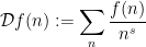
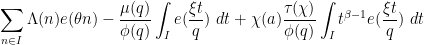
We have seen in previous notes that the operation of forming a Dirichlet series

\displaystyle  {\mathcal D} f(n) := \sum_n \frac{f(n)}{n^s}

or twisted Dirichlet series

\displaystyle  {\mathcal D} \chi f(n) := \sum_n \frac{f(n) \chi(n)}{n^s}

is an incredibly useful tool for questions in multiplicative number theory. Such series can be viewed as a multiplicative Fourier transform, since the functions {n \mapsto \frac{1}{n^s}} and {n \mapsto \frac{\chi(n)}{n^s}} are multiplicative characters.
Similarly, it turns out that the operation of forming an additive Fourier series

\displaystyle  \hat f(\theta) := \sum_n f(n) e(-n \theta),

where {\theta} lies on the (additive) unit circle {{\bf R}/{\bf Z}} and {e(\theta) := e^{2\pi i \theta}} is the standard additive character, is an incredibly useful tool for additive number theory, particularly when studying additive problems involving three or more variables taking values in sets such as the primes; the deployment of this tool is generally known as the Hardy-Littlewood circle method. (In the analytic number theory literature, the minus sign in the phase {e(-n\theta)} is traditionally omitted, and what is denoted by {\hat f(\theta)} here would be referred to instead by {S_f(-\theta)}, {S(f;-\theta)} or just {S(-\theta)}.) We list some of the most classical problems in this area:

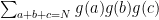
  • (Even Goldbach conjecture) Is it true that every even natural number {N} greater than two can be expressed as the sum {p_1+p_2} of two primes?
  • (Odd Goldbach conjecture) Is it true that every odd natural number {N} greater than five can be expressed as the sum {p_1+p_2+p_3} of three primes?
  • (Waring problem) For each natural number {k}, what is the least natural number {g(k)} such that every natural number {N} can be expressed as the sum of {g(k)} or fewer {k^{th}} powers?
  • (Asymptotic Waring problem) For each natural number {k}, what is the least natural number {G(k)} such that every sufficiently large natural number {N} can be expressed as the sum of {G(k)} or fewer {k^{th}} powers?
  • (Partition function problem) For any natural number {N}, let {p(N)} denote the number of representations of {N} of the form {N = n_1 + \dots + n_k} where {k} and {n_1 \geq \dots \geq n_k} are natural numbers. What is the asymptotic behaviour of {p(N)} as {N \rightarrow \infty}?

The Waring problem and its asymptotic version will not be discussed further here, save to note that the Vinogradov mean value theorem (Theorem 13 from Notes 5) and its variants are particularly useful for getting good bounds on {G(k)}; see for instance the ICM article of Wooley for recent progress on these problems. Similarly, the partition function problem was the original motivation of Hardy and Littlewood in introducing the circle method, but we will not discuss it further here; see e.g. Chapter 20 of Iwaniec-Kowalski for a treatment.

Instead, we will focus our attention on the odd Goldbach conjecture as our model problem. (The even Goldbach conjecture, which involves only two variables instead of three, is unfortunately not amenable to a circle method approach for a variety of reasons, unless the statement is replaced with something weaker, such as an averaged statement; see this previous blog post for further discussion. On the other hand, the methods here can obtain weaker versions of the even Goldbach conjecture, such as showing that “almost all” even numbers are the sum of two primes; see Exercise 34 below.) In particular, we will establish the following celebrated theorem of Vinogradov:

Theorem 1 (Vinogradov’s theorem) Every sufficiently large odd number {N} is expressible as the sum of three primes.

Recently, the restriction that {n} be sufficiently large was replaced by Helfgott with {N > 5}, thus establishing the odd Goldbach conjecture in full. This argument followed the same basic approach as Vinogradov (based on the circle method), but with various estimates replaced by “log-free” versions (analogous to the log-free zero-density theorems in Notes 7), combined with careful numerical optimisation of constants and also some numerical work on the even Goldbach problem and on the generalised Riemann hypothesis. We refer the reader to Helfgott’s text for details.

We will in fact show the more precise statement:

Theorem 2 (Quantitative Vinogradov theorem) Let {N \geq 2} be an natural number. Then

\displaystyle  \sum_{a,b,c: a+b+c=N} \Lambda(a) \Lambda(b) \Lambda(c) = G_3(N) \frac{N^2}{2} + O_A( N^2 \log^{-A} N )

for any {A>0}, where

\displaystyle  G_3(N) = \prod_{p|N} (1-\frac{1}{(p-1)^2}) \times \prod_{p \not | N} (1 + \frac{1}{(p-1)^3}). \ \ \ \ \ (1)

The implied constants are ineffective.

We dropped the hypothesis that {N} is odd in Theorem 2, but note that {G_3(N)} vanishes when {N} is even. For odd {N}, we have

\displaystyle  1 \ll G_3(N) \ll 1.

Exercise 3 Show that Theorem 2 implies Theorem 1.

Unfortunately, due to the ineffectivity of the constants in Theorem 2 (a consequence of the reliance on the Siegel-Walfisz theorem in the proof of that theorem), one cannot quantify explicitly what “sufficiently large” means in Theorem 1 directly from Theorem 2. However, there is a modification of this theorem which gives effective bounds; see Exercise 32 below.

Exercise 4 Obtain a heuristic derivation of the main term {G_3(N) \frac{N^2}{2}} using the modified Cramér model (Section 1 of Supplement 4).

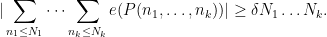
To prove Theorem 2, we consider the more general problem of estimating sums of the form

\displaystyle  \sum_{a,b,c \in {\bf Z}: a+b+c=N} f(a) g(b) h(c)

for various integers {N} and functions {f,g,h: {\bf Z} \rightarrow {\bf C}}, which we will take to be finitely supported to avoid issues of convergence.
Suppose that {f,g,h} are supported on {\{1,\dots,N\}}; for simplicity, let us first assume the pointwise bound {|f(n)|, |g(n)|, |h(n)| \ll 1} for all {n}. (This simple case will not cover the case in Theorem 2, when {f,g,h} are truncated versions of the von Mangoldt function {\Lambda}, but will serve as a warmup to that case.) Then we have the trivial upper bound

\displaystyle  \sum_{a,b,c \in {\bf Z}: a+b+c=N} f(a) g(b) h(c) \ll N^2. \ \ \ \ \ (2)


A basic observation is that this upper bound is attainable if {f,g,h} all “pretend” to behave like the same additive character {n \mapsto e(\theta n)} for some {\theta \in {\bf R}/{\bf Z}}. For instance, if {f(n)=g(n)=h(n) = e(\theta n) 1_{n \leq N}}, then we have {f(a)g(b)h(c) = e(\theta N)} when {a+b+c=N}, and then it is not difficult to show that

\displaystyle  \sum_{a,b,c \in {\bf Z}: a+b+c=N} f(a) g(b) h(c) = (\frac{1}{2}+o(1)) e(\theta N) N^2

as {N \rightarrow \infty}.
The key to the success of the circle method lies in the converse of the above statement: the only way that the trivial upper bound (2) comes close to being sharp is when {f,g,h} all correlate with the same character {n \mapsto e(\theta n)}, or in other words {\hat f(\theta), \hat g(\theta), \hat h(\theta)} are simultaneously large. This converse is largely captured by the following two identities:

Exercise 5 Let {f,g,h: {\bf Z} \rightarrow {\bf C}} be finitely supported functions. Then for any natural number {N}, show that

\displaystyle  \sum_{a,b,c: a+b+c=N} f(a) g(b) h(c) = \int_{{\bf R}/{\bf Z}} \hat f(\theta) \hat g(\theta) \hat h(\theta) e(\theta N)\ d\theta \ \ \ \ \ (3)

and

\displaystyle  \sum_n |f(n)|^2 = \int_{{\bf R}/{\bf Z}} |\hat f(\theta)|^2\ d\theta.

The traditional approach to using the circle method to compute sums such as {\sum_{a,b,c: a+b+c=N} f(a) g(b) h(c)} proceeds by invoking (3) to express this sum as an integral over the unit circle, then dividing the unit circle into “major arcs” where {\hat f(\theta), \hat g(\theta),\hat h(\theta)} are large but computable with high precision, and “minor arcs” where one has estimates to ensure that {\hat f(\theta), \hat g(\theta),\hat h(\theta)} are small in both {L^\infty} and {L^2} senses. For functions {f,g,h} of number-theoretic significance, such as truncated von Mangoldt functions, the “major arcs” typically consist of those {\theta} that are close to a rational number {\frac{a}{q}} with {q} not too large, and the “minor arcs” consist of the remaining portions of the circle. One then obtains lower bounds on the contributions of the major arcs, and upper bounds on the contribution of the minor arcs, in order to get good lower bounds on {\sum_{a,b,c: a+b+c=N} f(a) g(b) h(c)}.

This traditional approach is covered in many places, such as this text of Vaughan. We will emphasise in this set of notes a slightly different perspective on the circle method, coming from recent developments in additive combinatorics; this approach does not quite give the sharpest quantitative estimates, but it allows for easier generalisation to more combinatorial contexts, for instance when replacing the primes by dense subsets of the primes, or replacing the equation {a+b+c=N} with some other equation or system of equations.

From Exercise 5 and Hölder’s inequality, we immediately obtain

Corollary 6 Let {f,g,h: {\bf Z} \rightarrow {\bf C}} be finitely supported functions. Then for any natural number {N}, we have

\displaystyle  |\sum_{a,b,c: a+b+c=N} f(a) g(b) h(c)| \leq (\sum_n |f(n)|^2)^{1/2} (\sum_n |g(n)|^2)^{1/2}

\displaystyle  \times \sup_\theta |\sum_n h(n) e(n\theta)|.

Similarly for permutations of the {f,g,h}.

In the case when {f,g,h} are supported on {[1,N]} and bounded by {O(1)}, this corollary tells us that we have {\sum_{a,b,c: a+b+c=N} f(a) g(b) h(c)} is {o(N^2)} whenever one has {\sum_n h(n) e(n\theta) = o(N)} uniformly in {\theta}, and similarly for permutations of {f,g,h}. From this and the triangle inequality, we obtain the following conclusion: if {f} is supported on {[1,N]} and bounded by {O(1)}, and {f} is Fourier-approximated by another function {g} supported on {[1,N]} and bounded by {O(1)} in the sense that

\displaystyle  \sum_n f(n) e(n\theta) = \sum_n g(n) e(n\theta) + o(N)

uniformly in {\theta}, then we have

\displaystyle  \sum_{a,b,c: a+b+c=N} f(a) f(b) f(c) = \sum_{a,b,c: a+b+c=N} g(a) g(b) g(c) + o(N^2). \ \ \ \ \ (4)

Thus, one possible strategy for estimating the sum {\sum_{a,b,c: a+b+c=N} f(a) f(b) f(c)} is, one can effectively replace (or “model”) {f} by a simpler function {g} which Fourier-approximates {g} in the sense that the exponential sums {\sum_n f(n) e(n\theta), \sum_n g(n) e(n\theta)} agree up to error {o(N)}. For instance:

Exercise 7 Let {N} be a natural number, and let {A} be a random subset of {\{1,\dots,N\}}, chosen so that each {n \in \{1,\dots,N\}} has an independent probability of {1/2} of lying in {A}.

  • (i) If {f := 1_A} and {g := \frac{1}{2} 1_{[1,N]}}, show that with probability {1-o(1)} as {N \rightarrow \infty}, one has {\sum_n f(n) e(n\theta) = \sum_n g(n) e(n\theta) + o(N)} uniformly in {\theta}. (Hint: for any fixed {\theta}, this can be accomplished with quite a good probability (e.g. {1-o(N^{-2})}) using a concentration of measure inequality, such as Hoeffding’s inequality. To obtain the uniformity in {\theta}, round {\theta} to the nearest multiple of (say) {1/N^2} and apply the union bound).
  • (ii) Show that with probability {1-o(1)}, one has {(\frac{1}{16}+o(1))N^2} representations of the form {N=a+b+c} with {a,b,c \in A} (with {(a,b,c)} treated as an ordered triple, rather than an unordered one).

In the case when {f} is something like the truncated von Mangoldt function {\Lambda(n) 1_{n \leq N}}, the quantity {\sum_n |f(n)|^2} is of size {O( N \log N)} rather than {O( N )}. This costs us a logarithmic factor in the above analysis, however we can still conclude that we have the approximation (4) whenever {g} is another sequence with {\sum_n |g(n)|^2 \ll N \log N} such that one has the improved Fourier approximation

\displaystyle  \sum_n f(n) e(n\theta) = \sum_n g(n) e(n\theta) + o(\frac{N}{\log N}) \ \ \ \ \ (5)


uniformly in {\theta}. (Later on we will obtain a “log-free” version of this implication in which one does not need to gain a factor of {\frac{1}{\log N}} in the error term.)
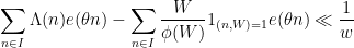
This suggests a strategy for proving Vinogradov’s theorem: find an approximant {g} to some suitable truncation {f} of the von Mangoldt function (e.g. {f(n) = \Lambda(n) 1_{n \leq N}} or {f(n) = \Lambda(n) \eta(n/N)}) which obeys the Fourier approximation property (5), and such that the expression {\sum_{a+b+c=N} g(a) g(b) g(c)} is easily computable. It turns out that there are a number of good options for such an approximant {g}. One of the quickest ways to obtain such an approximation (which is used in Chapter 19 of Iwaniec and Kowalski) is to start with the standard identity {\Lambda = -\mu L * 1}, that is to say

\displaystyle  \Lambda(n) = - \sum_{d|n} \mu(d) \log d,

and obtain an approximation by truncating {d} to be less than some threshold {R} (which, in practice, would be a small power of {N}):

\displaystyle  \Lambda(n) \approx - \sum_{d \leq R: d|n} \mu(d) \log d. \ \ \ \ \ (6)

Thus, for instance, if {f(n) = \Lambda(n) 1_{n \leq N}}, the approximant {g} would be taken to be

\displaystyle  g(n) := - \sum_{d \leq R: d|n} \mu(d) \log d 1_{n \leq N}.

One could also use the slightly smoother approximation

\displaystyle  \Lambda(n) \approx \sum_{d \leq R: d|n} \mu(d) \log \frac{R}{d} \ \ \ \ \ (7)

in which case we would take

\displaystyle  g(n) := \sum_{d \leq R: d|n} \mu(d) \log \frac{R}{d} 1_{n \leq N}.

The function {g} is somewhat similar to the continuous Selberg sieve weights studied in Notes 4, with the main difference being that we did not square the divisor sum as we will not need to take {g} to be non-negative. As long as {z} is not too large, one can use some sieve-like computations to compute expressions like {\sum_{a+b+c=N} g(a)g(b)g(c)} quite accurately. The approximation (5) can be justified by using a nice estimate of Davenport that exemplifies the Mobius pseudorandomness heuristic from Supplement 4:

Theorem 8 (Davenport’s estimate) For any {A>0} and {x \geq 2}, we have

\displaystyle  \sum_{n \leq x} \mu(n) e(\theta n) \ll_A x \log^{-A} x

uniformly for all {\theta \in {\bf R}/{\bf Z}}. The implied constants are ineffective.

This estimate will be proven by splitting into two cases. In the “major arc” case when {\theta} is close to a rational {a/q} with {q} small (of size {O(\log^{O(1)} x)} or so), this estimate will be a consequence of the Siegel-Walfisz theorem ( from Notes 2); it is the application of this theorem that is responsible for the ineffective constants. In the remaining “minor arc” case, one proceeds by using a combinatorial identity (such as Vaughan’s identity) to express the sum {\sum_{n \leq x} \mu(n) e(\theta n)} in terms of bilinear sums of the form {\sum_n \sum_m a_n b_m e(\theta nm)}, and use the Cauchy-Schwarz inequality and the minor arc nature of {\theta} to obtain a gain in this case. This will all be done below the fold. We will also use (a rigorous version of) the approximation (6) (or (7)) to establish Vinogradov’s theorem.

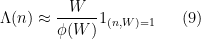
A somewhat different looking approximation for the von Mangoldt function that also turns out to be quite useful is

\displaystyle  \Lambda(n) \approx \sum_{q \leq Q} \sum_{a \in ({\bf Z}/q{\bf Z})^\times} \frac{\mu(q)}{\phi(q)} e( \frac{an}{q} ) \ \ \ \ \ (8)


for some {Q} that is not too large compared to {N}. The methods used to establish Theorem 8 can also establish a Fourier approximation that makes (8) precise, and which can yield an alternate proof of Vinogradov’s theorem; this will be done below the fold.
The approximation (8) can be written in a way that makes it more similar to (7):

Exercise 9 Show that the right-hand side of (8) can be rewritten as

\displaystyle  \sum_{d \leq Q: d|n} \mu(d) \rho_d

where

\displaystyle  \rho_d := \frac{d}{\phi(d)} \sum_{m \leq Q/d: (m,d)=1} \frac{\mu^2(m)}{\phi(m)}.

Then, show the inequalities

\displaystyle  \sum_{m \leq Q/d} \frac{\mu^2(m)}{\phi(m)} \leq \rho_d \leq \sum_{m \leq Q} \frac{\mu^2(m)}{\phi(m)}

and conclude that

\displaystyle  \log \frac{Q}{d} - O(1) \leq \rho_d \leq \log Q + O(1).

(Hint: for the latter estimate, use Theorem 27 of Notes 1.)

The coefficients {\rho_d} in the above exercise are quite similar to optimised Selberg sieve coefficients (see Section 2 of Notes 4).

Another approximation to {\Lambda}, related to the modified Cramér random model (see Model 10 of Supplement 4) is

\displaystyle  \Lambda(n) \approx \frac{W}{\phi(W)} 1_{(n,W)=1} \ \ \ \ \ (9)


where {W := \prod_{p \leq w} p} and {w} is a slowly growing function of {N} (e.g. {w = \log\log N}); a closely related approximation is

\displaystyle  \frac{\phi(W)}{W} \Lambda(Wn+b) \approx 1 \ \ \ \ \ (10)

for {W,w} as above and {1 \leq b \leq W} coprime to {W}. These approximations (closely related to a device known as the “{W}-trick”) are not as quantitatively accurate as the previous approximations, but can still suffice to establish Vinogradov’s theorem, and also to count many other linear patterns in the primes or subsets of the primes (particularly if one injects some additional tools from additive combinatorics, and specifically the inverse conjecture for the Gowers uniformity norms); see this paper of Ben Green and myself for more discussion (and this more recent paper of Shao for an analysis of this approach in the context of Vinogradov-type theorems). The following exercise expresses the approximation (9) in a form similar to the previous approximation (8):

Exercise 10 With {W} as above, show that

\displaystyle  \frac{W}{\phi(W)} 1_{(n,W)=1} = \sum_{q|W} \sum_{a \in ({\bf Z}/q{\bf Z})^\times} \frac{\mu(q)}{\phi(q)} e( \frac{an}{q} )

for all natural numbers {n}.

— 1. Exponential sums over primes: the minor arc case —

We begin by developing some simple rigorous instances of the following general heuristic principle (cf. Section 3 of Supplement 4):

Principle 11 (Equidistribution principle) An exponential sum (such as a linear sum {\sum_n e(f(n))} or a bilinear sum {\sum_n \sum_m a_n b_m e(f(n,m))} involving a “structured” phase function {f} should exhibit some non-trivial cancellation, unless there is an “obvious” algebraic reason why such cancellation may not occur (e.g. {f} is approximately periodic with small period, or {f(n,m)} approximately decouples into a sum {g(n)+h(m)}).

There are some quite sophisticated versions of this principle in the literature, such as Ratner’s theorems on equidistribution of unipotent flows, discussed in this previous blog post. There are yet further precise instances of this principle which are conjectured to be true, but for which this remains unproven (e.g. regarding incomplete Weil sums in finite fields). Here, though, we will focus only on the simplest manifestations of this principle, in which {f} is a linear or bilinear phase. Rigorous versions of this special case of the above principle will be very useful in estimating exponential sums such as

\displaystyle  \sum_{n \leq x} \Lambda(n) e(\theta n)

or

\displaystyle  \sum_{n \leq x} \mu(n) e(\theta n)

in “minor arc” situations in which {\theta} is not too close to a rational number {a/q} of small denominator. The remaining “major arc” case when {\theta} is close to such a rational number {a/q} has to be handled by the complementary methods of multiplicative number theory, which we turn to later in this section.
For pedagogical reasons we shall develop versions of this principle that are in contrapositive form, starting with a hypothesis that a significant bias in an exponential sum is present, and deducing algebraic structure as a consequence. This leads to estimates that are not fully optimal from a quantitative viewpoint, but I believe they give a good qualitative illustration of the phenomena being exploited here.

We begin with the simplest instance of Principle 11, namely regarding unweighted linear sums of linear phases:

Lemma 12 Let {I \subset {\bf Z}} be an interval of length at most {N} for some {N \geq 1}, let {\theta \in{\bf R}/{\bf Z}}, and let {\delta > 0}.

  • (i) If

    \displaystyle  |\sum_{n \in I} e(\theta n)| \geq \delta N,

    Then {\|\theta\|_{{\bf R}/{\bf Z}} \ll \frac{1}{\delta N}}, where {\|\theta\|_{{\bf R}/{\bf Z}}} denotes the distance from (any representative of) {\theta} to the nearest integer.

  • (ii) More generally, if

    \displaystyle  |\sum_{n \in I} f(n) e(\theta n)| > \delta N \sup_{n \in I} |f(n)|

    for some monotone function {f: I \rightarrow {\bf R}}, then {\|\theta\|_{{\bf R}/{\bf Z}} \ll \frac{1}{\delta N}}.

Proof: From the geometric series formula we have

\displaystyle  |\sum_{n \in I} e(\theta n)| \leq \frac{2}{|e(\theta)-1|} \ll \frac{1}{\|\theta\|_{{\bf R}/{\bf Z}}}

and the claim (i) follows. To prove (ii), we write {I = \{a,\dots,b\}} and observe from summation by parts that

\displaystyle  \sum_{n \in I} f(n) e(\theta n) = f(a) \sum_{n \in I} e(\theta n) + \sum_{m = a+1}^b (f(m)-f(m-1)) \sum_{n=m}^b e(\theta n)

while from monotonicity we have

\displaystyle  |f(a)|+ \sum_{m = a+1}^b |f(m)-f(m-1)| \leq 2 \sup_{n \in I} |f(n)|

and the claim then follows from (i) and the pigeonhole principle. \Box
Now we move to bilinear sums. We first need an elementary lemma:

Lemma 13 (Vinogradov lemma) Let {I \subset {\bf Z}} be an interval of length at most {N} for some {N \geq 1}, and let {\theta \in{\bf R}/{\bf Z}} be such that {\|n\theta\|_{{\bf R}/{\bf Z}} \leq \varepsilon} for at least {\delta N} values of {n \in I}, for some {0 < \varepsilon, \delta < 1}. Then either

\displaystyle  N < \frac{2}{\delta}

or

\displaystyle  \varepsilon > 10^{-2} \delta

or else there is a natural number {q \leq 2/\delta} such that

\displaystyle  \| q \theta \|_{{\bf R}/{\bf Z}} \ll \frac{\varepsilon}{\delta N}.

One can obtain somewhat sharper estimates here by using the classical theory of continued fractions and Bohr sets, as in this previous blog post, but we will not need these refinements here.

Proof: We may assume that {N \geq \frac{2}{\delta}} and {\varepsilon \leq 10^{-2} \delta}, since we are done otherwise. Then there are at least two {n \in I} with {\|n \theta \|_{{\bf R}/{\bf Z}} \leq \varepsilon}, and by the pigeonhole principle we can find {n_1 < n_2} in {I} with {\|n_1 \theta \|_{{\bf R}/{\bf Z}}, \|n_2 \theta \|_{{\bf R}/{\bf Z}} \leq \varepsilon} and {n_2-n_1 \leq \frac{2}{\delta}}. By the triangle inequality, we conclude that there exists at least one natural number {q \leq \frac{2}{\delta}} for which

\displaystyle  \| q \theta \|_{{\bf R}/{\bf Z}} \leq 2\varepsilon.

We take {q} to be minimal amongst all such natural numbers, then we see that there exists {a} coprime to {q} and {|\kappa| \leq 2\varepsilon} such that

\displaystyle  \theta = \frac{a}{q} + \frac{\kappa}{q}. \ \ \ \ \ (11)


If {\kappa=0} then we are done, so suppose that {\kappa \neq 0}. Suppose that {n < m} are elements of {I} such that {\|n\theta \|_{{\bf R}/{\bf Z}}, \|m\theta \|_{{\bf R}/{\bf Z}} \leq \varepsilon} and {m-n \leq \frac{1}{10 \kappa}}. Writing {m-n = qk + r} for some {0 \leq r < q}, we have

\displaystyle  \| (m-n) \theta \|_{{\bf R}/{\bf Z}} = \| \frac{ra}{q} + (m-n) \frac{\kappa}{q} \|_{{\bf R}/{\bf Z}} \leq 2\varepsilon.

By hypothesis, {(m-n) \frac{\kappa}{q} \leq \frac{1}{10 q}}; note that as {q \leq 2/\delta} and {\varepsilon \leq 10^{-2} \delta} we also have {\varepsilon \leq \frac{1}{10q}}. This implies that {\| \frac{ra}{q} \|_{{\bf R}/{\bf Z}} < \frac{1}{q}} and thus {r=0}. We then have

\displaystyle  |k \kappa| \leq 2 \varepsilon.

We conclude that for fixed {n \in I} with {\|n\theta \|_{{\bf R}/{\bf Z}} \leq \varepsilon}, there are at most {\frac{2\varepsilon}{|\kappa|}} elements {m} of {[n, n + \frac{1}{10 |\kappa|}]} such that {\|m\theta \|_{{\bf R}/{\bf Z}} \leq \varepsilon}. Iterating this with a greedy algorithm, we see that the number of {n \in I} with {\|n\theta \|_{{\bf R}/{\bf Z}} \leq \varepsilon} is at most {(\frac{N}{1/10|\kappa|} + 1) 2\varepsilon/|\kappa|}; since {\varepsilon < 10^{-2} \delta}, this implies that

\displaystyle  \delta N \ll 2 \varepsilon / \kappa

and the claim follows. \Box
Now we can control bilinear sums of the form

\displaystyle  \sum_{n \in I} \alpha*\beta(n) e(\theta n) = \sum_{m,n: mn\in I} \alpha(m) \beta(n) e(\theta nm).

Theorem 14 (Bilinear sum estimate) Let {M, N \geq 1}, let {I \subset {\bf Z}} be an interval, and let {a: {\bf N} \rightarrow {\bf C}}, {\beta: {\bf N} \rightarrow {\bf C}} be sequences supported on {[1,M]} and {[1,N]} respectively. Let {\delta > 0} and {\theta \in {\bf R}/{\bf Z}}.

  • (i) (Type I estimate) If {\beta} is real-valued and monotone and

    \displaystyle  |\sum_{m,n: mn \in I} \alpha(m) \beta(n) e( \theta nm )| > \delta MN \sup_m |\alpha(m)| \sup_n |\beta(n)|

    then either {N \ll \delta^{-2}}, or there exists {q \ll 1/\delta} such that {\|q\theta\|_{{\bf R}/{\bf Z}} \ll \frac{1}{\delta^2 NM}}.

  • (ii) (Type II estimate) If

    \displaystyle  |\sum_{m,n: mn \in I} \alpha(m) \beta(n) e( \theta nm )| > \delta (MN)^{1/2}

    \displaystyle  \times (\sum_m |\alpha(m)|^2)^{1/2} (\sum_n |\beta(n)|^2)^{1/2}

    then either {\min(M,N) \ll \delta^{-4}}, or there exists {q \ll 1/\delta^2} such that {\|q\theta\|_{{\bf R}/{\bf Z}} \ll \frac{1}{\delta^4 NM}}.

The hypotheses of (i) and (ii) should be compared with the trivial bounds

\displaystyle  |\sum_{m,n: mn \in I} \alpha(m) \beta(n) e( \theta nm )| \leq MN \sup_m |\alpha(m)| \sup_n |\beta(n)|

and

\displaystyle  |\sum_{m,n: mn \in I} \alpha(m) \beta(n) e( \theta nm )| \leq (MN)^{1/2} (\sum_m |\alpha(m)|^2)^{1/2} (\sum_n |\beta(n)|^2)^{1/2}

arising from the triangle inequality and the Cauchy-Schwarz inequality.
Proof: We begin with (i). By the triangle inequality, we have

\displaystyle  \sum_{m \leq M} |\sum_{n: mn \in I} \beta(n) e( \theta nm )| > \delta MN \sup_n |\beta(n)|.

The summand in {m} is bounded by {N \sup_n |\beta(n)|}. We conclude that

\displaystyle  |\sum_{n: mn \in I} \beta(n) e( \theta nm )| > \frac{\delta}{2} N \sup_n |\beta(n)|

for at least {\frac{\delta}{2} M} choices of {m \leq M} (this is easiest to see by arguing by contradiction). Applying Lemma 12(ii), we conclude that

\displaystyle  \| \theta m \|_{{\bf R}/{\bf Z}} \ll \frac{1}{\delta N} \ \ \ \ \ (12)

for at least {\frac{\delta}{2} M} choices of {m \leq M}. Applying Lemma 13, we conclude that one of {M \ll 1/\delta}, {\frac{1}{\delta N} \gg \delta}, or there exists a natural number {q \ll 1/\delta} such that {\|q\theta \|_{{\bf R}/{\bf Z}} \ll \frac{1}{\delta^2 NM}}. This gives (i) except when {M \ll 1/\delta}. In this case, we return to (12), which holds for at least one natural number {m \leq M \ll 1/\delta}, and set {q := m}.
Now we prove (ii). By the triangle inequality, we have

\displaystyle  \sum_m |\alpha(m)| |\sum_{n: mn \in I} \beta(n) e( \theta nm )|

\displaystyle  > \delta (MN)^{1/2} (\sum_m |\alpha(m)|^2)^{1/2} (\sum_n |\beta(n)|^2)^{1/2}

and hence by the Cauchy-Schwarz inequality

\displaystyle  \sum_{m\leq M} |\sum_{n: mn \in I} \beta(n) e( \theta nm )|^2 > \delta^2 MN \sum_n |\beta(n)|^2.

The left-hand side expands as

\displaystyle  \sum_{n,n' \leq N} \beta(n) \overline{\beta(n')} \sum_{m \leq M: mn, mn' \in I} e(\theta(n-n') m);

from the triangle inequality, the estimate {\beta(n) \overline{\beta(n')} \ll |\beta(n)|^2 + |\beta(n')|^2} and symmetry we conclude that

\displaystyle  \sum_{n \leq N} |\sum_{m \leq M: mn, mn' \in I} e(\theta(n-n') m)| \gg \delta^2 M N

for at least one choice of {n' \leq N}. Fix this {n'}. Since {|\sum_{m \leq M: mn, mn' \in I} e(\theta(n-n') m)| \leq M}, we thus have

\displaystyle  |\sum_{m \leq M: mn, mn' \in I} e(\theta(n-n') m)| \gg \delta^2 M

for {\gg \delta^2 N} choices of {n \leq N}. Applying Lemma 12(i), we conclude that

\displaystyle  \| \theta(n-n') \|_{{\bf R}/{\bf Z}} \ll \frac{1}{\delta^2 M }

for {\gg \delta^2 N} choices of {n \leq N}. Applying Lemma 13, we obtain the claim. \Box
The following exercise demonstrates the sharpness of the above theorem, at least with regards to the bound on {q}.

Exercise 15 Let {\frac{a}{q}} be a rational number with {(a,q)=1}, let {\theta \in {\bf R}/{\bf Z}}, and let {M, N} be multiples of {q}.

  • (i) If {\|\theta - \frac{a}{q}\|_{{\bf R}/{\bf Z}} \leq \frac{c}{qNM}} for a sufficiently small absolute constant {c>0}, show that {|\sum_{n \leq N} \sum_{m \leq M} e( \theta nm ) | \gg \frac{1}{q} NM}.
  • (ii) If {a} is even, and {\|\theta - \frac{a}{q}\|_{{\bf R}/{\bf Z}} \leq \frac{c}{\sqrt{q}NM}} for a sufficiently small absolute constant {c>0}, show that {|\sum_{n \leq N} \sum_{m \leq M} e( a n^2/2q) e(-a m^2/2q) e( \theta nm ) | \gg \frac{1}{\sqrt{q}} NM}.

Exercise 16 (Quantitative Weyl exponential sum estimates) Let {P(n) = \alpha_d n^d + \dots + \alpha_1 n + \alpha_0} be a polynomial with coefficients {\alpha_0,\dots,\alpha_d \in {\bf R}/{\bf Z}} for some {d \geq 1}, let {N \geq 1}, and let {\delta > 0}.

  • (i) Suppose that {|\sum_{n \in I} e(P(n))| \geq \delta N} for some interval {I} of length at most {N}. Show that there exists a natural number {q \ll_d \delta^{-O_d(1)}} such that {\| q\alpha_d \|_{{\bf R}/{\bf Z}} \ll_d \delta^{-O_d(1)} / N^d}. (Hint: induct on {d} and use the van der Corput inequality (Proposition 7 of Notes 5).
  • (ii) Suppose that {|\sum_{n \in I} e(P(n))| \geq \delta N} for some interval {I} contained in {[1,N]}. Show that there exists a natural number {q \ll_d \delta^{-O_d(1)}} such that {\| q\alpha_j \|_{{\bf R}/{\bf Z}} \ll_d \delta^{-O_d(1)} / N^j} for all {0 \leq j \leq d} (note this claim is trivial for {j=0}). (Hint: use downwards induction on {j}, adjusting {q} as one goes along, and split up {I} into somewhat short arithmetic progressions of various spacings {q} in order to turn the top degree components of {P(n)} into essentially constant phases.)
  • (iii) Use these bounds to give an alternate proof of Exercise 8 of Notes 5.

We remark that sharper versions of the above exercise are available if one uses the Vinogradov mean value theorem from Notes 5; see Theorem 1.6 of this paper of Wooley.

Exercise 17 (Quantitative multidimensional Weyl exponential sum estimates) Let {P(n_1,\dots,n_k) = \sum_{i_1+\dots+i_k \leq d} \alpha_{i_1,\dots,i_k} n_1^{i_1} \dots n_k^{i_k}} be a polynomial in {k} variables with coefficients {\alpha_{i_1,\dots,i_k} \in {\bf R}/{\bf Z}} for some {d \geq 1}. Let {N_1,\dots,N_k \geq 1} and {\delta > 0}. Suppose that

\displaystyle  |\sum_{n_1 \leq N_1} \dots \sum_{n_k \leq N_k} e( P(n_1,\dots,n_k) )| \geq \delta N_1 \dots N_k.

Show that either one has {N_j \ll_{d,k} \delta^{-O_{d,k}(1)}} for some {j=1,\dots,k}, or else there exists a natural number {q \ll_{d,k} \delta^{-O_{d,k}(1)}} such that {\|q \alpha_{i_1,\dots,i_k} \|_{{\bf R}/{\bf Z}} \ll \frac{\delta^{-O_{d,k}(1)}}{N_1^{i_1} \dots N_k^{i_k}}} for all {i_1,\dots,i_k}. (Note: this is a rather tricky exercise, and is only recommended for students who have mastered the arguments needed to solve the one-dimensional version of this exercise from Exercise 16. A solution is given in this blog post.)

Recall that in the proof of the Bombieri-Vinogradov theorem (see Notes 3), sums such as {\sum_n \Lambda(n) \chi(n)} or {\sum_n \mu(n) \chi(n)} were handled by using combinatorial identities such as Vaughan’s identity to split {\Lambda} or {\mu} into combinations of Type I or Type II convolutions. The same strategy can be applied here:

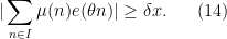
Proposition 18 (Minor arc exponential sums are small) Let {x \geq 2}, {\delta > 0}, and {\theta \in {\bf R}/{\bf Z}}, and let {I} be an interval in {[1,x]}. Suppose that either

\displaystyle  |\sum_{n\in I} \Lambda(n) e(\theta n)| \geq \delta x \ \ \ \ \ (13)

or

\displaystyle  |\sum_{n\in I} \mu(n) e(\theta n)| \geq \delta x. \ \ \ \ \ (14)

Then either {x \ll \delta^{-O(1)}}, or there exists a natural number {q \ll \delta^{-2} \log^{O(1)} x} such that {\| q \theta \|_{{\bf R}/{\bf Z}} \ll \delta^{-5} \frac{\log^{O(1)} x}{x}}.

The exponent in the bound {x \ll \delta^{-O(1)}} can be made explicit (and fairly small) if desired, but this exponent is not of critical importance in applications. The losses of {\log x} in this proposition are undesirable (though affordable, for the purposes of proving results such as Vinogradov’s theorem); these losses have been reduced over the years, and finally eliminated entirely in the recent work of Helfgott.

Proof: We will prove this under the hypothesis (13); the argument for (14) is similar and is left as an exercise. By removing the portion of {I} in {[0, \delta x/2]}, and shrinking {\delta} slightly, we may assume without loss of generality that {I \subset [\delta x, x]}.

We recall the Vaughan identity

\displaystyle  \Lambda = \Lambda_{\leq V} + \mu_{\leq U} * L - \mu_{\leq U} * \Lambda_{\leq V} * 1 + \mu_{>U} * \Lambda_{>V} * 1

valid for any {U,V > 1}; see Lemma 18 of Notes 3. We select {U=V=x^{1/3}}. By the triangle inequality, one of the assertions

\displaystyle  |\sum_{n\in I} \Lambda_{\leq V}(n) e(\theta n)| \gg \delta x \ \ \ \ \ (15)

\displaystyle  |\sum_{n\in I} \mu_{\leq U} * L(n) e(\theta n)| \gg \delta x \ \ \ \ \ (16)

\displaystyle  |\sum_{n\in I} \mu_{\leq U} * \Lambda_{\leq V} * 1(n) e(\theta n)| \gg \delta x \ \ \ \ \ (17)

\displaystyle  |\sum_{n\in I} \mu_{>U} * \Lambda_{>V} * 1(n) e(\theta n)| \gg \delta x \ \ \ \ \ (18)

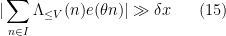
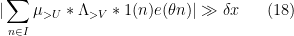
must hold. If (15) holds, then {V \gg \delta x}, from which we easily conclude that {x \ll \delta^{-O(1)}}. Now suppose that (16) holds. By dyadic decomposition, we then have

\displaystyle  |\sum_{n\in I} \alpha * \beta(n) e(\theta n)| \gg \frac{\delta x}{\log^{O(1)} x} \ \ \ \ \ (19)

where {\alpha, \beta} are restrictions of {\mu_{\leq U}}, {L} to dyadic intervals {[M,2M]}, {[N,2N]} respectively. Note that the location of {I} then forces {\delta x \ll MN \ll x}, and the support of {\mu_{\leq U}} forces {M \ll U}, so that {N \gg x/U = x^{2/3}}. Applying Theorem 14(i), we conclude that either {N \ll \delta^{-2} \log^{O(1)} x} (and hence {x \ll \delta^{-O(1)}}), or else there is {q \ll \delta^{-2} \log^{O(1)} x} such that {\| q \theta \|_{{\bf R}/{\bf Z}} \ll \delta^{-3} \frac{\log^{O(1)} x}{x}}, and we are done.
Similarly, if (17) holds, we again apply dyadic decomposition to arrive at (19), where {\alpha,\beta} are now restrictions of {\mu_{\leq U} * \Lambda_{\leq V}} and {1} to {[M,2M]} and {[N,2N]}. As before, we have {\delta x \ll MN \ll x}, and now {M \ll UV} and so {N \gg x^{1/3}}. Note from the identity {\sum_{d|n} \Lambda(d)=\log n} that {\alpha} is bounded pointwise by {\log x}. Repeating the previous argument then gives one of the required conclusions.

Finally, we consider the “Type II” scenario in which (18) holds. We again dyadically decompose and arrive at (19), where {\alpha} and {\beta} are now the restrictions of {\mu_{>U}} and {\Lambda_{>V}*1} (say) to {[M,2M]} and {[N,2N]}, so that {\delta x \ll MN \ll x}, {M \gg U}, and {N \gg V}. As before we can bound {\beta} pointwise by {\log x}. Applying Theorem 14(ii), we conclude that either {\min(M,N) \ll \delta^{-4} \log^{O(1)} x}, or else there exists {q \ll \delta^{-2} \log^{O(1)} x} such that {\|q\theta\|_{{\bf R}/{\bf Z}} \ll \delta^{-5} \frac{\log^{O(1)} x}{x}}, and we again obtain one of the desired conclusions. \Box

Exercise 19 Finish the proof of Proposition 18 by treating the case when (14) occurs.

Exercise 20 Establish a version of Proposition 18 in which (13) or (14) are replaced with

\displaystyle  |\sum_{p \leq x} e( \theta p )| \gg \delta \frac{x}{\log x}.

— 2. Exponential sums over primes: the major arc case —

Proposition 18 provides guarantees that exponential sums such as {\sum_{n \leq x} \Lambda(n) e(\theta n)} are much smaller than {x}, unless {x} is itself small, or if {\theta} is close to a rational number {a/q} of small denominator. We now analyse this latter case. In contrast with the minor arc analysis, the implied constants will usually be ineffective.

The situation is simplest in the case of the Möbius function:

Proposition 21 Let {I} be an interval in {[1,x]} for some {x \geq 2}, and let {\theta \in {\bf R}/{\bf Z}}. Then for any {A>0} and natural number {q}, we have

\displaystyle  \sum_{n \in I} \mu(n) e(\theta n) \ll_A (q + x \| q \theta \|_{{\bf R}/{\bf Z}}) x \log^{-A} x.

The implied constants are ineffective.

Proof: By splitting into residue classes modulo {q}, it suffices to show that

\displaystyle  \sum_{n \in I: n = a\ (q)} \mu(n) e(\theta n) \ll_A (1 + \frac{x}{q} \| q \theta \|_{{\bf R}/{\bf Z}}) x \log^{-A} x

for all {a = 0,\dots,q-1}. Writing {n = qm+a}, and removing a factor of {e(a\theta)}, it suffices to show that

\displaystyle  \sum_{m \in {\bf Z}: qm+a \in I} \mu(qm+a) e(\xi m) \ll_A (1 + \frac{x}{q} \| q \theta \|_{{\bf R}/{\bf Z}}) x \log^{-A} x

where {\xi \in {\bf R}} is the representative of {q\theta} that is closest to the origin, so that {|\xi| = \|q\theta\|_{{\bf R}/{\bf Z}}}.
For all {m} in the above sum, one has {0 \leq m \leq x/q}. From the fundamental theorem of calculus, one has

\displaystyle  e(\xi m) = 1 + 2\pi i \xi \int_0^{x/q} e(\xi t) 1_{m \geq t}\ dt \ \ \ \ \ (20)


and so by the triangle inequality it suffices to show that

\displaystyle  \sum_{m \in {\bf Z}: qm+a \in I; m \geq t} \mu(qm+a) \ll_A x \log^{-A} x

for all {0 \leq t \leq x/q}. But this follows from the Siegel-Walfisz theorem for the Möbius function (Exercise 66 of Notes 2). \Box
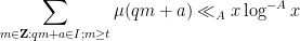
Arguing as in the proof of Lemma 12(ii), we also obtain the corollary

\displaystyle  \sum_{n \in I} \mu(n) e(\theta n) f(n) \ll_A (q + x \| q \theta \|_{{\bf R}/{\bf Z}}) x \log^{-A} x \sup_{n \in I} |f(n)| \ \ \ \ \ (21)


for any monotone function {f: I \rightarrow {\bf R}}, with ineffective constants.
Davenport’s theorem (Theorem 8) is now immediate from applying Proposition 18 with {\delta := \log^{-A} x}, followed by Proposition 21 (with {A} replaced by a larger constant) to deal with the major arc case.

Now we turn to the analogous situation for the von Mangoldt function {\Lambda}. Here we expect to have a non-trivial main term in the major arc case: for instance, the prime number theorem tells us that {\sum_{n \leq I} \Lambda(n) e(\theta n)} should be approximately the length of {I} when {\theta=0}. There are several ways to describe the behaviour of {\Lambda}. One way is to use the approximation

\displaystyle  \Lambda^\sharp_R(n) := - \sum_{d \leq R: d|n} \mu(d) \log d

discussed in the introduction:
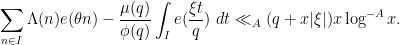
Proposition 22 Let {x \geq 2} and let {R} be such that {R \geq x^\varepsilon}. Then for any interval {I} in {[1,x]} and any {\theta \in {\bf R}/{\bf Z}}, one has

\displaystyle  \sum_{n \in I} \Lambda(n) e(\theta n) - \sum_{n \in I} \Lambda^\sharp_R(n) e(\theta n) \ll_{A,\varepsilon} x \log^{-A} x \ \ \ \ \ (22)

for all {A>0}. The implied constants are ineffective.

Proof: As discussed in the introduction, we have

\displaystyle  \Lambda(n) - \Lambda^\sharp_R(n) = - \sum_{d>R: d|n} \mu(d) \log d

so the left-hand side of (22) can be rearranged as

\displaystyle  - \sum_m \sum_{d>R: dm \in I} \mu(d) \log d e( m \theta d).

Since {I \subset [1,x]}, the inner sum vanishes unless {m \leq x/R}. From Theorem 8 and summation by parts (or (21) and Proposition 21), we have

\displaystyle  \sum_{d>R: dm \in I} \mu(d) \log d e( m \theta d) \ll_A \frac{x}{m} \log^{-A}(x/m) \times \log x;

since {m \leq x/R}, we have {\log^{-A}(x/m) \ll_{A,\varepsilon} \log^{-A} x}, and the claim now follows from summing in {m} (and increasing {A} appropriately). \Box

Exercise 23 Show that Proposition 22 continues to hold if {\Lambda^\sharp_R} is replaced by the function

\displaystyle  \Lambda_R(n) := \sum_{d \leq R: d|n} \mu(d) \log \frac{R}{d}

or more generally by

\displaystyle  \Lambda_{R,\eta}(n) := \log R \sum_{d \leq R: d|n} \mu(d) \eta( \frac{\log d}{\log R} )

where {\eta: {\bf R} \rightarrow {\bf R}} is a bounded function such that {\eta(t) = 1-t} for {0 \leq t \leq 1/2} and {\eta(t)=0} for {t>1}. (Hint: use a suitable linear combination of the identities {\Lambda = - \mu L * 1} and {\Lambda = \mu * L}.)

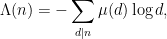
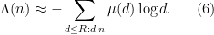
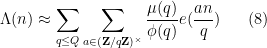
Alternatively, we can try to replicate the proof of Proposition 21 directly, keeping track of the main terms that are now present in the Siegel-Walfisz theorem. This gives a quite explicit approximation for {\sum_{n \in I} \Lambda(n) e(\theta n)} in major arc cases:

Proposition 24 Let {I} be an interval in {[1,x]} for some {x \geq 2}, and let {\theta \in {\bf R}/{\bf Z}} be of the form {\theta = \frac{a}{q} + \frac{\xi}{q}}, where {q \geq 1} is a natural number, {a \in ({\bf Z}/q{\bf Z})^\times}, and {\xi \in {\bf R}}. Then for any {A>0}, we have

\displaystyle  \sum_{n \in I} \Lambda(n) e(\theta n) - \frac{\mu(q)}{\phi(q)} \int_I e(\frac{\xi t}{q})\ dt \ll_A (q + x |\xi|) x \log^{-A} x.

The implied constants are ineffective.

Proof: We may assume that {|\xi| \leq \frac{\log^{A} x}{x}} and {q \leq \log^A x}, as the claim follows from the triangle inequality and the prime number theorem otherwise. For similar reasons we can also assume that {x} is sufficiently large depending on {A}.

As in the proof of Proposition 21, we decompose into residue classes mod {q} to write

\displaystyle  \sum_{n \in I} \Lambda(n) e(\theta n) = \sum_{b \in {\bf Z}/q{\bf Z}} \sum_{n \in I: n = b\ (q)} \Lambda(n) e(\theta n).

If {b} is not coprime to {q}, then one easily verifies that

\displaystyle  \sum_{n \in I: n = b\ (q)} \Lambda(n) e(\theta n) \ll \log^2 x

and the contribution of these cases is thus acceptable. Thus, up to negligible errors, we may restrict {b} to be coprime to {q}. Writing {n = qm+b}, we thus may replace {\sum_{n \in I} \Lambda(n) e(\theta n)} by

\displaystyle  \sum_{b \in ({\bf Z}/q{\bf Z})^\times} e(\theta b) \sum_{m: qm+b \in I} \Lambda(qm+b) e(\xi m).

Applying (20), we can write

\displaystyle  \sum_{m: qm+b \in I} \Lambda(qm+b) e(\xi m) = \sum_{m: qm+b \in I} \Lambda(qm+b)

\displaystyle + 2\pi i \xi \int_0^{x/q} e(\xi t) \sum_{m: qm+b \in I; m \geq t} \Lambda(qm+b)\ dt.

Applying the Siegel-Walfisz theorem (Exercise 64 of Notes 2), we can replace {\Lambda} here by {\frac{q}{\phi(q)}}, up to an acceptable error. Applying (20) again, we have now replaced {\sum_{n \in I} \Lambda(n) e(\theta n)} by

\displaystyle  \frac{q}{\phi(q)} \sum_{b \in ({\bf Z}/q{\bf Z})^\times} e(\theta b) \sum_{m: qm+b \in I} e(\xi m),

which we can rewrite as

\displaystyle  \frac{q}{\phi(q)} \sum_{n \in I: (n,q)=1} e(\theta n).

From Möbius inversion one has

\displaystyle  1_{(n,q)=1} = \sum_{d|q} \mu(d) 1_{d|n},

so we can rewrite the previous expression as

\displaystyle  \frac{q}{\phi(q)} \sum_{d|q} \mu(d) \sum_{m: dm \in I} e(d\theta m).

For {d|q} with {d < q}, we see from the hypotheses that {\|d\theta\|_{{\bf R}/{\bf Z}} \gg 1/q}, and so {\sum_{m: dm \in I} e(d\theta m) \ll q} by Lemma 12(i). The contribution of all {d<q} is then {\ll \frac{q}{\phi(q)} \tau(q) q}, which is acceptable since {q \leq \log^A x}. So, up to acceptable errors, we may replace {\sum_{n \in I} \Lambda(n) e(\theta n)} by {\frac{q}{\phi(q)} \mu(q) \sum_{m: qm \in I} e(q\theta m)}. We can write {e(q\theta m)=e(\xi m)}, and the claim now follows from Exercise 11 of Notes 1 and a change of variables. \Box

Exercise 25 Assuming the generalised Riemann hypothesis, obtain the significantly stronger estimate

\displaystyle  \sum_{n \in I} \Lambda(n) e(\theta n) - \frac{\mu(q)}{\phi(q)} \int_I e(\frac{\xi t}{q})\ dt \ll (q + x |\xi|)^{O(1)} x^{1/2} \log^2 x

with effective constants. (Hint: use Exercise 48 of Notes 2, and adjust the arguments used to prove Proposition 24 accordingly.)

Exercise 26 If {q \leq \log^A x} and there is a real primitive Dirichlet character {\chi} of modulus {q} whose {L}-function {L(\cdot,\chi)} has an exceptional zero {\beta} with {1 - \frac{c}{\log q} \leq \beta < 1} for a sufficiently small {c}, establish the variant

\displaystyle  \sum_{n \in I} \Lambda(n) e(\theta n) - \frac{\mu(q)}{\phi(q)} \int_I e(\frac{\xi t}{q})\ dt + \chi(a) \frac{\tau(\chi)}{\phi(q)} \int_I t^{\beta-1} e(\frac{\xi t}{q})\ dt

\displaystyle \ll_A (q + x |\xi|) x \log^{-A} x

of Proposition 24, with the implied constants now effective and with the Gauss sum {\tau(\chi)} defined in equation (11) of Supplement 2. If there is no such primitive Dirichlet character, show that the above estimate continues to hold with the exceptional term {\overline{\chi(a)} \frac{\tau(\chi)}{\phi(q)} \int_I t^{\beta-1} e(\frac{\xi t}{q})\ dt} deleted.

Informally, the above exercise suggests that one should add an additional correction term {- \frac{q}{\phi(q)} \chi(n) n^{\beta-1}} to the model for {\Lambda} when there is an exceptional zero.

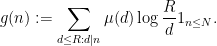
We can now formalise the approximation (8):

Exercise 27 Let {A > 0}, and suppose that {B} is sufficiently large depending on {A}. Let {x \geq 2}, and let {Q} be a quantity with {\log^B x \leq Q \leq x^{1/2} \log^{-B} x}. Let {\nu_Q: {\bf N} \rightarrow {\bf R}} be the function

\displaystyle  \nu_Q(n) := \sum_{q \leq Q} \sum_{a \in ({\bf Z}/q{\bf Z})^\times} \frac{\mu(q)}{\phi(q)} e( \frac{an}{q} ).

Show that for any interval {I \subset [1,x]}, we have

\displaystyle  \sum_{n \in I} \Lambda(n) e(\theta n) - \sum_{n \in I} \nu_Q(n) e(\theta n) \ll_A x \log^{-A} x

for all {\theta \in {\bf R}/{\bf Z}}, with ineffective constants.

We also can formalise the approximations (9), (10):

Exercise 28 Let {x \geq 2}, and let {w > 1} be such that {w \leq \frac{1}{4} \log x}. Write {W := \prod_{p \leq w} p}.

  • (i) Show that

    \displaystyle  \sum_{n \in I} \Lambda(n) e(\theta n) - \sum_{n \in I} \frac{W}{\phi(W)} 1_{(n,W)=1} e(\theta n) \ll \frac{1}{w}

    for all {\theta \in {\bf R}/{\bf Z}} and {I \subset [1,x]}, with an ineffective constant.

  • (ii) Suppose now that {x \geq 100} and {w = O(\log\log x)}. Let {1 \leq b \leq W} be coprime to {W}, and let {\Lambda_{b,W} := \frac{\phi(W)}{W} \Lambda(Wn+b)}. Show that

    \displaystyle  \sum_{n \in I} \Lambda_b(n) e(\theta n) - \sum_{n \in I} e(\theta n) \ll \frac{1}{w}

    for all {\theta \in {\bf R}/{\bf Z}} and {I \subset [1,x]}.

Proposition 24 suggests that the exponential sum {\sum_{n \in I} \Lambda(n) e(\theta n)} should be of size about {x / \phi(q)} when {\theta} is close to {a/q} and {q} is fairly small, and {x} is large. However, the arguments in Proposition 18 only give an upper bound of {O( x / \sqrt{q} )} instead (ignoring logarithmic factors). There is a good reason for this discrepancy, though. The proof of Proposition 24 relied on the Siegel-Walfisz theorem, which in turn relied on Siegel’s theorem. As discussed in Notes 2, the bounds arising from this theorem are ineffective – we do not have any control on how the implied constant in the estimate in Proposition 24 depends on {A}. In contrast, the upper bounds in Proposition 18 are completely effective. Furthermore, these bounds are close to sharp in the hypothetical scenario of a Landau-Siegel zero:

Exercise 29 Let {c} be a sufficiently small (effective) absolute constant. Suppose there is a non-principal character {\chi} of conductor {q} with an exceptional zero {\beta \geq 1 - \frac{c}{\log q}}. Let {x \geq 2} be such that {q \leq \exp(c \sqrt{\log x} )} and {\beta \geq 1 - \frac{c}{\log x}}. Show that

\displaystyle  |\sum_{n \leq x} \Lambda(n) e( \frac{a}{q} n )| \gg \frac{x \sqrt{q}}{\phi(q)} \geq \frac{x}{\sqrt{q}}

for every {a \in ({\bf Z}/q{\bf Z})^\times}.

This exercise indicates that apart from the factors of {\log x}, any substantial improvements to Proposition 18 will first require some progress on the notorious Landau-Siegel zero problem. It also indicates that if a Landau-Siegel zero is present, then one way to proceed is to simply incorporate the effect of that zero into the estimates (so that the computations for major arc exponential sums would acquire an additional main term coming from the exceptional zero), and try to establish results like Vinogradov’s theorem separately in this case (similar to how things were handled for Linnik’s theorem, see Notes 7), by using something like Exercise 26 in place of Proposition 24.

— 3. Vinogradov’s theorem —

We now have a number of routes to establishing Theorem 2. Let {N} be a large number. We wish to compute the expression

\displaystyle  \sum_{a,b,c \in {\bf N}: a+b+c=N} \Lambda(a) \Lambda(b) \Lambda(c)

or equivalently

\displaystyle  \sum_{a,b,c \in {\bf Z}: a+b+c=N} f(a) f(b) f(c)

where {f(n) := \Lambda(n) 1_{1 \leq n \leq N}}.
Now we replace {f} by a more tractable approximation {g}. There are a number of choices for {g} that were presented in the previous section. For sake of illustration, let us select the choice

\displaystyle  g(n) := \log R \sum_{d \leq R: d|n} \mu(d) \eta( \frac{\log d}{\log R} ) 1_{1 \leq n\leq N} \ \ \ \ \ (23)


where {R := N^{1/10}} (say) and where {\eta: {\bf R} \rightarrow {\bf R}} is a fixed smooth function supported on {[-1,1]} such that {\eta(t) = 1-t} for {0 \leq t \leq 1/2}. From Exercise 23 we have

\displaystyle  \sup_{\theta \in {\bf R}/{\bf Z}} | \sum_n (f(n)-g(n)) e(n \theta) | \ll_{A,\eta} N \log^{-A} N

(with ineffective constants) for any {A>0}. Also, by bounding {g} by the divisor function on {[1,N]} we have the bounds

\displaystyle  \sum_n |f(n)|^2, \sum_n |g(n)|^2 \ll N \log^{O(1)} N

so from several applications of Corollary 6 (splitting {f} as the sum of {f-g} and {g}) we have

\displaystyle  \sum_{a,b,c \in {\bf Z}: a+b+c=N} f(a) f(b) f(c) =

\displaystyle  \sum_{a,b,c \in {\bf Z}: a+b+c=N} g(a) g(b) g(c) + O_A( N^2 \log^{-A} N )

for any {A>0} (again with ineffective constants).
Now we compute {\sum_{a,b,c \in {\bf Z}: a+b+c=N} g(a) g(b) g(c)}. Using (23), we may rearrange this expression as

\displaystyle  \log^3 R \sum_{d_1,d_2,d_3} (\prod_{i=1}^3 \mu(d_i) \eta(\frac{\log d_i}{\log R})) \sum_{a,b,c \in {\bf N}: d_1|a, d_2|b, d_3|c, a+b+c=N} 1.

The inner sum can be estimated by covering the {(a,b)} parameter space by squares of sidelength {[d_1, d_2, d_3]} (the least common multiple of {d_1,d_2,d_3}) as

\displaystyle  \sum_{a,b,c \in {\bf N}: d_1|a, d_2|b, d_3|c, a+b+c=N} 1 = \rho(d_1,d_2,d_3) \frac{N^2}{2} + O( N d_1 d_2 d_3 )

where {\rho(d_1,d_2,d_3)} is the proportion of residue classes in the plane {\{ (a,b,c) \in ({\bf Z}/[d_1,d_2,d_3]): a+b+c=N\ ([d_1,d_2,d_3])\}} with {d_1|a, d_2|b, d_3|c}. Since {d_1,d_2,d_3 \leq R = N^{1/10}}, the contribution of the error term is certainly acceptable, so

\displaystyle  \sum_{a,b,c \in {\bf Z}: a+b+c=N} f(a) f(b) f(c)

\displaystyle  = \frac{N^2}{2} \log^3 R \sum_{d_1,d_2,d_3} (\prod_{i=1}^3 \mu(d_i) \eta(\frac{\log d_i}{\log R})) \rho(d_1,d_2,d_3) + O_A( N^2 \log^{-A} N).

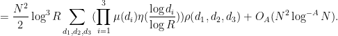
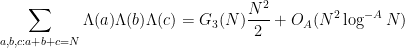
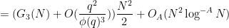
Thus to prove Theorem 2, it suffices to establish the asymptotic

\displaystyle  \log^3 R \sum_{d_1,d_2,d_3} (\prod_{i=1}^3 \mu(d_i) \eta(\frac{\log d_i}{\log R})) \rho(d_1,d_2,d_3) = G_3(N) + O_A( \log^{-A} N ). \ \ \ \ \ (24)

From the Chinese remainder theorem we see that {\rho} is multiplicative in the sense that {\rho(d_1 d'_1,d_2 d'_2, d_3 d'_3) = \rho(d_1,d_2,d_3) \rho(d'_1,d'_2,d'_3)} when {d_1d_2d_3} is coprime to {d'_1d'_2d'_3}, so to evaluate this quantity for squarefree {d_1,d_2,d_3} it suffices to do so when {d_1,d_2,d_3 \in \{1,p\}} for a single prime {p}. This is easily done:

Exercise 30 Show that

\displaystyle  \rho(d_1,d_2,d_3) = \frac{1}{d_1 d_2 d_3}

except when {d_1=d_2=d_3=p}, in which case one has

\displaystyle  \rho(p,p,p) = \frac{1_{p|N}}{p^2}.

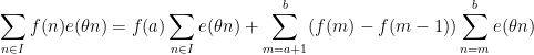
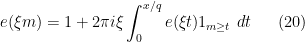
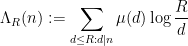
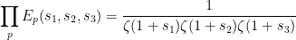
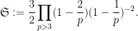
The left-hand side of (24) is an expression similar to that studied in Section 2 of Notes 4, and can be estimated in a similar fashion. Namely, we can perform a Fourier expansion

\displaystyle  e^u \eta( u ) = \int_{\bf R} F(t) e^{-itu}\ dt \ \ \ \ \ (25)


for some smooth, rapidly decreasing {F: {\bf R} \rightarrow {\bf C}}. This lets us write the left-hand side of (24) as

\displaystyle  \log^3 R \int_{\bf R} \int_{\bf R} \int_{\bf R} \sum_{d_1,d_2,d_3} \frac{\mu(d_1) \mu(d_2) \mu(d_3) \rho(d_1,d_2,d_3)}{d_1^{(1+it_1)/\log R} d_2^{(1+it_2)/\log R} d_3^{(1+it_3)/\log R}}

\displaystyle  F(t_1) F(t_2) F(t_3)\ dt_1 dt_2 dt_3.

We can factor this as

\displaystyle  \log^3 R \int_{\bf R} \int_{\bf R} \int_{\bf R} \prod_p E_p(\frac{1+it_1}{\log R},\frac{1+it_2}{\log R},\frac{1+it_3}{\log R}) \ \ \ \ \ (26)

\displaystyle  F(t_1) F(t_2) F(t_3)\ dt_1 dt_2 dt_3

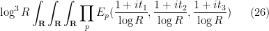
where (by Exercise 30)

\displaystyle  E_p(s_1,s_2,s_3) = 1 - \frac{1}{p^{1+s_1}} - \frac{1}{p^{1+s_2}} - \frac{1}{p^{1+s_3}}

\displaystyle  + \frac{1}{p^{2+s_1+s_2}} + \frac{1}{p^{2+s_1+s_3}} + \frac{1}{p^{2+s_2+s_3}}

\displaystyle  - \frac{1_{p|N}}{p^{2+s_1+s_2+s_3}}.

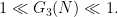
From Mertens’ theorem we see that

\displaystyle  \prod_p E_p(\frac{1+it_1}{\log R},\frac{1+it_2}{\log R},\frac{1+it_3}{\log R}) \ll \prod_p (1 + O(\frac{1}{p^{1+1/\log R}}) )

\displaystyle  \ll \log^{O(1)} R

so from the rapid decrease of {F} we may restrict {t_1,t_2,t_3} to be bounded in magnitude by {\sqrt{\log R}} accepting a negligible error of {O_A(\log^{-A} R)}. Using

\displaystyle  \prod_p 1 - \frac{1}{p^s} = \frac{1}{\zeta(s)}

for {\hbox{Re}(s)=1}, we can write

\displaystyle  \prod_p E_p(s_1,s_2,s_3) = \frac{1}{\zeta(1+s_1) \zeta(1+s_2) \zeta(1+s_3)}

\displaystyle  \prod_p E_p(s_1,s_2,s_3) \prod_{j=1}^3 (1 - \frac{1}{p^{1+s_j}})^{-1}.

By Taylor expansion, we have
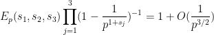
\displaystyle  E_p(s_1,s_2,s_3) \prod_{j=1}^3 (1 - \frac{1}{p^{1+s_j}})^{-1} = 1 + O( \frac{1}{p^{3/2}} )

(say) uniformly for {|s_1|, |s_2|, |s_3| \leq 1/10}, and so the logarithm of the product {\prod_p E_p(s_1,s_2,s_3) \prod_{j=1}^3 (1 - \frac{1}{p^{1+s_j}})^{-1}} is a bounded holomorphic function in this region. From Taylor expansion we thus have

\displaystyle  \prod_p E_p(s_1,s_2,s_3) \prod_{j=1}^3 (1 - \frac{1}{p^{1+s_j}})^{-1} = (1+P(s_1,s_2,s_3)+O_A(\log^{-A} R))

\displaystyle  \times \prod_p E_p(0,0,0) / (1 - \frac{1}{p})^3

when {s_1,s_2,s_3 = O( 1/\sqrt{\log R} )}, where {P} is some polynomial (depending on {A}) with vanishing constant term. From (1) we see that

\displaystyle  \prod_p E_p(0,0,0) / (1 - \frac{1}{p})^3 = G_3(N).

Similarly we have

\displaystyle  \zeta(1+s) = \frac{1 + Q(s) + O_A( \log^{-A} R)}{s}

for {s = O(1/\sqrt{\log R})}, where {Q} is another polynomial depending on {A} with vanishing constant term. We can thus write (26) (up to errors of {O_A(\log^{-A} R)}) as

\displaystyle  G_3(N) \int_{|t_1|, |t_2|, |t_3| \leq \sqrt{\log R}} (1+S(\frac{1+it_1}{\log R},\frac{1+it_2}{\log R},\frac{1+it_3}{\log R}))

\displaystyle  (1+it_1) (1+it_2) (1+it_3) F(t_1) F(t_2) F(t_3)\ dt_1 dt_2 dt_3

where {S} is a polynomial depending on {A} with vanishing constant term. By the rapid decrease of {F} we may then remove the constraints on {t_1,t_2,t_3}, and reduce (24) to showing that

\displaystyle  \int_{\bf R} \int_{\bf R} \int_{\bf R} (1+S(\frac{1+it_1}{\log R},\frac{1+it_2}{\log R},\frac{1+it_3}{\log R}))

\displaystyle  (1+it_1) (1+it_2) (1+it_3) F(t_1) F(t_2) F(t_3)\ dt_1 dt_2 dt_3 = 1

which on expanding {S} and Fubini’s theorem reduces to showing that

\displaystyle  \int_{\bf R} (1+it)^k F(t)\ dt = 1_{k=1}

for {k=1,2,\dots}. But from multiplying (25) by {e^{-u}} and then differentiating {k} times at {u=0}, we see that

\displaystyle  \eta^{(k)}(0) = (-1)^k \int_{\bf R} (1+it)^k F(t)\ dt,

and the claim follows since {\eta(u) = 1-u} for {0 \leq u \leq 1/2}. This proves Theorem 2 and hence Theorem 1.
One can of course use other approximations to {\Lambda} to establish Vinogradov’s theorem. The following exercise gives one such route:

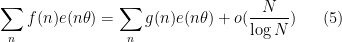
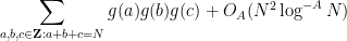
Exercise 31 Use Exercise 27 to obtain the asymptotic

\displaystyle  \sum_{a,b,c: a+b+c=N} \Lambda(a) \Lambda(b) \Lambda(c)

\displaystyle = \frac{N^2}{2} \sum_{q \leq Q} \sum_{a \in ({\bf Z}/q{\bf Z})^\times} \frac{\mu(q)}{\phi(q)^3} e( aN/q) + O_A( N^2 \log^{-A} N )

for any {A>0} with ineffective constants. Then show that

\displaystyle  \sum_q \sum_{a \in ({\bf Z}/q{\bf Z})^\times} \frac{\mu(q)}{\phi(q)^3} e( aN/q) = G_3(N)

and give an alternate derivation of Theorem 2.

Exercise 32 By using Exercise 26 in place of Exercise 27, obtain the asymptotic

\displaystyle  \sum_{a,b,c: a+b+c=N} \Lambda(a) \Lambda(b) \Lambda(c)

\displaystyle = (G_3(N) + O( \frac{q^2}{\phi(q)^3}) ) \frac{N^2}{2} + O_A( N^2 \log^{-A} N )

for any {A>0} with effective constants if there is a real primitive Dirichlet character {\chi} of modulus {q} and modulus {q \leq \log^B x} and an exceptional {\beta} with {1 - \frac{c}{\log q} \leq \beta < 1} for some sufficiently small {c} and for some sufficiently large {B} depending on {A}, with the {\chi(N) \frac{\tau(\chi)^4}{\phi(q)^3}} term being deleted if no such exceptional character exists. Use this to establish Theorem 1 with an effective bound on how sufficiently large {N} has to be.

Exercise 33 Let {N \geq 2}. Show that

\displaystyle  \sum_{a,r: a+2r \leq N} \Lambda(a) \Lambda(a+r) \Lambda(a+2r) = {\mathfrak S} \frac{N^2}{4} + O_A( N^2 \log^{-A} N )

for any {A > 0}, where

\displaystyle  {\mathfrak S} := \frac{3}{2} \prod_{p>3} (1-\frac{2}{p}) (1-\frac{1}{p})^{-2}.

Conclude that the number of length three arithmetic progressions {a,a+r,a+2r} contained in the primes up to {N} is {{\mathfrak S} \frac{N^2}{4\log^3 N} + O_A( N^2 \log^{-A} N )} for any {A > 0}. (This result is due to van der Corput.)

Exercise 34 (Even Goldbach conjecture for most {N}) Let {N \geq 2}, and let {g} be as in (23).

  • (i) Show that {\Lambda(f,f,h) = \Lambda(g,g,h) + O_A( N^2 \log^{-A} N )} for any {A > 0} and any function {h: \{1,\dots,N\} \rightarrow {\bf R}} bounded in magnitude by {1}.
  • (ii) For any {M \leq N}, show that

    \displaystyle  \sum_{a,b: a+b=M} g(a) g(b) = G_2(M) M + O_A( N \log^{-A} N )

    for any {A > 0}, where

    \displaystyle  G_2(M) := \prod_{p|M} \frac{p^2-p}{(p-1)^2} \times \prod_{p \not | M} \frac{p^2-2p}{(p-1)^2}.

  • (iii) Show that for any {A > 0}, one has

    \displaystyle  \sum_{a,b: a+b=M} f(a) f(b) = G_2(M) M + O_A( N \log^{-A} N )

    for all but at most {O_A( N \log^{-A} N )} of the numbers {M \in \{1,\dots,N\}}.

  • (iv) Show that all but at most {O_A( N \log^{-A} N )} of the even numbers in {\{1,\dots,N\}} are expressible as the sum of two primes.