An improved Type I estimate

27 July, 2013 in math.NT, polymath | Tags: Deligne's theorem, dispersion method, exponential sums, polymath8, Type I estimate

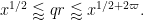
As in all previous posts in this series, we adopt the following asymptotic notation: ${x}$ is a parameter going off to infinity, and all quantities may depend on ${x}$ unless explicitly declared to be “fixed”. The asymptotic notation ${O(), o(), \ll}$ is then defined relative to this parameter. A quantity ${q}$ is said to be of polynomial size if one has ${q = O(x^{O(1)})}$ , and bounded if ${q=O(1)}$ . We also write ${X \lessapprox Y}$ for ${X \ll x^{o(1)} Y}$ , and ${X \sim Y}$ for ${X \ll Y \ll X}$ .

The purpose of this (rather technical) post is both to roll over the polymath8 research thread from this previous post, and also to record the details of the latest improvement to the Type I estimates (based on exploiting additional averaging and using Deligne’s proof of the Weil conjectures) which lead to a slight improvement in the numerology.

In order to obtain this new Type I estimate, we need to strengthen the previously used properties of “dense divisibility” or “double dense divisibility” as follows.

Definition 1 (Multiple dense divisibility) Let ${y \geq 1}$ . For each natural number ${k \geq 0}$ , we define a notion of ${k}$ -tuply ${y}$ -dense divisibility recursively as follows:

Every natural number ${n}$ is ${0}$ -tuply ${y}$ -densely divisible.

If ${k \geq 1}$ and ${n}$ is a natural number, we say that ${n}$ is ${k}$ -tuply ${y}$ -densely divisible if, whenever ${i,j \geq 0}$ are natural numbers with ${i+j=k-1}$ , and ${1 \leq R \leq n}$ , one can find a factorisation ${n = qr}$ with ${y^{-1} R \leq r \leq R}$ such that ${q}$ is ${i}$ -tuply ${y}$ -densely divisible and ${r}$ is ${j}$ -tuply ${y}$ -densely divisible.

We let ${{\mathcal D}^{(k)}_y}$ denote the set of ${k}$ -tuply ${y}$ -densely divisible numbers. We abbreviate “ ${1}$ -tuply densely divisible” as “densely divisible”, “ ${2}$ -tuply densely divisible” as “doubly densely divisible”, and so forth; we also abbreviate ${{\mathcal D}^{(1)}_y}$ as ${{\mathcal D}_y}$ .

Given any finitely supported sequence ${\alpha: {\bf N} \rightarrow {\bf C}}$ and any primitive residue class ${a\ (q)}$ , we define the discrepancy

$\displaystyle \Delta(\alpha; a \ (q)) := \sum_{n: n = a\ (q)} \alpha(n) - \frac{1}{\phi(q)} \sum_{n: (n,q)=1} \alpha(n).$

We now recall the key concept of a coefficient sequence, with some slight tweaks in the definitions that are technically convenient for this post.

Definition 2 A coefficient sequence is a finitely supported sequence ${\alpha: {\bf N} \rightarrow {\bf R}}$ that obeys the bounds

$\displaystyle |\alpha(n)| \ll \tau^{O(1)}(n) \log^{O(1)}(x) \ \ \ \ \ (1)$

for all ${n}$ , where ${\tau}$ is the divisor function.

(i) A coefficient sequence ${\alpha}$ is said to be located at scale ${N}$ for some ${N \geq 1}$ if it is supported on an interval of the form ${[cN, CN]}$ for some ${1 \ll c < C \ll 1}$ .

(ii) A coefficient sequence ${\alpha}$ located at scale ${N}$ for some ${N \geq 1}$ is said to obey the Siegel-Walfisz theorem if one has
$\displaystyle | \Delta(\alpha 1_{(\cdot,q)=1}; a\ (r)) | \ll \tau(qr)^{O(1)} N \log^{-A} x \ \ \ \ \ (2)$

for any ${q,r \geq 1}$ , any fixed ${A}$ , and any primitive residue class ${a\ (r)}$ .

(iii) A coefficient sequence ${\alpha}$ is said to be smooth at scale ${N}$ for some ${N > 0}$ is said to be smooth if it takes the form ${\alpha(n) = \psi(n/N)}$ for some smooth function ${\psi: {\bf R} \rightarrow {\bf C}}$ supported on an interval of size ${O(1)}$ and obeying the derivative bounds
$\displaystyle |\psi^{(j)}(t)| \lesssim \log^{O(1)} x \ \ \ \ \ (3)$

for all fixed ${j \geq 0}$ (note that the implied constant in the ${O()}$ notation may depend on ${j}$ ).

Note that we allow sequences to be smooth at scale ${N}$ without being located at scale ${N}$ ; for instance if one arbitrarily translates of a sequence that is both smooth and located at scale ${N}$ , it will remain smooth at this scale but may not necessarily be located at this scale any more. Note also that we allow the smoothness scale ${N}$ of a coefficient sequence to be less than one. This is to allow for the following convenient rescaling property: if ${n \mapsto \psi(n)}$ is smooth at scale ${N}$ , ${q \geq 1}$ , and ${a}$ is an integer, then ${n \mapsto \psi(qn+a)}$ is smooth at scale ${N/q}$ , even if ${N/q}$ is less than one.

Now we adapt the Type I estimate to the ${k}$ -tuply densely divisible setting.

Definition 3 (Type I estimates) Let ${0 < \varpi < 1/4}$ , ${0 < \delta < 1/4+\varpi}$ , and ${0 < \sigma < 1/2}$ be fixed quantities, and let ${k \geq 1}$ be a fixed natural number. We let ${I}$ be an arbitrary bounded subset of ${{\bf R}}$ , let ${P_I := \prod_{p \in I} p}$ , and let ${a\ (P_I)}$ a primitive congruence class. We say that ${Type^{(k)}_I[\varpi,\delta,\sigma]}$ holds if, whenever ${M, N \gg 1}$ are quantities with

$\displaystyle M N \sim x \ \ \ \ \ (4)$

and

$\displaystyle x^{1/2-\sigma} \lessapprox N \lessapprox x^{1/2-2\varpi-c} \ \ \ \ \ (5)$

for some fixed ${c>0}$ , and ${\alpha,\beta}$ are coefficient sequences located at scales ${M,N}$ respectively, with ${\beta}$ obeying a Siegel-Walfisz theorem, we have

$\displaystyle \sum_{q \in {\mathcal S}_I \cap {\mathcal D}_{x^\delta}^{(k)}: q \leq x^{1/2+2\varpi}} |\Delta(\alpha * \beta; a\ (q))| \ll x \log^{-A} x \ \ \ \ \ (6)$

for any fixed ${A>0}$ . Here, as in previous posts, ${{\mathcal S}_I}$ denotes the square-free natural numbers whose prime factors lie in ${I}$ .

The main theorem of this post is then

Theorem 4 (Improved Type I estimate) We have ${Type^{(4)}_I[\varpi,\delta,\sigma]}$ whenever

$\displaystyle \frac{160}{3} \varpi + 16 \delta + \frac{34}{9} \sigma < 1$

and

$\displaystyle 64\varpi + 18\delta + 2\sigma < 1.$

In practice, the first condition here is dominant. Except for weakening double dense divisibility to quadruple dense divisibility, this improves upon the previous Type I estimate that established ${Type^{(2)}_I[\varpi,\delta,\sigma]}$ under the stricter hypothesis

$\displaystyle 56 \varpi + 16 \delta + 4 \sigma < 1.$

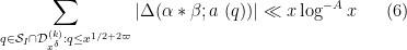
As in previous posts, Type I estimates (when combined with existing Type II and Type III estimates) lead to distribution results of Motohashi-Pintz-Zhang type. For any fixed ${\varpi, \delta > 0}$ and ${k \geq 1}$ , we let ${MPZ^{(k)}[\varpi,\delta]}$ denote the assertion that

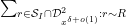
$\displaystyle \sum_{q \in {\mathcal S}_I \cap {\mathcal D}_{x^\delta}^{(k)}: q \leq x^{1/2+2\varpi}} |\Delta(\Lambda 1_{[x,2x]}; a\ (q))| \ll x \log^{-A} x \ \ \ \ \ (7)$

for any fixed ${A > 0}$ , any bounded ${I}$ , and any primitive ${a\ (P_I)}$ , where ${\Lambda}$ is the von Mangoldt function.

Corollary 5 We have ${MPZ^{(4)}[\varpi,\delta]}$ whenever

$\displaystyle \frac{600}{7} \varpi + \frac{180}{7} \delta < 1 \ \ \ \ \ (8)$

Proof: Setting ${\sigma}$ sufficiently close to ${1/10}$ , we see from the above theorem that ${Type^{(4)}_{II}[\varpi,\delta]}$ holds whenever

$\displaystyle \frac{600}{7} \varpi + \frac{180}{7} \delta < 1$

and

$\displaystyle 80 \varpi + \frac{45}{2} \delta < 1.$

The second condition is implied by the first and can be deleted.

From this previous post we know that ${Type^{(4)}_{II}[\varpi,\delta]}$ (which we define analogously to ${Type'_{II}[\varpi,\delta], Type''_{II}[\varpi,\delta]}$ from previous sections) holds whenever

$\displaystyle 68 \varpi + 14 \delta < 1$

while ${Type^{(4)}_{III}[\varpi,\delta,\sigma]}$ holds with ${\sigma}$ sufficiently close to ${1/10}$ whenever

$\displaystyle 70 \varpi + 5 \delta < 1.$

Again, these conditions are implied by (8). The claim then follows from the Heath-Brown identity and dyadic decomposition as in this previous post. $\Box$

As before, we let ${DHL[k_0,2]}$ denote the claim that given any admissible ${k_0}$ -tuple ${{\mathcal H}}$ , there are infinitely many translates of ${{\mathcal H}}$ that contain at least two primes.

Corollary 6 We have ${DHL[k_0,2]}$ with ${k_0 = 632}$ .

This follows from the Pintz sieve, as discussed below the fold. Combining this with the best known prime tuples, we obtain that there are infinitely many prime gaps of size at most ${4,680}$ , improving slightly over the previous record of ${5,414}$ .

— 1. Multiple dense divisibility —

We record some useful properties of dense divisibility.

Lemma 7 (Properties of dense divisibility) Let ${k \geq 0}$ and ${y \geq 1}$ .

(i) If ${n}$ is ${k}$ -tuply ${y}$ -densely divisible, and ${m}$ is a factor of ${n}$ , then ${m}$ is ${k}$ -tuply ${y (n/m)}$ -densely divisible. Similarly, if ${l}$ is a multiple of ${n}$ , then ${l}$ is ${y (l/n)}$ -densely divisible.

(ii) If ${m,n}$ are ${y}$ -densely divisible, then ${[m,n]}$ is also ${y}$ -densely divisible.

(iii) Any ${y}$ -smooth number is ${k}$ -tuply ${y}$ -densely divisible.

(iv) If ${n}$ is ${y'}$ -smooth and square-free for some ${y' \geq y}$ , and ${\prod_{p|n: p \leq y} p \geq (y')^k/y}$ , then ${n}$ is ${k}$ -tuply ${y}$ -densely divisible.

Proof: (i) is easily established by induction on ${k}$ , the idea being to start with a good factorisation of ${n}$ and perturb it into a factorisation of ${m}$ or ${l}$ by dividing or multiplying by a small number. To prove (ii), we may assume without loss of generality that ${m \leq n}$ , so that ${n \geq [m,n]^{1/2}}$ . If we set ${a := \frac{[m,n]}{n}}$ , then the factors of ${n}$ , as well as the factors of ${n}$ multiplied by ${a}$ , are both factors of ${[m,n]}$ . From this we can deduce the ${y}$ -dense divisibility of ${[m,n]}$ from the ${y}$ -dense divisibility of ${n}$ .

The claim (iii) is easily established by induction on ${k}$ and a greedy algorithm, so we turn to (iv). The claim is trivial for ${k=0}$ . Next, we consider the ${k=1}$ case. Our task is to show that for any ${1 \leq R \leq n}$ , one can find a factorisation ${n=qr}$ with ${y^{-1} R \leq r \leq R}$ . If ${\prod_{p|n: p>y} p \leq R}$ , we can achieve this factorisation by initialising ${r}$ to equal ${\prod_{p|n: p>y} p}$ and then greedily multiplying the remaining factors of ${n}$ until one exceeds ${y^{-1} R}$ , so we may assume instead that ${\prod_{p|n: p>y} p > R}$ . Then by the greedy algorithm we can find a factor ${r'}$ of ${\prod_{p|n: p>y} p}$ with ${(y')^{-1} R \leq r' \leq R}$ ; if we then greedily multiply ${r'}$ by factors ${p|n}$ with ${p<y}$ we obtain the claim.

Finally we consider the ${k>1}$ case. We assume inductively that the claim has already been proven for smaller values of ${k}$ . Let ${i,j \geq 0}$ be such that ${i+j=k-1}$ . By hypothesis, the ${y}$ -smooth quantity ${n' := \prod_{p|n: p \geq y} p}$ is at least ${(y')^i (y')^j (y'/y)}$ . By the greedy algorithm, we may thus factor ${n' = n_1 n_2 n_3}$ where

$\displaystyle (y')^i y^{-1} \leq n_1 \leq (y')^i$

and

$\displaystyle (y')^j y^{-1} \leq n_2 \leq (y')^j$

and thus

$\displaystyle n_3 \geq y'/y.$

Now we divide into several cases. Suppose first that ${n_1 \leq R \leq n/n_2}$ . Then ${1 \leq \frac{R}{n_1} \leq \frac{n}{n_1 n_2}}$ , so by the ${k=1}$ case, we may find a factorisation ${\frac{n}{n_1 n_2} = q' r'}$ with ${y^{-1} \frac{R}{n_1} \leq r' \leq \frac{R}{n_1}}$ . Setting ${r := n_1 r'}$ and ${q := n_2 q'}$ , the claim then follows from the induction hypothesis.

Now suppose that ${R < n_1}$ . By the greedy algorithm, we may then find a factor ${r}$ of the ${y}$ -smooth quantity ${n_1}$ with ${y^{-1} R \leq r \leq R}$ ; setting ${q := n/r}$ , we see that ${q}$ is a multiple of ${n_2}$ and hence ${\prod_{p|q: p \leq y} p \geq (y')^j y^{-1}}$ . The claim now follows from the induction hypothesis and (iii).

Finally, suppose that ${R > n/n_2}$ . By the greedy algorithm, we may then find a factor ${q}$ of the ${y}$ -smooth quantity ${n_2}$ with ${n/R \leq q \leq yn/R}$ ; setting ${r := n/q}$ , we see that ${r}$ is a multiple of ${n_1}$ and hence ${\prod_{p|r: p \leq y} p \geq (y')^i y^{-1}}$ . The claim now follows from the induction hypothesis and (iii). $\Box$

Now we record the criterion for using ${MPZ^{(k)}}$ to deduce ${DHL[k_0,2]}$ .

Proposition 8 (Criterion for DHL) Let ${\varpi, \delta}$ be such that ${MPZ^{(k)}[\varpi,\delta]}$ holds. Suppose that one can find a natural number ${k_0 > 2}$ and real numbers ${\delta \leq \delta' \leq 1/4+\varpi}$ and ${A > 0}$ such that

$\displaystyle (1+4\varpi) (1-2\kappa_1 - 2\kappa_2 - 2\kappa_3) > \frac{j^{2}_{k_0-2}}{k_0(k_0-1)}$

where

$\displaystyle \kappa_1 := \int_{\theta}^1 (1-t)^{(k_0-1)/2} \frac{dt}{t}$

$\displaystyle \kappa_2 := (k_0-1) \int_{\theta}^1 (1-t)^{k_0-1} \frac{dt}{t}$

$\displaystyle \kappa_3 := \tilde \theta \frac{J_{k_0-2}(\sqrt{\tilde \theta} j_{k_0-2})^2 - J_{k_0-3}(\sqrt{\tilde \theta} j_{k_0-2}) J_{k_0-1}(\sqrt{\tilde \theta} j_{k_0-2})}{ J_{k_0-3}(j_{k_0-2})^2 }$

$\displaystyle \times \exp( A + (k_0-1) \int_{\tilde \delta}^\theta e^{-(A+2\alpha)t} \frac{dt}{t} )$

$\displaystyle \alpha := \frac{j_{k_0-2}^2}{4(k_0-1)}$

$\displaystyle \theta := \frac{\delta'}{1/4 + \varpi}$

$\displaystyle \tilde \theta := \frac{k\delta' - \delta/2 + \varpi}{1/4 + \varpi}$

$\displaystyle \tilde \delta := \frac{\delta}{1/4 + \varpi}.$

Then ${DHL[k_0,2]}$ holds.

Proof: We use the Pintz sieve from this post, repeating the proof of Theorem 5 from that post (and using the explicit formulae for ${G_{k_0-1}(0,0)}$ and ${G_{k_0-1,\tilde \theta}(0,0)}$ from this comment thread). The main difference is that the exponent ${(\delta'-\delta)/2 + \varpi + \epsilon/2}$ in equation (10) of that post needs to be replaced with ${(k\delta'-\delta)/2 + \varpi + \epsilon/2}$ (and similarly for the displays up to (11)), and ${{\mathcal D}_{x^\delta}}$ needs to be replaced with ${{\mathcal D}_{x^\delta}^{(k)}}$ . $\Box$

Applying this proposition with ${k_0 := 632}$ , ${\delta = 1/11500}$ , ${\delta' := 1/128}$ , ${600 \varpi/7 + 180 \delta / 7}$ sufficiently close to ${1}$ , and ${A := 200}$ we obtain ${DHL[632,2]}$ as claimed.

— 2. van der Corput estimates —

In this section we generalise the van der Corput estimates from Section 1 of this previous post to wider classes of “structured functions” than rational phases. We will adopt an axiomatic approach, laying out the precise axioms that we need a given class of structured functions to obey:

Definition 9 (Structured functions) Let ${I}$ be a bounded subset of ${{\bf R}}$ . A class of structured functions is a family ${{\mathcal C} = ({\mathcal C}_{p,C})_{p,C}}$ of collections ${{\mathcal C}_{p,C}}$ of functions ${K:U \rightarrow {\bf C}}$ defined on subsets ${U}$ of ${{\bf Z}/p{\bf Z}}$ for each prime ${p \in I}$ and every ${C \geq 1}$ ; an element of ${{\mathcal C}_{p,C}}$ is then said to be a structured function of complexity at most ${C}$ and modulus ${p}$ . Furthermore we place an equivalence relation ${\equiv}$ on each class ${{\mathcal C}_{p,C}}$ with ${p}$ sufficiently large depending on ${C}$ . This class and this equivalence relation is assumed to obey the following axioms:

(i) (Monotonicity) One has ${{\mathcal C}_{p,C} \subset {\mathcal C}_{p,C'}}$ whenever ${C' \geq C}$ . Furthermore, if ${p}$ is sufficiently large depending on ${C,C'}$ , the equivalence relations on ${{\mathcal C}_{p,C}}$ and ${{\mathcal C}_{p,C'}}$ agree on their common domain of definition.

(ii) (Near-total definition) If ${K \in {\mathcal C}_{p,C}}$ , then the domain ${U}$ of ${K}$ consists of ${{\bf Z}/p{\bf Z}}$ with at most ${O_C(1)}$ points removed.

(iii) (Pointwise bound) If ${K \in {\mathcal C}_{p,C}}$ , then ${K(x) = O_C(1)}$ for all ${x}$ in the domain ${U}$ of ${K}$ .

(iv) (Conjugacy) If ${K \in {\mathcal C}_{p,C}}$ , then ${\overline{K} \in {\mathcal C}_{p,C'}}$ for some ${C' = O_C(1)}$ .

(v) (Multiplication) If ${K,K' \in {\mathcal C}_{p,C}}$ , then the pointwise product ${KK'}$ (on the common domain of definition) can be expressed as the sum of ${k=O_C(1)}$ functions ${K_1,\ldots,K_k}$ (which we will call the components of ${KK'}$ ) in ${{\mathcal C}_{p,C'}}$ for some ${C' = O_C(1)}$ .

(vi) (Translation invariance) If ${K \in {\mathcal C}_{p,C}}$ , and ${h \in {\bf Z}/p{\bf Z}}$ , then the function ${x \mapsto K(x+h)}$ (defined on the translation ${U-h}$ of the domain of definition of ${K}$ ) lies in ${{\mathcal C}_{p,C'}}$ for some ${C' = O_C(1)}$ .

(vii) (Dilation invariance) If ${K \in {\mathcal C}_{p,C}}$ , and ${a \in ({\bf Z}/p{\bf Z})^\times}$ , then the function ${x \mapsto K(ax)}$ (defined on the dilation ${a^{-1} U}$ of the domain of definition of ${f}$ ) lies in ${{\mathcal C}_{p,C'}}$ for some ${C' = O_C(1)}$ .

(viii) (Polynomial phases) If ${P: {\bf Z}/p{\bf Z} \rightarrow {\bf Z}/p{\bf Z}}$ is a polynomial of degree at most ${d}$ , then the function ${x \mapsto e_p(P(x))}$ lies in ${{\mathcal C}_{p,C}}$ for some ${C = O_d(1)}$ . More generally, if ${K \in {\mathcal C}_{p,C}}$ , then the product ${x \mapsto e_p(P(x)) K(x)}$ lies in ${{\mathcal C}_{p,C'}}$ for some ${C' = O_{C,d}(1)}$ . Furthermore, if ${p}$ is sufficiently large depending on ${d,C}$ , this operation respects the equivalence relation ${\equiv}$ : ${K \equiv K'}$ if and only if ${e_p(P) K \equiv e_p(P) K'}$ . Finally, if ${K \equiv e_p(P)}$ and ${K}$ is not identically zero, then ${c_{K,e_p(P)} \neq 0}$ .

(ix) (Almost orthogonality) If ${K,K' \in {\mathcal C}_{p,C}}$ have domains of definition ${U, U'}$ respectively, one has ${\sum_{x \in U \cap U'} K(x) \overline{K'(x)} = c_{K,K'} p + O_C(p^{1/2})}$ for an algebraic integer ${c_{K,K'}}$ , with the error term ${O_C(p^{1/2})}$ being Galois-absolute in the sense that all Galois conjugates of the error term are also ${O_C(p^{1/2})}$ . Furthermore, if ${p}$ is sufficiently large depending on ${C}$ , then ${c_{K,K'}}$ vanishes whenever ${K \not \equiv K'}$ .

(x) (Integration) Suppose that ${K \in {\mathcal C}_{p,C}}$ is such that ${K(\cdot+h) \overline{K}}$ contains a component equivalent to ${1}$ for some ${h \in ({\bf Z}/p{\bf Z})^\times}$ . Suppose also that ${p}$ is sufficiently large depending on ${C}$ . Then there exists ${a \in {\bf Z}/p{\bf Z}}$ such that ${K \equiv e_p(a \cdot)}$ .

Example 1 (Polynomial phases) Let ${I}$ be a bounded subset of ${{\bf R}}$ . If, for every prime ${p \in I}$ and ${C \geq 1}$ , we define ${{\mathcal C}_{p,C}}$ to be the set of all functions of the form ${x \mapsto e_p(f(x))}$ , where ${f}$ are polynomials of degree at most ${C}$ with integer coefficients, defined on all of ${{\bf Z}/p{\bf Z}}$ , then this is a class of structured functions (note that the almost orthogonality axiom requires the Weil conjectures for curves). Two polyomial phases ${e_p(f(x)), e_p(g(x))}$ will be declared equivalent if ${f,g}$ differ only in the constant term. Note from the Chinese remainder theorem that the function ${x \mapsto e_q( f(x) )}$ is then also a structured function of complexity at most ${C}$ and modulus ${q}$ .

Example 2 (Polynomial phases twisted by characters) Let ${I}$ be a bounded subset of ${{\bf R}}$ . If, for every prime ${p \in I}$ and ${C \geq 1}$ , we define ${{\mathcal C}_{p,C}}$ to be the set of all functions of the form ${x \mapsto e(\theta) e_p(f(x)) \prod_{i=1}^k \chi_i( g_i(x) )}$ , where ${e(\theta)}$ is a phase, ${g_i,f}$ are polynomials of degree at most ${C}$ with integer coefficients, ${0 \leq k \leq C}$ , and the ${\chi_i}$ are Dirichlet characters of order ${p}$ , with the non-standard convention that ${\chi_i}$ is undefined (instead of vanishing) at zero. Then this is a class of structured functions (again, the almost orthogonality axiom requires the Weil conjectures for curves). We declare two structured functions to be equivalent if they agree up to a constant phase on their common domain of definition. Note from the Chinese remainder theorem that the function ${x \mapsto e_q( f(x) ) \prod_{i=1}^k \chi_i(g_i(x))}$ is then also a structured function of complexity at most ${C}$ if the ${\chi_i}$ are Dirichlet characters of period ${q}$ (and conductor dividing ${q}$ ), again with the convention that ${\chi(x)}$ is undefined (instead of vanishing) when ${(x,q) \neq 1}$ .

Example 3 (Rational phases) Let ${I}$ be a bounded subset of ${{\bf R}}$ . If, for every prime ${p \in I}$ and ${C \geq 1}$ , we define ${{\mathcal C}_{p,C}}$ to be the set of all functions of the form ${x \mapsto e_p(\frac{f(x)}{g(x)})}$ , where ${f,g}$ are polynomials of degree at most ${C}$ with integer coefficients and with ${g}$ monic, with the function only defined when ${g(x) \neq 0}$ , then this is a class of structured functions (again, the almost orthogonality axiom requires the Weil conjectures for curves). We declare two structured functions to be equivalent if they agree up to a constant phase on their common domain of definition. Note from the Chinese remainder theorem that the function ${x \mapsto e_q( \frac{f(x)}{g(x)})}$ is then also a structured function of complexity at most ${C}$ and modulus ${q}$ .

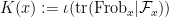
Example 4 (Trace weights) Let ${I}$ be a bounded subset of ${{\bf R}}$ . We fix a prime ${\ell}$ not in ${I}$ , and we fix an embedding ${\iota: {\bf Q}_\ell \rightarrow {\bf C}}$ of the ${\ell}$ -adics into ${{\bf C}}$ . If, for every prime ${p \in I}$ and ${C \geq 1}$ , we define ${{\mathcal C}_{p,C}}$ to be the set of all functions ${K = K_{\mathcal F}: U \rightarrow {\bf C}}$ of the form

$\displaystyle K(x) := \iota( \hbox{tr}( \hbox{Frob}_x | {\mathcal F}_x ) )$

where ${U}$ is ${{\Bbb F}_p = {\bf Z}/p{\bf Z}}$ with at most ${C}$ points removed, and ${{\mathcal F}}$ is a lisse ${\ell}$ -adic sheaf on ${U}$ that is pure of weight ${0}$ and geometrically isotypic with conductor at most ${C}$ (see this previous post for definitions of these terms), then this is a class of structured functions. We declare two trace weights ${K, K'}$ to be equivalent if one has ${K = K_{\mathcal F}}$ and ${K' = K_{{\mathcal F}'}}$ for some geometrically isotypic sheaves ${{\mathcal F}, {\mathcal F}'}$ whose geometrically irreducible components are isomorphic. The almost orthogonality now is deeper, being a consequence of Deligne’s second proof of the Weil conjectures, and also using a form of Schur’s lemma for sheaves; see Section 5 of this paper of Fouvry, Kowalski, and Michel. The integration axiom follows from Lemma 5.3 of the same paper. This class of structured functions includes the previous three classes, but also includes Kloosterman-type objects such as ${x \mapsto \frac{1}{\sqrt{p}} \sum_{y \in {\Bbb F}_p^\times} e_p( \frac{1}{y} + xy)}$ (and many other exponential sums) besides. (Indeed, it basically closed under the operations of Fourier transforms, convolution, and pullback, as long as certain degenerate cases are avoided.)

We now turn to the problem of obtaining non-trivial bounds for the expression

$\displaystyle \sum_n \psi_N(n) K_q(n)$

where ${q \in {\mathcal S}_I}$ , ${K_q}$ is a structured function of bounded complexity and modulus ${q}$ , and ${\psi_N}$ is a smooth function at scale ${N}$ . The trivial bound here is

$\displaystyle \sum_n \psi_N(n) K_q(n)| \lessapprox N,$

since one has ${|K_q(n)| \lessapprox 1}$ from the divisor bound. In some cases we cannot hope to improve upon this bound; for instance, if ${K_q}$ is a constant phase ${e(\theta)}$ then there is clearly no improvement available. Similarly, if ${K_q}$ is the linear phase ${K_q(n) = e_q(n) e(\theta)}$ , then there is no improvement in the regime ${N \ll q}$ ; if ${K_q}$ is the quadratic phase ${K_q(n) = e_q(n^2) e(\theta)}$ then there is no improvement in the regime ${N \ll q^{1/2}}$ ; if ${K_q}$ is the cubic phase ${K_q(n) = e_q(n^3) e(\theta)}$ then there is no improvement in the regime ${N \ll q^{1/3}}$ ; and so forth. On the other hand, we will be able to establish a van der Corput estimate which roughly speaking asserts that as long as these polynomial obstructions are avoided, and ${q}$ is smooth, one gets a non-trivial gain.

We first need a lemma:

Lemma 10 (Fundamental theorem of calculus) Let ${{\mathcal C}}$ be a class of structured functions. Let ${C, d \geq 0}$ , let ${p \in I}$ , and let ${K}$ be a structured function of complexity at most ${C}$ with modulus ${p}$ . Assume that ${p}$ is sufficiently large depending on ${C,d}$ . Let ${h \in ({\bf Z}/p{\bf Z})^\times}$ , and suppose that there is a polynomial ${P: {\bf Z}/p{\bf Z} \rightarrow {\bf Z}/p{\bf Z}}$ of degree at most ${d}$ such that ${K(\cdot+h) \overline{K} \equiv e_p(P)}$ for all ${n \in {\bf Z}/p{\bf Z}}$ for which this identity is well-defined. Then there exists a polynomial ${Q: {\bf Z}/p{\bf Z} \rightarrow {\bf Z}/p{\bf Z}}$ of degree at most ${d+1}$ such that ${K \equiv e_p(Q)}$ for all ${n \in {\bf Z}/p{\bf Z}}$ for which this identity is well-defined.

Proof: By dilating by ${h}$ and using the dilation invariance of structured functions, we may assume without loss of generality that ${h=1}$ . We can write ${P}$ in terms of the binomial functions ${n \mapsto \binom{n}{i}}$ for ${i=0,\ldots,d}$ (which are well-defined if ${p > d}$ ) as

$\displaystyle P(n) = \sum_{i=0}^d c_i \binom{n}{i}$

for some coefficients ${c_0,\ldots,c_d\in {\bf Z}/p{\bf Z}}$ . If we then define

$\displaystyle Q_0(n) := \sum_{i=0}^d c_i \binom{n}{i+1}$

then ${Q_0}$ is a polynomial of degree at most ${d+1}$ (if ${p>d+1}$ ) and ${Q_0(n+1)-Q_0(n)=P(n)}$ by Pascal’s identity. So if we multiply ${K}$ by ${e_p(-Q_0)}$ (using the polynomial phase invariance of structured functions) we may assume without loss of generality that ${P=0}$ , thus ${K(\cdot+1) \overline{K} \equiv 1}$ . But then the claim follows from the integration axiom. $\Box$

Now we can state the van der Corput estimate.

Proposition 11 (van der Corput) Let ${{\mathcal C}}$ be a class of structured functions. Let ${q \in {\mathcal S}_I}$ be of polynomial size, and let ${K_q = \prod_{p|q} K_p}$ be a structured function of modulus ${q}$ and complexity at most ${O(1)}$ . Let ${l \geq 1}$ be fixed, and let ${{\mathcal P}}$ denote the set of sufficiently large primes ${p}$ dividing ${q}$ with the property that there exists a polynomial ${P_p: {\bf Z}/p{\bf Z} \rightarrow {\bf Z}/p{\bf Z}}$ of degree at most ${l}$ such that ${c_{K_p,e_p(P_p)} \neq 0}$ , and let ${q_0 := \prod_{p|{\mathcal P}} p}$ . 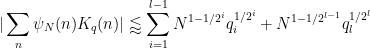Then for any ${N > 0}$ of polynomial size, any factorisation ${q = q_1 \ldots q_l}$ , and any coefficient sequence function ${\psi_N(n)}$ which is smooth at scale ${N}$ , one has

$\displaystyle |\sum_n \psi_N(n) K_q(n)| \lessapprox q_0 (1 + \sum_{i=1}^{l-1} (N')^{1-1/2^i} (q'_i)^{1/2^i}$

$\displaystyle + (N')^{1-1/2^{l-1}} (q'_l)^{1/2^l})+ N (q')^{-1/2}$

where ${q' := q / q_0}$ , ${N' := N/q_0}$ , and ${q'_i := (q_i,q')}$ , where the sum is implicitly assumed to range over those ${n}$ for which ${K_q(n)}$ is defined.

The ${q_0}$ parameter is technical, as is the ${1}$ term; heuristically one should view this estimate as asserting that

$\displaystyle |\sum_n \psi_N(n) K_q(n)| \lessapprox \sum_{i=1}^{l-1} N^{1-1/2^i} q_i^{1/2^i} + N^{1-1/2^{l-1}} q_l^{1/2^l}$

under reasonable non-degeneracy conditions. Assuming sufficient dense divisibility and in the regime ${N \geq q^{1/(l+1)}}$ , the optimal value of the right-hand side is ${\epsilon N}$ , where ${\epsilon := (q/N^{l+1})^{1/(2^{l+1}-2)}}$ , which is attained when ${q_i := N \epsilon^{2^i}}$ for ${i=1,\ldots,l-1}$ and ${q_{l} := q_{l-1}^2}$ .

Proof: We induct on ${l}$ , assuming that the claim has already been proven for all smaller values of ${l}$ .

We may factor ${K_q = K_{q_0} K_{q'}}$ where ${K_{q_0} := \prod_{p|q_0} K_p}$ and ${K_{q'} := \prod_{p|q'} K_p}$ . Then we may write

$\displaystyle \sum_n \psi_N(n) K_q(n) = \sum_{a=0}^{q_0-1} K_{q_0}(a) \sum_n \psi_N( q_0 n + a ) K_{q'}(q_0n+a).$

Observe that any given ${a}$ , ${K_{q_0}(a)}$ has magnitude ${|K_{q_0}(a)| \lessapprox 1}$ (from the divisor bound), the function ${n \mapsto \psi_N(q_0n+a)}$ is of the form ${\tilde \psi( \frac{n}{N'} )}$ for some ${\tilde \psi}$ supported on an interval of length ${\lessapprox 1}$ and obeying the bounds ${|\nabla^j \tilde \psi(x)| \lessapprox 1}$ , and the function ${n \mapsto K_{q'}(q_0 n+a)}$ is a structured function of modulus ${q'}$ and complexity at most ${O(1)}$ (here we use the dilation and translation invariance properties of structured functions). From this we see that to prove the proposition for a given value of ${l}$ , it suffices to do so under the assumption ${q_0=1}$ , in which case the objective is to prove that

$\displaystyle |\sum_n \psi_N(n) K_q(n)| \lessapprox 1 + \sum_{i=1}^{l-1} N^{1-1/2^i} q_i^{1/2^i} + N^{1-1/2^{l-1}} q_l^{1/2^l}$

$\displaystyle + N q^{-1/2} 1_{N \geq A q}.$

The claim is trivial (from the divisor bound) with ${N \leq 1}$ , so we may assume ${N \geq 1}$ , in which case we will show that

$\displaystyle |\sum_n \psi_N(n) K_q(n)| \lessapprox \sum_{i=1}^{l-1} N^{1-1/2^i} q_i^{1/2^i} + N^{1-1/2^{l-1}} q_l^{1/2^l}$

$\displaystyle + N q^{-1/2} 1_{N \geq A q}.$

By applying a similar reduction to before we may also assume that all prime factors of ${q}$ are larger than some large fixed constant ${C}$ , which we will assume to be sufficiently large for the arguments below to work.

We begin with the base case ${l=1}$ . In this case it will suffice to establish the bound

$\displaystyle |\sum_n \psi_N(n) K_q(n)| \lessapprox q^{1/2} + N q^{-1/2}.$

By completion of sums, it will suffice to show that

$\displaystyle \sum_{n \in {\bf Z}/q{\bf Z}} e_q( hn) K_q(n)| \lessapprox q^{1/2}$

for all ${h \in {\bf Z}/q{\bf Z}}$ . By the Chinese remainder theorem and the divisor bound, it will suffice to show that

$\displaystyle \sum_{n \in {\bf Z}/p{\bf Z}} e_p( hn) K_p(n)| \ll p^{1/2}$

for all ${p|q}$ and all ${h \in {\bf Z}/q{\bf Z}}$ . However, by the hypothesis ${q_0=1}$ , ${e_p(h \cdot) K_p \not \equiv 1}$ , and the claim now follows from the almost orthogonality properties of structured functions.

Now suppose that ${l > 1}$ , and the claim has already been proven for smaller values of ${l}$ . If ${N \geq q}$ then the claim follows from the ${l=1}$ bound, so we may assume that ${N < q}$ , in which case we will establish

$\displaystyle |\sum_n \psi_N(n) K_q(n)| \lessapprox \sum_{i=1}^{l-1} N^{1-1/2^i} q_i^{1/2^i} + N^{1-1/2^{l-1}} q_l^{1/2^l}.$

If we have ${N \geq q_l}$ , then

$\displaystyle N^{1-1/2^{l-1}} q_{l-1}^{1/2^{l-1}} + N^{1-1/2^{l-1}} q_l^{1/2^l} \geq N^{1-1/2^{l-2}} (q_{l-1} q_l)^{1/2^{l-1}}$

and the claim then follows by the induction hypothesis (concatenating ${q_l}$ and ${q_{l-1}}$ ). Similarly, if ${N \leq q_1}$ , then ${N^{1/2} q_1^{1/2} \geq N}$ , and the claim follows from the triangle inequality. Thus we may assume that

$\displaystyle q_1 < N < q_l.$

Let ${M := \lfloor N/q_1\rfloor}$ . We can rewrite ${\sum_n \psi_N(n) K_q(n)}$ as

$\displaystyle \frac{1}{M} \sum_n \sum_{m=1}^M \psi_N(n+kq_1) K_q(n+mq_1).$

We factor

$\displaystyle K_q(n+mq_1) = K_{q_1}(n) K_{q_2 \ldots q_l}(n+mq_1)$

and by the divisor bound ${|K_{q_1}(n)| \lessapprox 1}$ , and so by the triangle inequality and the Cauchy-Schwarz inequality

$\displaystyle |\sum_n \psi_N(n) K_q(n)| \lessapprox \frac{1}{M} \sum_n |\sum_{m=1}^M \psi_N(n+mq_1) K_{q_2 \ldots q_l}( n+mq_1 )|$

$\displaystyle \lessapprox \frac{N^{1/2}}{M} (\sum_n |\sum_{m=1}^M \psi_N(n+mq_1) K_{q_2 \ldots q_l}( n+mq_1 )|^2)^{1/2}$

since the summand is only non-zero when ${n}$ is supported on an interval of length ${\lessapprox N}$ . This last expression may be rearranged as

$\displaystyle \frac{N^{1/2}}{M} |\sum_{1 \leq m,m' \leq M} \sum_n \psi_N(n+mq_1) \overline{\psi_N(n+m'q_1)}$

$\displaystyle K_{q_2 \ldots q_l}( n+mq_1 ) \overline{K_{q_2 \ldots q_l}}(n+m'q_1)|^{1/2}.$

The diagonal contribution ${m=m'}$ can be estimated (using the pointwise bounds ${|K_{q_2\ldots q_l}| \lessapprox 1}$ ) by ${\lessapprox \frac{N^{1/2}}{M} ( M N )^{1/2} \lessapprox N^{1/2} q_1^{1/2}}$ , which is acceptable, so it suffices to show that

$\displaystyle |\sum_{1 \leq m,m' \leq M: m \neq m'} \sum_n \psi_N(n+mq_1) \overline{\psi_N(n+m'q_1)} \ \ \ \ \ (9)$

$\displaystyle K_{q_2 \ldots q_l}( n+mq_1 )\overline{K_{q_2 \ldots q_l}}(n+m'q_1) |$

$\displaystyle \lessapprox M^2 ( \sum_{i=2}^{l-1} N^{1-1/2^{i-1}} q_i^{1/2^{i-1}} + N^{1-1/2^{l-2}} q_l^{1/2^{l-1}} ).$

We observe that ${n \mapsto K_{q_2 \ldots q_l}( n+mq_1 )\overline{K_{q_2 \ldots q_l}}(n+m'q_1)}$ is the sum of ${\lessapprox 1}$ structured functions of modulus ${q_2 \ldots q_l}$ and complexity ${O(1)}$ , each of which the product of one of the components of ${K_p( n+mq_1) \overline{K_p}(n+m'q_1)}$ of modulus ${p}$ and complexity ${O(1)}$ for all ${p|q_2 \ldots q_l}$ . We can of course delete any components that vanish identically. Suppose that for one of these primes ${p}$ , one of the components of the function ${K_p( n+mq_1) \overline{K_p}(n+m'q_1)}$ is equivalent to ${e_p( P(n) )}$ for some polynomial ${P}$ of degree at most ${l-1}$ . Then by Lemma 10, if ${p}$ is sufficiently large (larger than a fixed constant), either ${p|m'-m}$ , or else ${K_p(n)}$ is equivalent ${e_p(Q)}$ for some polynomial ${Q}$ of degree at most ${l}$ , but by the hypothesis ${q_0=1}$ the latter case cannot occur since ${K_p}$ is non-vanishing and ${c_{K_p,e_p(Q)} = 0}$ . Thus if we set ${\tilde q_0}$ to be the product of all the primes ${p}$ with this property, we see that ${\tilde q_0 \ll (m'-m,q_2 \ldots q_l)}$ .

Applying the induction hypothesis, we may thus bound

$\displaystyle |\sum_n \psi_N(n+mq_1) \overline{\psi_N(n+m'q_1)} K_{q_2 \ldots q_l}( n+ mq_1) \overline{K_{q_2 \ldots q_l}}( n+ m'q_1)$

$\displaystyle \lessapprox (q_2 \ldots q_l, m-m') [ \sum_{i=2}^{l-1} N^{1-1/2^{i-1}} q_i^{1/2^{i-1}} + N^{1-1/2^{l-2}} q_l^{1/2^{l-1}} ]$

$\displaystyle + N (q_2 \ldots q_l)^{-1/2} (q_2 \ldots q_l, m-m')^{1/2}.$

The contribution of the first two terms to (9) is acceptable thanks to Lemma 5 of this previous post, so the only contribution remaining to control is

$\displaystyle \sum_{1 \leq m,m' \leq M: m \neq m'} N (q_2 \ldots q_l)^{-1/2} (q_2 \ldots q_l, m-m')^{1/2}.$

We may bound

$\displaystyle N (q_2 \ldots q_l)^{-1/2} (q_2 \ldots q_l, m-m')^{1/2} \ll N^{1/2} + N^{3/2} (q_2 \ldots q_l)^{-1} (q_2 \ldots q_l, m-m').$

The first term is dominated by the ${N^{1/2} q_1^{1/2}}$ term appearing as the ${i=1}$ summand in (9), while the contribution of the second term may be bounded using another application of Lemma 5 of this previous post and the bound ${N < q_l}$ by

$\displaystyle \lessapprox K^2 N^{1-1/2^{l-2}} q_l^{1/2^{l-1}}$

which is acceptable. $\Box$

Remark 1 The above arguments relied on a ${q}$ -version of the van der Corput ${A}$ -process, and in the case of Dirichlet characters is essentially due to Graham and Ringrose (see also Heath-Brown). If we work with a class of structured functions that is closed under Fourier transforms (such as the trace weights), then the ${q}$ -version of the van der Corput ${B}$ -process also becomes available (in principle, at least), thus potentially giving a slightly larger range of “exponent pairs”; however this looks complicated to implement (the role of polynomial phases now needs to be replaced by a more complicated class that involves things like the Fourier transforms of polynomial phases, as well as their “antiderivatives”) and will likely only produce rather small improvements in the final numerology.

We isolate a special case of the above result:

Corollary 12 Let the notation and assumptions be as in Proposition 11 with ${l=2}$ , ${N \geq 1}$ , and ${q}$ ${y}$ -densely divisible. Then for any ${N > 0}$ , one has the bounds

$\displaystyle |\sum_n \psi_N(n) K_q(n)| \lessapprox q_0 + q_0^{1/2} q^{1/2} + N q_0^{1/2} q^{-1/2}$

and

$\displaystyle |\sum_n \psi_N(n) K_q(n)| \lessapprox q_0 + q_0^{1/2} N^{1/2} q^{1/6} y^{1/6} + N q_0^{1/2} q^{-1/2}.$

The dependence on ${q_0}$ in the first bound can be improved, but we will not need this improvement here.

Proof: From the ${l=1}$ case of the above proposition we have

$\displaystyle |\sum_n \psi_N(n) K_q(n)| \lessapprox q_0 (1 + (q/q_0)^{1/2}) + N (q/q_0)^{-1/2}$

giving the first claim of the proposition.

Similarly, from the ${l=2}$ case of the above proposition we have

$\displaystyle |\sum_n \psi_N(n) K_q(n)| \lessapprox q_0 (1 + (N')^{1/2} (q_1)^{1/2} + (N')^{1/2} (q_2)^{1/4} )$

$\displaystyle + N q_0^{1/2} q^{-1/2}$

for any factorisation ${q=q_1q_2}$ of ${q}$ . As ${q}$ is ${y}$ -densely divisible, we may select ${q_1}$ so that

$\displaystyle y^{-2/3} q^{1/3} \leq q_1 \leq y^{1/3} q^{1/3}$

so that

$\displaystyle y^{-1/3} q^{2/3} \leq q_2 \leq y^{2/3} q^{2/3}$

and the second claim follows. $\Box$

— 3. A two-dimensional exponential sum —

We now apply the above theory to obtain a new bound on a certain two-dimensional exponential sum that will show up in the Type I estimate.

Proposition 13 Let ${u}$ be a ${y}$ -densely divisible squarefree integer of polynomial size for some ${y \geq 1}$ , let ${D, N > 0}$ be of polynomial size, and let ${c,l,v,a,b \in {\bf Z}/u{\bf Z}}$ . Let ${\psi_D, \psi_N}$ be smooth sequences at scale ${D, N}$ respectively. Then

$\displaystyle |\sum_d \sum_n \psi_D(d) \psi_N(n) e_u( \frac{cl}{(n+vd+a)(n+vd+ld+b)} )|$

$\displaystyle \lessapprox (cl,u) (u^{1/2} + \frac{N}{u^{1/2}}) ( 1 + D^{1/2} u^{1/6} y^{1/6} + \frac{D}{u^{1/2}}).$

Here the summations are implicitly restricted to those ${d,n}$ for which the denominator in the phase is non-zero. We also have the bound

$\displaystyle |\sum_d \sum_n \psi_D(d) \psi_N(n) e_u( \frac{cl}{(n+vd+a)(n+vd+ld+b)} )|$

$\displaystyle \lessapprox (cl,u) ( u^{1/2} + \frac{N}{u^{1/2}}) ( u^{1/2} + \frac{D}{u^{1/2}}).$

The main term here is ${(cl,u) u^{1/2} \times (D^{1/2} u^{2/3} y^{1/6})}$ , which in certain regimes improves upon the bound of ${((cl,u)^{-1/2} u^{1/2}) \times D}$ that one obtains by completing the sums in the ${n}$ variable but not exploiting any additional cancellation in the ${d}$ variable.

Proof: We first claim that it suffices to verify the proposition when ${(cl,u)=1}$ . Indeed, if we set

$\displaystyle u' := u / (cl,u)$

$\displaystyle y' := y (cl,u)$

$\displaystyle c' := c/(cl,u) = \frac{c/(c,u)}{(cl,u)/(c,u)}$

(where one computes the reciprocal of ${(cl,u)/(c,u)}$ inside ${{\bf Z}/(u/(cl,u)){\bf Z}}$ ), we see that ${u'}$ is ${y'}$ -densely divisible (thanks to Lemma 7), squarefree, and polynomial size, that ${(c'l,u')=1}$ , and that

$\displaystyle \sum_d \sum_n \psi_D(d) \psi_N(n) e_u( \frac{cl}{(n+vd+a)(n+vd+ld+b)} )$

$\displaystyle = \sum_d \sum_n \psi_D(d) \psi_N(n) e_{u'}( \frac{c'l}{(n+vd+a)(n+vd+ld+b)} )$

$\displaystyle \prod_{p|(cl,u)} 1_{p \not | (n+vd+a)(n+vd+ld+b)}.$

By the inclusion-exclusion formula and divisor bound, it thus suffices to show that for all ${f | (cl,u)}$ , one has

$\displaystyle |\sum_d \sum_n \psi_D(d) \psi_N(n) e_{u'}( \frac{c'l}{(n+vd+a)(n+vd+ld+b)} )$

$\displaystyle 1_{f|(n+vd+a)(n+vd+ld+b)}| \lessapprox X$

where ${X}$ is either of the two right-hand sides in the proposition, i.e. either

$\displaystyle X = (cl,u) (u^{1/2} + \frac{N}{u^{1/2}})$

$\displaystyle X = (cl,u) ( u^{1/2} + \frac{N}{u^{1/2}}) ( u^{1/2} + \frac{D}{u^{1/2}}).$

By the divisor bound, we see that there are ${\lessapprox f}$ pairs ${(n_0,d_0) \in ({\bf Z}/f{\bf Z})^2}$ such that ${(n_0+vd_0+a)(n_0+vd_0+ld_0+b) = 0\ (f)}$ . Thus it will suffice to show that

$\displaystyle |\sum_{d=d_0\ (f)} \sum_{n=n_0\ (f)} \psi_D(d) \psi_N(n) e_{u'}( \frac{c'l}{(n+vd+a)(n+vd+ld+b)} )| \lessapprox X/f.$

Making the change of variables ${d = fd' +d_0}$ , ${n = fn'+n_0}$ and using the ${(cl,u)=1}$ case of the proposition, we can bound the left-hand side by

$\displaystyle ((u')^{1/2} + \frac{N/f}{(u')^{1/2}}) ( 1 + (D/f)^{1/2} (u')^{1/6} (y')^{1/6} + \frac{D/f}{(u')^{1/2}})$

and

$\displaystyle ((u')^{1/2} + \frac{N/f}{(u')^{1/2}}) ( (u')^{1/2} + \frac{D/f}{(u')^{1/2}})$

and one verifies that these two quantities bound the two possible values of ${X/f}$ respectively.

Henceforth ${(cl,u)=1}$ . Note that the above reduction also allows us to assume that ${u}$ has no prime factors less than a sufficiently large fixed constant ${C}$ to be chosen later. Our task is now to show that

$\displaystyle |\sum_d \sum_n \psi_D(d) \psi_N(n) e_u( \frac{cl}{(n+vd+a)(n+vd+ld+b)} )|$

$\displaystyle \lessapprox (\frac{N}{u}+1) (u^{1/2} + D^{1/2} u^{2/3} y^{1/6} + D)$

and

$\displaystyle |\sum_d \sum_n \psi_D(d) \psi_N(n) e_u( \frac{cl}{(n+vd+a)(n+vd+ld+b)} )|$

$\displaystyle \lessapprox (\frac{N}{u}+1) (u + D).$

From completion of sums we have

$\displaystyle |\sum_d \sum_n \psi_D(d) \psi_N(n) e_u( \frac{cl}{(n+vd+a)(n+vd+ld+b)} )|$

$\displaystyle \lessapprox (\frac{N}{u}+1) \sup_{m \in{\bf Z}/u{\bf Z}} |\sum_d \sum_{n \in {\bf Z}/u{\bf Z}} \psi_D(d)$

$\displaystyle e_u( \frac{cl}{(n+vd+a)(n+vd+ld+b)} + mn)|$

so it will suffice to show that

$\displaystyle |\sum_d \sum_{n \in {\bf Z}/u{\bf Z}} \psi_D(d) e_u( \frac{cl}{(n+vd+a)(n+vd+ld+b)} + mn)|$

$\displaystyle \lessapprox u^{1/2} + D^{1/2} u^{2/3} y^{1/6} + D$

and

$\displaystyle |\sum_d \sum_{n \in {\bf Z}/u{\bf Z}} \psi_D(d) e_u( \frac{cl}{(n+vd+a)(n+vd+ld+b)} + mn)|$

$\displaystyle \lessapprox u + D$

for any given ${m \in {\bf Z}/u{\bf Z}}$ . We rewrite this as

$\displaystyle |\sum_d \psi_D(d) K_u(d)| \lessapprox \min( 1 + D^{1/2} u^{1/6} y^{1/6}, u^{1/2}) + D u^{-1/2} \ \ \ \ \ (10)$

where

$\displaystyle K_u(d) := \frac{1}{\sqrt{u}} \sum_{n \in {\bf Z}/u{\bf Z}} e_u( \frac{cl}{(n+vd+a)(n+vd+ld+b)} + mn).$

By the Chinese remainder theorem, this function factors as ${K_u(d) = \prod_{p|u} K_p(d)}$ , where

$\displaystyle K_p(d) := \frac{1}{\sqrt{p}} \sum_{n \in {\bf Z}/p{\bf Z}} e_p( \frac{1}{u_p} ( \frac{cl}{(n+vd+a)(n+vd+ld+b)} + mn ) )$

and ${u_p := u/p}$ . Note that for any prime ${p}$ dividing ${u}$ (and thus larger than ${C}$ ), the rational function ${n \mapsto \frac{1}{u_p} ( \frac{cl}{n(n+ld+b-a)} + mn )}$ is not divisible by ${p}$ . From the Weil conjectures for curves this implies that ${K_p(d) = O(1)}$ . In fact, from Deligne’s theorem (and in particular the fact that cohomology groups of sheaves are again sheaves), we have the stronger assertion that ${K_p}$ is a sum of boundedly many trace weights at modulus ${p}$ with complexity ${O(1)}$ in the sense of Example 4. (In the Grothendieck-Lefschetz trace formula, only the first cohomology ${H^1_c}$ is non-trivial; the second cohomology ${H^2_c}$ disappears because the rational function is not divisible by ${p}$ , and the zeroth cohomology ${H^0_c}$ disappears because the underlying curve is affine, although in any event the contribution of the zeroth cohomology could be absorbed into the ${Du^{-1/2}}$ term in (10).) By the divisor bound, this implies that ${K_u}$ is the sum of ${\lessapprox 1}$ trace weights at modulus ${u}$ with complexity ${O(1)}$ . We can of course delete any components that vanish identically.

We claim that for any ${p}$ dividing ${u}$ (and hence larger than ${C}$ ), none of the components of ${K_p(d)}$ are equivalent to a quadratic phase ${e_p( ed^2+fd )}$ . Assuming this claim for the moment, the required bound (10) then follows from Corollary 12. It thus suffices to verify the claim. If the claim failed, then we would have

$\displaystyle \sum_{d \in {\bf Z}/p{\bf Z}} K_p(d) e_p( - ed^2 - fd ) = \alpha p + O(\sqrt{p}) \ \ \ \ \ (11)$

for some algebraic integer ${\alpha}$ , which is non-zero since ${K_p(d)}$ is equivalent to ${e_p(ed^2+f d)}$ and is non-zero. Since all non-zero algebraic integers have at least one Galois conjugate of modulus at least ${1}$ , it will suffice (for ${p}$ large enough) to establish that all Galois conjugates of the left-hand side of (27) are ${O(\sqrt{p})}$ . In other words, it suffices to establish the bound

$\displaystyle |\sum_{d,n \in {\bf Z}/p{\bf Z}} e_p( g ( \frac{1}{u_p} ( \frac{cl}{(n+vd+a)(n+vd+ld+b)} + mn ) - ed^2 - fd ) )|$

$\displaystyle \ll p$

for all ${g \in ({\bf Z}/p{\bf Z})^\times}$ . Setting ${x := n+vd+a}$ and ${y := ld+b}$ and concatenating parameters, it suffices to show that

$\displaystyle |\sum_{x,y \in {\bf Z}/p{\bf Z}} e_p( \frac{c}{x (x+y)} - ax - by - dy^2 )| \ll p$

whenever ${c \in ({\bf Z}/p{\bf Z})^\times}$ and ${a,b,d \in {\bf Z}/p{\bf Z}}$ .

We now use a result of Hooley, which asserts that for any rational function ${f(x,y)}$ of two variables and bounded degree, one has

$\displaystyle |\sum_{x,y \in {\bf Z}/p{\bf Z}} e_p( f(x,y) )| \ll p$

provided that

$\displaystyle \{ (x,y): f(x,y)-T = 0\}$

is a geometrically generically irreducible curve (i.e. irreducible over an algebraic closure ${k := \overline{{\Bbb F}_p(T)}}$ of ${k_0 := {\Bbb F}_p(T)}$ ) and also that

$\displaystyle \{ (x,y): f(x,y)-t = 0 \}$

is a (possibly reducible or empty) curve for any ${t \in \overline{F}_p}$ . We apply this result to the rational function

$\displaystyle f(x,y) := \frac{c}{x (x+y)} - ax - by - dy^2.$

For any ${t}$ , it is clear that ${f(x,y)-t}$ is not identically zero, so the second condition of Hooley is satisfied. It remains to verify the first. (Thanks to Brian Conrad for fixing some errors in the argument that follows.) Suppose that the claim failed, thus ${f(x,y)-T}$ is reducible for generic ${T}$ , or equivalently that the polynomial

$\displaystyle P(x,y) := c - (ax + by + dy^2 - T) (x(x+y))$

is reducible in ${k[x,y]}$ . Being linear in ${T}$ , this polynomial ${P}$ is clearly irreducible in ${{\Bbb F}_p[x,y,T] = {\Bbb F}_p[T][x,y]}$ ; since ${P}$ does not lie in ${{\Bbb F}_p[T]}$ , it remains irreducible in the larger ring ${k_0[x,y]}$ by Gauss’s lemma.

We now perform a technical reduction to deal with the problem that the field ${k_0}$ is not perfect. Since ${P}$ involves the nonzero term ${Txy}$ as its only ${xy}$ -term, over ${k}$ it cannot be a constant multiple of a ${p}$ -power. Hence, if it is irreducible over the separable closure ${k_{0,s}}$ of ${k_0}$ then it remains irreducible over the perfect closure ${k}$ of ${k_{0,s}}$ , so it suffices to check irreducibility over the separable closure.

Assuming ${P}$ is reducible over the separable closure, then up to constant multipliers (i.e. multiples in ${k_{0,s}}$ ) its irreducible factors in ${k_{0,s}[x,y]}$ must be Galois conjugate to each other with respect to ${{\rm{Gal}}(k_{0,s}/k_0)}$ . Thus, none of these factors can lie in ${k_{0,s}[x]}$ or ${k_{0,s}[y]}$ , as otherwise all the factors would and hence so would their product ${P}$ (a contradiction since ${c \ne 0}$ ). Thus, the irreducible factorization over ${k_{0,s}[x,y]}$ remains an irreducible factorization in ${k_{0,s}(x)[y]}$ and over ${k_{0,s}(y)[x]}$ . Since ${P}$ has nonzero constant term and degree at most ${3}$ in either ${x}$ or ${y}$ , this implies that the irreducible factors of ${P}$ in ${k[x,y]}$ are linear in both ${x}$ and ${y}$ , thus

$\displaystyle P(x,y) = \prod_{i=1}^3 (\alpha_i x + \beta_i y + \gamma_i)$

for some ${\alpha_i, \beta_i \in k}$ and ${\gamma_i \in k^{\times}}$ . But ${P(0,y)}$ is visibly constant, so all ${\beta_i}$ vanish and hence ${P \in k[x]}$ , an absurdity. $\Box$

— 4. Type I estimate —

We begin the proof of Theorem 4, closely following the arguments from Section 5 of this previous post or Section 2 of this previous post. One difference however will be that we will not discard the ${r}$ averaging as we will need it near the end of the argument. Let ${I, a, N, M, \alpha}$ be as in the theorem. We can restrict ${q}$ to the range

$\displaystyle q \gtrapprox x^{1/2}$

for some sufficiently slowly decaying ${o(1)}$ , since otherwise we may use the Bombieri-Vinogradov theorem (Theorem 4 from this previous post). Thus, by dyadic decomposition, we need to show that

$\displaystyle \sum_{d \in {\mathcal S}_I \cap {\mathcal D}_{x^\delta}^4: D \leq d < 2D} |\Delta(\alpha \ast \beta; a\ (d))| \ll NM \log^{-A} x. \ \ \ \ \ (12)$

for any fixed ${A}$ and for any ${D}$ in the range

$\displaystyle x^{1/2} \lessapprox D \lessapprox x^{1/2+2\varpi}.$

Let

$\displaystyle \epsilon > 0 \ \ \ \ \ (13)$

be a sufficiently small fixed exponent.

By Lemma 11 of this previous post, we know that for all ${d}$ in ${[D,2D]}$ outside of a small number of exceptions, we have

$\displaystyle \prod_{p|d: p \leq D_0} p \lessapprox 1 \ \ \ \ \ (14)$

where

$\displaystyle D_0 := \exp(\log^{1/3} x). \ \ \ \ \ (15)$

Specifically, the number of exceptions in the interval ${[D,2D]}$ is ${O(D \log^{-A} x)}$ for any fixed ${A>0}$ . The contribution of the exceptional ${d}$ can be shown to be acceptable by Cauchy-Schwarz and trivial estimates (see Section 5 of this previous post), so we restrict attention to those ${d}$ for which (14) holds. In particular, as ${d}$ is restricted to be quadruply ${x^\delta}$ -densely divisible, we may factor

$\displaystyle d=qr$

with ${q,r}$ coprime and square-free, with ${q \in {\mathcal S}_{I'}}$ ${x^{\delta+o(1)}}$ -densely divisible with ${I' := [D_0,\infty) \cap I}$ , ${r \in {\mathcal S}_I}$ doubly ${x^{\delta+o(1)}}$ -densely divisible,and

$\displaystyle x^{-\epsilon-\delta} N \lessapprox r \lessapprox x^{-\epsilon} N$

and

$\displaystyle x^{1/2} \lessapprox qr \lessapprox x^{1/2+2\varpi}.$

Here we use the easily verified fact that ${N \gtrapprox x^\epsilon}$ , and we have also used Lemma 7 to ensure that dense divisibility is essentially preserved when transferring a factor of ${x^{o(1)}}$ from ${r}$ (namely, the portion of ${r}$ coming from primes up to ${D_0}$ ) to ${q}$ .

By dyadic decomposition, it thus suffices to show that

$\displaystyle \sum_{q \in {\mathcal S}_{I'} \cap {\mathcal D}_{x^\delta+o(1)}: q \sim Q} \sum_{r \in {\mathcal S}_I \cap {\mathcal D}_{x^\delta+o(1)}^{(2)}: r \sim R} |\Delta(\alpha \ast \beta; a\ (qr))| \ll NM \log^{-A} x.$

for any fixed ${A>0}$ , where ${Q, R \geq 1}$ obey the size conditions

$\displaystyle x^{-\epsilon-\delta} N \lessapprox R \lessapprox x^{-\epsilon} N \ \ \ \ \ (16)$

and

$\displaystyle x^{1/2} \lessapprox QR \lessapprox x^{1/2 + 2\varpi}. \ \ \ \ \ (17)$

Fix ${Q,R}$ . We abbreviate ${\sum_{q \in {\mathcal S}_{I'} \cap {\mathcal D}_{x^\delta+o(1)}: q \sim Q}}$ and ${\sum_{r \in {\mathcal S}_I \cap {\mathcal D}_{x^{\delta+o(1)}}^2: r \sim R}}$ by ${\sum_q}$ and ${\sum_r}$ respectively, thus our task is to show that

$\displaystyle \sum_q \sum_{r: (q,r)=1} |\Delta(\alpha \ast \beta; a\ (qr))| \ll NM \log^{-A} x.$

We now split the discrepancy

$\displaystyle \Delta(\alpha \ast \beta; a\ (qr)) = \sum_{n = a\ (qr)} \alpha \ast \beta(n) - \frac{1}{\phi(qr)} \sum_{n: (n,qr)=1} \alpha \ast \beta(n)$

as the sum of the subdiscrepancies

$\displaystyle \sum_{n: n = a\ (qr)} \alpha \ast \beta(n) - \frac{1}{\phi(q)} \sum_{n: (n,q)=1; n = a\ (r)} \alpha \ast \beta(n)$

and

$\displaystyle \frac{1}{\phi(q)} \sum_{n: (n,q)=1; n = a\ (r)} \alpha \ast \beta(n) - \frac{1}{\phi(qr)} \sum_{n: (n,qr)=1} \alpha \ast \beta(n).$

In Section 5 of this previous post, it was established (using the Bombieri-Vinogradov theorem) that

$\displaystyle \sum_{q} \sum_{r; (q,r)=1} |\frac{1}{\phi(q)} \sum_{n: (n,q)=1; n = a\ (r)} \alpha \ast \beta(n) - \frac{1}{\phi(qr)} \sum_{n: (n,qr)=1} \alpha \ast \beta(n)|$

$\displaystyle NM \log^{-A} x$

so it suffices to show that

$\displaystyle \sum_{q} \sum_{r; (q,r)=1} |\sum_{n: n = a\ (qr)} \alpha \ast \beta(n) - \frac{1}{\phi(q)} \sum_{n: (n,q)=1; n = a\ (r)} \alpha \ast \beta(n)| \ \ \ \ \ (18)$

$\displaystyle \ll NM \log^{-A} x.$

It will suffice to prove the slightly stronger statement

$\displaystyle \sum_r \sum_{q: (q,r)=1} |\sum_{n: n = a\ (r); n= b\ (q)} \alpha \ast \beta(n) - \sum_{n: (n,q)=1; n = a\ (r); n = b'\ (q)} \alpha \ast \beta(n)| \ \ \ \ \ (19)$

$\displaystyle \ll NM \log^{-A} x$

for all ${a,b,b'}$ coprime to ${P_I}$ , since if one then specialises to the case when ${b=a}$ and averages over all primitive ${b'\ (P_I)}$ we obtain (18) from the triangle inequality.

We use the dispersion method. We write the left-hand side of (19) as

$\displaystyle \sum_r \sum_{q: (q,r)=1} c_{q,r} (\sum_{n: n = a\ (r); n= b\ (q)} \alpha \ast \beta(n) - \sum_{n: n = a\ (r); n = b'\ (q)} \alpha \ast \beta(n))$

for some bounded sequence ${c_{q,r}}$ . This expression may be rearranged as

$\displaystyle \sum_r \sum_m \alpha(m) (\sum_{q,n: mn = a\ (r); (q,r)=1} c_{q,r} \beta(n) (1_{mn = b\ (q)} - 1_{mn = b'\ (q)})),$

so from the Cauchy-Schwarz inequality and crude estimates it suffices to show that

$\displaystyle \sum_r \sum_{m} \psi_M(m) |\sum_{q,n: mn = a\ (r); (q,r)=1} c_{q,r} \beta(n) (1_{mn = b\ (q)} - 1_{mn = b'\ (q)})|^2 \ \ \ \ \ (20)$

$\displaystyle \ll N^2 M R^{-1} \log^{-A} x$

for any fixed ${A>0}$ , where ${\psi_M}$ is a smooth coefficient sequence at scale ${M}$ . Expanding out the square, it suffices to show that

$\displaystyle \sum_r \sum_{m} \psi_M(m) \sum_{q_1,q_2,n_1,n_2: mn_1=mn_2 = a\ (r); (q_1q_2,r)=1} \ \ \ \ \ (21)$

$\displaystyle c_{q_1,r} \overline{c_{q_2,r}} \beta(n_1) \overline{\beta(n_2)} 1_{mn_1 = b\ (q_1)} 1_{mn_2 = b'\ (q_2)}$

$\displaystyle = X + O( N^2 M R^{-1} \log^{-A} x )$

where ${q_1,q_2}$ is subject to the same constraints as ${q}$ (thus ${q_i \in {\mathcal S}_{I'} \cap {\mathcal D}_{x^\delta}}$ and ${q_i \sim Q}$ for ${i=1,2}$ ), and ${X}$ is some quantity that is independent of ${b,b'}$ .

Observe that ${n_1}$ must be coprime to ${q_1r}$ and ${n_2}$ coprime to ${q_2r}$ , with ${n_1 = n_2\ (r)}$ , to have a non-zero contribution to (21). We then rearrange the left-hand side as

$\displaystyle \sum_r \sum_{q_1,q_2: (q_1q_2,r)=1} \sum_{m} \psi_M(m) \sum_{n_1,n_2: n_1=n_2\ (r); (n_1,q_1r)=(n_2,q_2)=1}$

$\displaystyle c_{q_1,r} \overline{c_{q_2,r}} \overline{\beta(n_1)} \overline{\beta(n_2)} 1_{m = a/n_1\ (r); m = b/n_1\ (q_1); m = b'/n_2 (q_2)};$

note that these inverses in the various rings ${{\bf Z}/r{\bf Z}}$ , ${{\bf Z}/q_1{\bf Z}}$ , ${{\bf Z}/q_2{\bf Z}}$ are well-defined thanks to the coprimality hypotheses.

We may write ${n_2 = n_1+kr}$ for some ${k = O(N/R)}$ . By the triangle inequality, and relabeling ${n_1}$ as ${n}$ , it thus suffices to show that

$\displaystyle \sum_r \sum_{k = O(N/R)} \sum_{q_1,q_2: (q_1q_2,r)=1} |\sum_{n; (n,q_1r)=(n+kr,q_2)=1} \ \ \ \ \ (22)$

$\displaystyle c_{q_1} \overline{c_{q_2}} \beta(n) \overline{\beta(n+kr)} \sum_{m} \psi_M(m) 1_{m = a/n\ (r); m = b/n\ (q_1); m = b'/(n+kr) (q_2)}|$

$\displaystyle = X + O( N^2 M R^{-1} \log^{-A} x )$

for some ${X}$ independent of ${b}$ , ${b'}$ .

At this stage in previous posts we isolated the coprime case ${(q_1,q_2)=1}$ as the dominant case, using a controlled multiplicity hypothesis to deal with the non-coprime case. Here, we will carry the non-coprime case with us for a little longer so as not to rely on a controlled multiplicity hypothesis; this introduces some additional factors of ${q_0 := (q_1,q_2)}$ into the analysis but they should be ignored on a first reading.

Applying completion of sums (Section 2 from this previous post), we can express the left-hand side of (22) as a main term

$\displaystyle \sum_r \sum_{k = O(N/R)} \sum_{q_1,q_2: (q_1q_2,r)=1} |\sum_{n; (n,q_1r)=(n+kr,q_2)=1} \ \ \ \ \ (23)$

$\displaystyle c_{q_1,} \overline{c_{q_2,r}} \beta(n) \overline{\beta(n+kr)} (\sum_{m} \psi_M(m)) \frac{1}{r[q_1,q_2]} 1_{b/n = b'/(n+kr)\ ((q_1,q_2))}$

plus an error term

$\displaystyle O( \frac{1}{H} \sum_r \sum_{k=O(N/R)} \sum_{1 \leq h \leq H} \sum_{q_1,q_2} |\sum_{n} \beta(n) \beta(n+kr) \Phi_{k,r}(h,q_1,q_2; n)| ) \ \ \ \ \ (24)$

$\displaystyle + O( x^{-A} ),$

where

$\displaystyle H := x^\epsilon Q^2 R/M \ \ \ \ \ (25)$

and ${\Phi_{k,r}}$ is the phase

$\displaystyle \Phi_{k,r}(h,q_1,q_2;n) := 1_{(n,r)=(n,q_1)=(n+kr,q_2)=1} 1_{q_1,q_2 \in {\mathcal S}_I \cap {\mathcal D}_{x^{\delta+o(1)}}; (q_1q_2,r)=1} \ \ \ \ \ (26)$

$\displaystyle 1_{b/n=b'/(n+kr)\ ((q_1,q_2))}$

$\displaystyle e_r( \frac{ah}{nq_1 q'_2} ) e_{q_1}( \frac{bh}{n r q'_2} ) e_{q'_2}( \frac{b' h}{(n+kr) r q_1} ),$

where ${q'_2 := q_2/(q_1,q_2)}$ .

Let us first deal with the main term (23). The contribution of the coprime case ${(q_1,q_2)=1}$ does not depend on ${b,b'}$ and can thus be absorbed into the ${X}$ term. Now we consider the contribution of the non-coprime case when ${q_0 = (q_1,q_2) > 1}$ . We may estimate the contribution of this case by

$\displaystyle O( \sum_r \sum_{k = O(N/R)} \sum_{q_0 \in {\mathcal S}_{I'}: 1 < q_0 \ll Q, (q_0,r)=1} \sum_{q'_1,q'_2 \sim Q/q_0} |\sum_{n: b/n = b'/(n+kr)\ (q_0)}$

$\displaystyle |\beta(n)| |\beta(n+kr)| M \frac{1}{rq_0 q'_1 q'_2} ).$

We may estimate ${|\beta(n)| |\beta(n+kr)|}$ by ${|\beta(n)|^2 + |\beta(n+kr)|^2}$ . We just estimate the contribution of ${|\beta(n)|^2}$ , as the other case is treated similarly (after shifting ${n}$ by ${kr}$ ). We rearrange this contribution as

$\displaystyle O( \sum_r \sum_{q_0 \in {\mathcal S}_{I'}: 1 < q_0 \ll Q, (q_0,r)=1} \sum_{q'_1,q'_2 \sim Q/q_0} |\sum_{n}$

$\displaystyle |\beta(n)|^2 M \frac{1}{Rq_0 q'_1 q'_2} \sum_{k = O(N/R)} 1_{b/n = b'/(n+kr)\ (q_0)} ).$

The ${k}$ summation is ${O( 1 + \frac{N}{Rq_0} )}$ . Evaluating the ${n, r, q'_1,q'_2}$ summations, we obtain a bound of

$\displaystyle O( MN \log^{O(1)} x \sum_{q_0 \in {\mathcal S}_{I'}: 1 < q_0 \ll Q} \frac{1}{q_0} ( 1 + \frac{N}{Rq_0} ) ).$

Since ${q_0 > 1}$ and ${q_0 \in {\mathcal S}_{I'}}$ , we have ${q_0 \geq D_0}$ , and so we may evaluate the ${q_0}$ summation as

$\displaystyle O( MN \log^{O(1)} x (1 + \frac{N}{RD_0} ) ).$

By (16) and (15), this is ${O( N^2 M R^{-1} \log^{-A} x )}$ as required.

It remains to control (24). We may assume that ${H \geq 1}$ , as the claim is trivial otherwise. It will suffice to obtain the bound

$\displaystyle \frac{1}{H} \sum_r \sum_{k=O(N/R)} \sum_{1 \leq h \leq H} \sum_{q_1,q_2 \sim Q} |\sum_{n} \beta(n) \overline{\beta(n+kr)} \Phi_{k,r}(h,q_1,q_2; n)|$

$\displaystyle \lessapprox x^{-\epsilon} N^2 M R^{-1}.$

Using (25), it will suffice to show that

$\displaystyle \sum_r \sum_{1 \leq h \leq H} \sum_{q_1,q_2 \sim Q} |\sum_{n} \beta(n) \overline{\beta(n+kr)} \Phi_{k,r}(h,q_1,q_2; n)|$

$\displaystyle \lessapprox Q^2 N R$

for each ${k = O(N/R)}$ .

We now work with a single ${k}$ . To proceed further, we write ${q_0 := (q_1,q_2)}$ and ${q_1 = q_0 q'_1}$ , ${q_2 = q_0 q'_2}$ ; it then suffices to show that

$\displaystyle \sum_r \sum_{1 \leq h \leq H} \sum_{q'_1,q'_2 \sim Q/q_0: (q'_1,q'_2) = 1} \ \ \ \ \ (27)$

$\displaystyle |\sum_{n} \beta(n) \overline{\beta(n+kr)} \Phi_{k,r}(h,q_0 q'_1,q_0 q'_2; n)|$

$\displaystyle \lessapprox Q^2 N R / q_0$

for each ${q_0 \geq 1}$ .

Henceforth we work with a single choice of ${q_0}$ . We pause to verify the relationship

$\displaystyle H \lessapprox Q.$

From (25) and (17), this follows from the assertion that

$\displaystyle x^{1/2+2\varpi+\epsilon} \lessapprox M,$

but this follows from (4), (5) if ${\epsilon}$ is sufficiently small depending on ${c}$ .

As ${q_1}$ is ${x^{\delta+o(1)}}$ -densely divisible, we may now factor ${q_1 = s_1 t_1}$ where

$\displaystyle x^{-\delta} Q/H \lessapprox s_1 \lessapprox Q/H$

and thus

$\displaystyle H \lessapprox t_1 \lessapprox x^\delta H.$

Factoring out ${q_0}$ , we may then write ${q'_1 = s'_1 t'_1}$ where

$\displaystyle q_0^{-1} x^{-\delta} Q/H \lessapprox s'_1 \lessapprox Q/H$

and

$\displaystyle q_0^{-1} H \lessapprox t'_1 \lessapprox x^\delta H.$

By dyadic decomposition, it thus suffices to show that

$\displaystyle \sum_r \sum_{1 \leq h \leq H} \sum_{s'_1 \sim S; t'_1 \sim T; q'_2 \sim Q/q_0: (s'_1 t'_1,q'_2) = 1}$

$\displaystyle |\sum_{n} \beta(n) \overline{\beta(n+kr)} \Phi_{k,r}(h,q_0 s'_1 t'_1,q_0 q'_2; n)|$

$\displaystyle \lessapprox Q^2 N R / q_0$

whenever ${S,T}$ are such that

$\displaystyle q_0^{-1} x^{-\delta} Q/H \lessapprox S \lessapprox Q/H$

and

$\displaystyle q_0^{-1} H \lessapprox T \lessapprox x^\delta H.$

and

$\displaystyle ST \sim Q/q_0.$

We rearrange this estimate as

$\displaystyle |\sum_r \sum_{n; s'_1 \sim S; q'_2 \sim Q/q_0} \beta(n) \overline{\beta(n+kr)} \sum_{1 \leq h \leq H; t'_1 \sim T}$

$\displaystyle c_{h,s'_1,t'_1,q'_2} \Phi_{k,r}(h,q_0 s'_1 t'_1,q_0 q'_2; n)|$

$\displaystyle \lessapprox QRSTN$

for some bounded sequence ${c_{h,s_1,t_1,q_2}}$ which is only non-zero when

$\displaystyle (s'_1 t'_1,q'_2) = (q_0,s'_1t'_1) = (q_0,q'_2) = 1.$

By Cauchy-Schwarz and crude estimates, it then suffices to show that

$\displaystyle \sum_r \sum_{n; s'_1 \sim S; q'_2 \sim Q/q_0} \psi_N(n) |\sum_{1 \leq h \leq H; t'_1 \sim T} c_{h,s'_1,t'_1,q'_2} \Phi_{k,r}(h,q_0 s'_1 t'_1,q_0 q_2; n)|^2$

$\displaystyle \lessapprox QRST^2 N q_0$

where ${\psi_N}$ is a coefficient sequence at scale ${N}$ . The left-hand side may be bounded by

$\displaystyle \sum_{1 \leq h,\tilde h \leq H; t'_1,\tilde t'_1 \sim T; s'_1 \sim S; q'_2 \sim Q/q_0; (s'_1t'_1\tilde t'_1,q_0q'_2)=1} \ \ \ \ \ (28)$

$\displaystyle |\sum_r \sum_n \psi_N(n) \Phi_{k,r}(h, q_0 s'_1 t'_1,q_0 q'_2; n) \overline{ \Phi_{k,r}(\tilde h,q_0 s'_1 \tilde t'_1,q_0 q'_2; n) } |.$

The contribution of the diagonal case ${h \tilde t'_1 = \tilde h t'_1}$ is ${\lessapprox RHTSQ N/q_0}$ by the divisor bound, which is acceptable since ${q_0 T \gtrapprox H}$ . Thus it suffices to control the off-diagonal case ${h\tilde t'_1 \neq \tilde ht'_1}$ .

Note that ${t'_1, \tilde t'_1}$ need to lie in ${{\mathcal S}_I}$ for the summand to be non-vanishing. We use the following elementary lemma:

Lemma 14 We have

$\displaystyle \sum_{1 \leq h,\tilde h \leq H; t'_1,\tilde t'_1 \sim T; t'_1,\tilde t'_1 \in {\mathcal S}_I; s'_1 \sim S; q'_2 \sim Q/q_0: (s'_1t'_1\tilde t'_1,q_0q'_2)=1; h\tilde t'_1 \neq \tilde h t'_1}$

$\displaystyle (h\tilde t'_1-\tilde h t'_1, q_0 s'_1 [t'_1, \tilde t'_1] q'_2) \lessapprox H^2 S T^2 Q / q_0.$

Proof: Setting ${w := q_0 s'_1 q'_2}$ , it suffices to show that

$\displaystyle \sum_{1 \leq h,\tilde h \leq H; t'_1,\tilde t'_1 \sim T: (t'_1\tilde t'_1,w)=1; h\tilde t'_1 \neq \tilde h t'_1} (h\tilde t'_1-\tilde h t'_1, [t'_1, \tilde t'_1] w) \lessapprox H^2 T^2$

for each fixed ${s'_1, q'_2}$ . Since

$\displaystyle (h\tilde t'_1-\tilde h t'_1, [t'_1, \tilde t'_1] w) \leq \sum_{d|w} \sum_{e: (d,e)=1} de 1_{de| h\tilde t'_1-\tilde h t'_1} 1_{e|[t'_1,\tilde t'_1]}$

it suffices to show that

$\displaystyle \sum_{1 \leq h,\tilde h \leq H; t'_1,\tilde t'_1 \sim T: (t'_1\tilde t'_1,w)=1; h\tilde t'_1 \neq \tilde h t'_1} 1_{de| h\tilde t'_1-\tilde h t'_1} 1_{e|[t'_1,\tilde t'_1]} \lessapprox \frac{H^2 T^2}{de^2}$

for all coprime ${d,e}$ of polynomial size.

If ${e}$ divides both ${h\tilde t'_1-\tilde h t'_1}$ and ${[t'_1,\tilde t'_1]}$ , then for each ${p}$ dividing ${e}$ , ${p}$ must divide one of ${(h, t'_1)}$ , ${(\tilde h, \tilde t'_1)}$ , or ${(t'_1, \tilde t'_1)}$ . Thus we can factor ${e = e_1 e_2 e_3}$ and ${h = e_1 h'}$ , ${\tilde h = e_2 \tilde h'}$ , ${t'_1 = e_1 e_3 t''_1}$ , ${\tilde t'_1 = e_2 e_3 \tilde t''_1}$ , which implies that ${d | h' \tilde t''_1 -\tilde h' t''_1}$ . For fixed ${e}$ , we see from the divisor bound that there are ${\lessapprox 1}$ choices for ${e_1,e_2,e_3}$ . Fixing ${e_1,e_2,e_3}$ , we see that ${h' \tilde t''_1, \tilde h' t''_1}$ have magnitude ${O(HT/e)}$ , so there are ${O( (HT/e)^2 / d )}$ possible pairs of ${h' \tilde t''_1, \tilde h' t''_1}$ whose difference is non-zero and divisible by ${d}$ . The claim then follows from the divisor bound. $\Box$

From this lemma, we see that for each fixed choice of ${h,\tilde h, t'_1, \tilde t'_1, s'_1, q'_2}$ in the above sum, it suffices to show that

$\displaystyle |\sum_r \sum_n \psi_N(n) \Phi_{k,r}(h, q_0 s'_1 t'_1,q_0 q'_2; n) \overline{ \Phi_{k,r}(\tilde h,q_0 s'_1 \tilde t'_1,q_0 q'_2; n) } |$

$\displaystyle \lessapprox H^{-2} q_0^2 RN (h\tilde t'_1-\tilde h t'_1, q_0 s'_1 [t'_1, \tilde t'_1] q'_2)$

Thus far the arguments have been essentially identical to that in the previous post, except that we have retained the ${r}$ averaging (and crucially, this averaging is inside the absolute values rather than outside). We now exploit the doubly dense divisibility of ${r}$ to factor ${r=dr'}$ where

$\displaystyle \max(1,x^{-\delta-\epsilon} H^{-4} N) \lessapprox d \lessapprox x^{-\epsilon} H^{-4} N$

and ${r'}$ is ${x^{\delta+o(1)}}$ -densely divisible; this is admissible as long as

$\displaystyle 1 \lessapprox x^{-\epsilon} H^{-4} N \lessapprox R, \ \ \ \ \ (29)$

which are conditions which we will verify later. By dyadic decomposition, and the triangle inequality in ${r'}$ , it thus suffices to show that

$\displaystyle |\sum_d \psi_D(d) \sum_n \psi_N(n) \Phi_{k,dr'}(h, q_0 s'_1 t'_1,q_0 q'_2; n) \overline{ \Phi_{k,dr'}(\tilde h,q_0 s'_1 \tilde t'_1,q_0 q'_2; n) } |$

$\displaystyle \lessapprox H^{-2} q_0^2 DN (h\tilde t'_1 - \tilde h t'_1,u)$

for all

$\displaystyle \max(1,x^{-\delta-\epsilon} H^{-4} N) \lessapprox D \lessapprox x^{-\epsilon} H^{-4} N \ \ \ \ \ (30)$

and all ${x^{\delta+o(1)}}$ -densely divisible ${r' \sim R/D}$ , where ${\psi_D}$ is a smooth non-negative coefficient sequence at scale ${D}$ , where

$\displaystyle u:= r'q_0 s'_1 [t'_1, \tilde t'_1] q'_2. \ \ \ \ \ (31)$

Note that if the ${\Phi}$ factors are to be non-vanishing, ${q_0 s'_1 t'_1}$ , ${q_0, s'_1 \tilde t'_1}$ are to be ${x^{\delta+o(1)}}$ -densely divisible, and so ${u}$ is ${x^{\delta+o(1)}}$ -densely divisible as well thanks to Lemma 7.

We write the above estimate as

$\displaystyle |\sum_d \psi_D(d) \sum_n \psi_N(n) \Psi(d,n)| \lessapprox H^{-2} q_0^2 DN (h\tilde t'_1 - \tilde h t'_1,u)$

where

$\displaystyle \Psi(d,n) :=\Phi_{k,dr'}(h, q_0 s'_1 t'_1,q_0 q'_2; n) \overline{ \Phi_{k,dr'}(\tilde h,q_0 s'_1 \tilde t'_1,q_0 q'_2; n) }.$

We now perform Weyl differencing. Set ${L := \lfloor x^{-\epsilon} N/D \rfloor}$ , then ${L \geq 1}$ and we can rewrite

$\displaystyle \sum_d \psi_D(d) \sum_n \psi_N(n) \Psi(d,n) = \frac{1}{L} \sum_{d \sim D} \sum_n \sum_{l=1}^L \psi_N(n+dl) \Psi(d,n+dl)$

and so it suffices to show that

$\displaystyle |\sum_d \psi_D(d) \sum_n \sum_{l=1}^L \psi_N(n+dl) \Psi(d,n+dl)| \lessapprox H^{-2} q_0^2 DNL (h\tilde t'_1 - \tilde h t'_1,u).$

By Cauchy-Schwarz, it suffices to show that

$\displaystyle \sum_d \psi_D(d) \sum_n |\sum_{l=1}^L \psi_N(n+dl) \Psi(d,n+dl)|^2$

$\displaystyle \lessapprox H^{-4} q_0^4 DNL^2 (h\tilde t'_1 - \tilde h t'_1,u)^2.$

We restrict ${n}$ and ${d}$ to individual residue classes ${n=n_0\ (q_0)}$ and ${d = d_0\ (q_0)}$ ; it then suffices to show that

$\displaystyle \sum_{d=d_0\ (q_0)} \psi_D(d) \sum_{n=n_0\ (q_0)} |\sum_{l=1}^L \psi_N(n+dl) \Psi(d,n+dl)|^2$

$\displaystyle \lessapprox H^{-4} q_0^2 DNL^2 (h\tilde t'_1 - \tilde h t'_1,u)^2.$

From (26) we see that the quantity ${\Psi(d,n)}$ vanishes unless

$\displaystyle d r' q_0 s'_1 [t'_1,\tilde t'_1] q'_2$

is square-free, and in that case it takes the form

$\displaystyle \Psi(d,n) = \alpha_{n_0,d_0} e_d(\frac{c_0}{n}) e_{r's'_1[t'_1,\tilde t'_1]}(\frac{c_1}{dn} ) e_{q'_2}( \frac{c_2}{d(n+kdr')} )$

when restricted to ${n=n_0\ (q_0)}$ , ${d = d_0\ (q_0)}$ , where ${c_0,c_1,c_2}$ are quantities that may depend on ${q_0,r',s_1,t_1,\tilde t_1,q'_2}$ but are independent of ${n,d}$ with

$\displaystyle (c_1,r's'_1[t'_1,\tilde t'_1]) = (h\tilde t'_1 - \tilde h t'_1,r's'_1[t'_1,\tilde t'_1])$

and

$\displaystyle (c_2,q'_2) = (h\tilde t'_1 - \tilde h t'_1,q'_2).$

adopting the convention that ${e_q(\frac{a}{b})}$ vanishes when ${(b,q) \neq 1}$ , and ${\alpha_{n_0,d_0}}$ is a bounded quantity depending on ${n_0,d_0,q_0,r',s_1,t_1,\tilde t_1,q'_2}$ but otherwise independent of ${n,d}$ . If we let ${v \in {\bf Z}/u{\bf Z}}$ be such that ${v = 0\ (r's'_1[t'_1,\tilde t'_1])}$ and ${v = kr'\ (q'_2)}$ , and let ${c_3:= c_1 q'_2 + c_2 r's'_1[t'_1,\tilde t'_1]}$ , we can simplify the above as

$\displaystyle \Psi(d,n) = \alpha_{n_0,d_0} e_d(\frac{c_0}{n}) e_u(\frac{c_3}{d(n+vd)} )$

and note that

$\displaystyle (c_3,u) = (h\tilde t'_1 - \tilde ht'_1,u).$

We thus have

$\displaystyle |\sum_{l=1}^L \psi_N(n+dl) \Psi(d,n+dl)| \ll |\sum_{l=1}^L e_u(\frac{c_3}{d(n+vd)} )$

and therefore

$\displaystyle |\sum_{l=1}^L \psi_N(n+dl) \Psi(d,n+dl)|^2$

$\displaystyle \ll \sum_{1 \leq l,l' \leq L} \psi_N(n+dl) \psi_N(n+dl') e_u(\frac{c_3 l}{(n+vd+ld)(n+vd+l'd)} ).$

It thus suffices to show that

$\displaystyle |\sum_{d=d_0\ (q_0)} \psi_D(d) \sum_{n=n_0\ (q_0)} \sum_{1 \leq l,l' \leq L} \psi_N(n+dl) \psi_N(n+dl')$

$\displaystyle e_u(\frac{c_3 l}{(n+vd+ld)(n+vd+l'd)} )|$

$\displaystyle \lessapprox H^{-4} q_0^2 DNL^2 (h\tilde t'_1 - \tilde h t'_1,u)^2.$

Shifting ${n}$ by ${dl}$ , then relabeling ${l'-l}$ as ${l}$ , it suffices to show that

$\displaystyle \sum_{|l| \leq L} |\sum_{d=d_0\ (q_0)} \psi_D(d) \sum_{n=n_0\ (q_0)} \psi_N(n) \psi_N(n+dl) \ \ \ \ \ (32)$

$\displaystyle e_u(\frac{c_3 l}{(n+vd+ld)(n+vd+l'd)} ) |$

$\displaystyle \lessapprox H^{-4} q_0^2 DNL (h\tilde t'_1 - \tilde h t'_1,u)^2.$

The contribution of the diagonal case ${l=0}$ is ${O( D N )}$ , which is acceptable thanks to (29) (which implies ${L \gtrapprox H^4}$ ; we have a factor of ${q_0^4}$ to spare which we will simply discard). It thus suffices to control the off-diagonal case ${l \neq 0}$ . It then suffices to show that

$\displaystyle |\sum_{d=d_0\ (q_0)} \psi_D(d) \sum_{n=n_0\ (q_0)} \psi_N(n) \psi_N(n+dl)$

$\displaystyle e_u(\frac{c_3 l}{(n+vd+ld)(n+vd+l'd)} )|$

$\displaystyle \lessapprox H^{-4} q_0^2 DN (h\tilde t'_1 - \tilde h t'_1,u) (l,u)$

for each non-zero ${l}$ .

Performing a Taylor expansion, we can write

$\displaystyle \psi_N(n+dl) = \sum_{j=0}^J (\frac{d}{D})^j \psi_{N,j}(n) + O( x^{-\epsilon J} )$

for any fixed ${J}$ , where

$\displaystyle \psi_{N,j}(n) = \frac{1}{j!} (\frac{Dl}{N})^j \psi^{(j)}(\frac{n}{N}).$

Absorbing the ${(\frac{d}{D})^j}$ factor into ${\psi_D}$ , and taking ${J}$ large enough, it suffices to show that

$\displaystyle |\sum_{d=d_0\ (q_0)} \tilde \psi_D(d) \sum_{n=n_0\ (q_0)} \tilde \psi_N(n) e_u(\frac{c_3 l}{(n+vd+ld)(n+vd+l'd)} )|$

$\displaystyle \lessapprox H^{-4} q_0^2 DN (h\tilde t'_1 - \tilde h t'_1,u) (l,u)$

for coefficient sequences ${\tilde \psi_D, \tilde \psi_N}$ which are smooth at scales ${D,N}$ respectively. But by applying Proposition 13, and making the substitutions ${d = q_0 d' + d_0}$ , ${n = q_0 n' + n_0}$ , we may bound the left-hand side by

$\displaystyle (c_3l,u) (u^{1/2} + \frac{N/q_0}{u^{1/2}}) ( 1 + (D/q_0)^{1/2} u^{1/6} x^{\delta/6} + \frac{D/q_0}{u^{1/2}})$

and

$\displaystyle (c_3l,u) (u^{1/2} + \frac{N/q_0}{u^{1/2}}) (u^{1/2} + \frac{D/q_0}{u^{1/2}}).$

Using the former bound when ${N/q_0 \leq u^{1/2}}$ and the latter bound when ${N/q_0 > u^{1/2}}$ , we obtain the upper bound of

$\displaystyle (c_3l,u) [ u^{1/2} ( 1 + (D/q_0)^{1/2} u^{1/6} x^{\delta/6} + \frac{D/q_0}{u^{1/2}}) + \frac{N/q_0}{u^{1/2}} (u^{1/2} + \frac{D/q_0}{u^{1/2}})].$

Since

$\displaystyle (c_3l,u) \leq (c_3,u)(l,u) = (h\tilde t'_1 - \tilde h t'_1,u) (l,u)$

and ${q_0 \geq 1}$ , it suffices to show that

$\displaystyle u^{1/2} ( 1 + D^{1/2} u^{1/6} x^{\delta/6} + \frac{D}{u^{1/2}}) + \frac{N}{u^{1/2}} (u^{1/2} + \frac{D}{u^{1/2}}) \lessapprox H^{-4} DN q_0^2.$

Since ${D,u \geq 1}$ , we can replace ${1 + D^{1/2} u^{1/6} x^{\delta/6} }$ by ${D^{1/2} u^{1/6} x^{\delta/6}}$ . The above bounds then simplify to

$\displaystyle D^{1/2} u^{2/3} x^{\delta/6} + D + N + DN u^{-1} \lessapprox H^{-4} D N q_0^2. \ \ \ \ \ (33)$

From (29) we already have ${D \lessapprox H^{-4} DN}$ . Also, from (31) we have

$\displaystyle u \lessapprox \frac{R}{D} q_0 S T^2 (Q/q_0)$

$\displaystyle \lessapprox R D^{-1} Q^2 T$

$\displaystyle \lessapprox x^\delta R D^{-1} Q^2 H.$

and conversely

$\displaystyle u \gtrapprox \frac{R}{D} q_0 S T (Q/q_0)$

$\displaystyle \gtrapprox R D^{-1} Q^2 / q_0.$

Inserting these bounds and discarding the remaining powers of ${q_0}$ , we reduce to

$\displaystyle D^{1/2} (x^\delta R D^{-1} Q^2 H)^{2/3} x^{\delta/6} \lessapprox H^{-4} DN$

and

$\displaystyle N \lessapprox H^{-4} DN$

and

$\displaystyle DN (R D^{-1} Q^2)^{-1} \lessapprox H^{-4} DN.$

We rearrange these as

$\displaystyle x^{5\delta/6} R^{2/3} Q^{4/3} H^{14/3} \lessapprox N D^{7/6}$

$\displaystyle H^4 \lessapprox D$

$\displaystyle H^4 D \lessapprox R Q^2.$

Applying the bounds on ${D}$ from (30), these reduce to

$\displaystyle x^{2\delta} x^{7\epsilon/6} R^{2/3} Q^{4/3} H^{28/3} \lessapprox N^{13/6}$

$\displaystyle x^{\delta+\epsilon} H^8 \lessapprox N \ \ \ \ \ (34)$

$\displaystyle x^{-\epsilon} N \lessapprox RQ^2.$

The third bound follows since ${N \lessapprox x^{1/2} \lessapprox QR}$ , and so may be dropped. We also recall the two bounds assumed from (29):

$\displaystyle x^\epsilon H^4 \lessapprox N \ \ \ \ \ (35)$

$\displaystyle N \lessapprox x^\epsilon H^4 R.$

The bound (35) is implied by (34) and may thus be dropped. We have

$\displaystyle H = x^\epsilon Q^2 R/M \sim x^{-1+\epsilon} Q^2 R N,$

so the remaining three bounds may be rewritten as

$\displaystyle x^{2\delta} x^{21\epsilon/2} R^{10} Q^{20} N^{43/6} \lessapprox x^{28/3}$

$\displaystyle x^{\delta+9\epsilon} Q^{16} R^8 N^7 \lesssim x^8$

$\displaystyle x^4 \lessapprox x^{5\epsilon} Q^8 R^5 N^3.$

Since ${x^{1/2} \lessapprox QR \lessapprox x^{1/2+2\varpi}}$ , these three bounds reduce to

$\displaystyle x^{2/3 + 40\varpi + 2\delta + 21\epsilon/2} N^{43/6} \lessapprox R^{10}$

$\displaystyle x^{32\varpi+\delta+9\epsilon} N^7 \lesssim R^8$

$\displaystyle R^3 \lessapprox x^{5\epsilon} N^3.$

From (16) we have ${x^{-\delta-\epsilon} N \lessapprox R \lessapprox x^{-\epsilon} N}$ , so the third bound is automatic, and the other two bounds become

$\displaystyle x^{2/3 + 40\varpi + 12\delta + 41\epsilon/2} \lessapprox N^{17/6}$

$\displaystyle x^{32\varpi+9\delta+17\epsilon} \lessapprox N.$

Since ${N \gtrapprox 1/2-\sigma}$ , these two bounds become

$\displaystyle \frac{2}{3} + 40\varpi + 12\delta < \frac{17}{6} (\frac{1}{2}-\sigma )$

$\displaystyle 32 \varpi + 9\delta < \frac{1}{2} - \sigma$

which we rearrange as

$\displaystyle \frac{160}{3} \varpi + 16 \delta + \frac{34}{9} \sigma < 1$

$\displaystyle 64\varpi + 18\delta + 2\sigma < 1$

and the claim follows.

63 comments

Comments feed for this article

28 July, 2013 at 9:16 am

Terence Tao

While writing the above post, I got the strong sense that any further pushing of our current methods will become increasingly complicated, and lead to increasingly smaller returns; each new appication of Cauchy-Schwartz, in particular, can make the main term in an estimate somewhat better behaved, but at the cost of making a lot of error terms worse (and more numerous), and it becomes increasingly tricky to ensure that all these error terms remain dominated by the main term. When the time comes to start writing up the results of this project (which will probably begin fairly soon), we may have to consider a tradeoff between simplicity of exposition and the optimality of the results; would it be worth it, for instance, to add ten pages to the argument in order to reduce H by 10%?

One nice thing about the basic structure of Zhang’s argument, though, is that it is very modular; one can, for instance, swap in one Type I estimate for a fancier one and keep everything else unchanged. (For instance, as noted before, we can swap out the Type III estimates entirely, and revert to the previous Type I estimate, thus eliminating the need to use Deligne’s theorems.) So it should be relatively easy to designate one set of estimates as the “primary” version of the argument, and then remark on various ways to either strengthen the bounds (at the cost of increased complexity) or simplify the proof (at the cost of worse bounds).

28 July, 2013 at 11:04 am

Armin

What this project is aiming for is different so, perhaps it is asking too much, but it would be nice to see the simplest possible argument no matter the quality of the estimate. Did you make any progress in this sense compared to Zhang’s original proof?

28 July, 2013 at 11:07 am

andrescaicedo

I would think the best currently available bound should be included and proved in the paper.

That said, the write-up could take advantage of the modularity of the result, perhaps starting with the argument in https://terrytao.wordpress.com/2013/06/30/bounded-gaps-between-primes-polymath8-a-progress-report/#comment-236995 and then have later sections improve the estimates that came before, highlighting the needed adjustments in the argument. (This organic approach would also make clear how the results developed through the project, which some readers may find just as fascinating as the proofs themselves.)

This makes the paper longer, of course, and harder to write, but perhaps most useful, as readers could stop at the end of essentially any given section, and walk out with a complete proof, a decent estimate, and an idea of what details of the argument would admit further improving.

28 July, 2013 at 12:26 pm

Terence Tao

I like the idea of starting with the “minimal” proof needed to obtain a qualitative version of Zhang’s theorem (B[H] for some unspecified H) and then replacing things with fancier estimates later. Let me try to lay out what that “minimal” proof looks like.

1. First we need to show that $DHL[k_0,2]$ for some $k_0$ implies $B[H]$ for some finite H. This is easy; we can just follow Zhang here and observe that for any $k_0$ , the first $k_0$ primes past $k_0$ form an admissible $k_0$ -tuple.

2. Then we need to show that $MPZ[\varpi,\delta]$ for some $\varpi,\delta>0$ implies $DHL[k_0,2]$ for some sufficiently large $k_0$ (we can initially work with the original formulation of MPZ involving smoothness, rather than the fancier versions involving dense divisibility). This is not too bad; the elementary Selberg sieve in https://terrytao.wordpress.com/2013/06/08/the-elementary-selberg-sieve-and-bounded-prime-gaps/ (using the “first-generation” weights $f(t) = (1-t)^\ell$ from the original Goldston-Pintz-Yildirim paper (or from Zhang’s paper) rather than the optimised Bessel weight) can do this after a certain lengthy amount of elementary number theory (no contour integration is required). (For the “minimal” proof we can set $\varpi=\delta$ as Zhang does, although this does not actually lead to any significant simplifications in the argument.) Alternatively one could simply cite the paper of Motohashi-Pintz for this implication, although the implication is not completely explicit in that paper.

3. Then we need to show that $MPZ[\varpi,\delta]$ follows from Type I, Type II, and Type III estimates. Actually it turns out that we can do everything using a sufficiently good Type I/II estimate (one which can allow $\sigma$ to be as large as 1/6), removing the need for Type III estimates. In this case, we can also use Vaughan’s identity rather than the Heath-Brown identity, which is not a major simplification but may be a bit more familiar to some readers (and allows one to avoid the combinatorial lemma on subset sums, although this lemma is rather easy). One still needs to use some sort of dyadic decomposition here (actually for technical reasons we use a finer-than-dyadic decomposition), but this is rather easy and standard.

4. To prove a type I/II estimate, it turns out that the Type II argument can be used to cover both cases. (The Type I and Type II arguments are very similar, except at one stage where Cauchy-Schwarz is applied slightly differently in the two cases.) The ingredients needed here are

4.1. The Bombieri-Vinogradov theorem (which in turn is proven using the large sieve inequality, a Fourier decomposition into Dirichlet characters, and the Siegel-Walfisz theorem). This is a little lengthy, but completely standard, and we can cite for instance this paper of Bombieri-Friedlander-Iwaniec for the precise version of Bombieri-Vinogradov that we need.

4.2. The observation that most large numbers $x^{1/2} \ll d \ll x^{1/2+2\varpi}$ do not have an enormous number of small prime factors (less than $\exp(\log^{1/3} x)$ ); this is elementary but a little technical.

4.3 A moderately complicated but elementary sequence of Cauchy-Schwarz and completion-of-sums type manipulations (based on the dispersion method), together with some standard bounds on mean values of divisor functions etc. (We have a minor simplification here over the textbook use of the dispersion method as used by Zhang and others, in that instead of having to estimate three different sums $S_1,S_2,S_3$ , one only needs to control an $S_3$ type sum, although this is not a major simplification since $S_3$ is the hardest of the three sums to control anyway. There is also a technical tradeoff: early versions of the Type I/II estimates (including Zhang’s) required a certain “controlled multiplicity” hypothesis on the congruence classes involved (in order to reduce to the case when two moduli $q_1,q_2$ are coprime); we’ve now removed this hypothesis, but at the (minor) cost of having to carry around an additional parameter $q_0$ in the analysis (measuring the gcd of $q_1,q_2$ ). I’m not sure at this point which of these methods would be better for the “minimal” proof.

4.4 A van der Corput estimate that gives a power saving for sums such as $\sum_{n \leq N} e_q(\frac{a}{n})$ for $N$ a small power of the smooth modulus $q$ (I think with $\sigma=1/6$ and using the Type II argument, we need a power saving with $N$ as small as $q^{1/3}$ , which can be achieved using a double van der Corput + the Weil conjectures for curves. By splitting into Type I and Type II I think we only need a power saving for $N$ as small as $q^{2/5}$ , which requires only one van der Corput + Weil conjectures for curves. (One can do a little better than this by splitting up the moduli more optimally, which is what one does for the most advanced Type I estimates, but perhaps we can avoid this for the “minimal” argument.)

The van der Corput estimate is proven by an elementary application of Cauchy-Schwarz (following an old paper of Graham and Ringrose), together with the Weil conjectures for curves which in particular gives square root cancellation for sums of the form $\sum_{n \in {\bf Z}/q{\bf Z}} e_q(\frac{P(n)}{Q(n)})$ . This bound can simply be cited in the literature, but actually for the purposes of getting a qualitative result, we don’t need square root cancellation; any power saving should suffice. I had claimed earlier that an elementary argument of Kloosterman gives a non-trivial power saving for any exponential sum $\sum_{n \in {\bf Z}/q{\bf Z}} e_q(\frac{P(n)}{Q(n)})$ with $P/Q$ non-constant, but actually, now that I look at it more carefully, I only see how to make Kloosterman’s argument work with the Kloosterman sum $\sum_{n \in {\bf Z}/q{\bf Z}} e_q( \frac{a}{n} + bn )$ as it exploits a certain dilation symmetry in this sum which is not present in the general case. But presumably an elementary argument should be available (which would not need the Weil conjectures for curves; this can be proven using the elementary method of Stepanov, but even this requires the Riemann-Roch theorem and so is not completely elementary.)

28 July, 2013 at 12:50 pm

Armin

One of the most inspiring aspects of this project was that it has brought to light so many different corners of various fields and linked them in such a beautiful way. Since you already have a number of experts involved in this project, why waste an opportunity to write a completely self-contained textbook? Each person will probably write a chapter or two. This would better serve future generations of mathematicians than a technical paper improving upon Zhang’s result. Right now you have to be a student of one of these experts to learn this material properly, but you have a chance to change this.

29 July, 2013 at 6:40 am

Gergely Harcos

I think the aim of this project would be best fulfilled by a research paper containing the optimal result. The extra 10 pages would be amply justified by the 10% reduction in $H$ . On the other hand, it would also be very useful to compile a set of lecture notes (for lecturing purposes) which are self-contained, avoid Deligne’s theorem, and yield a reasonably small $H$ . Finally, these lecture notes could be expanded into a textbook in the farther future.

29 July, 2013 at 7:17 am

Armin

The optimal result is H=2, and readers of this research paper are probably the same experts who already understand the arguments well enough following developments on this blog. The only real purpose of writing a technical paper is to create a template for the future book, and test run the collaborative process. For that reason, I certainly hope that Terry Tao will not be the one writing 95% of the paper. However, I am only an observer and I wish all the best for everyone involved in this project, regardless of the final product.

29 July, 2013 at 9:57 am

Gergely Harcos

I disagree that the optimal result is $H=2$ , perhaps the twin prime conjecture is false! By optimal result I meant the smallest $H$ that the project was able to achieve. I also disagree that “The only real purpose of writing a technical paper is to create a template for the future book, and test run the collaborative process”. The aim of this project was to produce an $H$ that is as small as possible, and in my opinion the purpose of writing the paper is to publish the result and have it checked by referees as any other theorem in mathematics. Not all the experts followed the developments on this blog, and in fact some future experts are not even born yet! Publishing a weaker result with a simpler proof, or writing a textbook should be regarded as a secondary goal or outcome of the project.

29 July, 2013 at 10:34 am

Armin

Those unborn experts is my deepest concern. Without commitment, I fear that after the initial excitement you will take the easy way out and abandon them after 20 pages of technical summary, and will not bear the project to its full term.

29 July, 2013 at 10:55 am

Gergely Harcos

I am not following you. By unborn experts I meant that a paper is written not only for the present, but also for the future. So it is necessary to produce a decent paper that will be stored in hundreds of libraries and websites (not only on this blog) just as any other scientific paper. On the other hand, the full proof is already written up in detail on this blog, so producing the paper really means to compile the material without the twists and turns that are characteristic in the research process (and nicely reflected on this blog), and of course adding the usual introduction to put the results into context. The final paper will contain a full proof of the stated result, just as any other research paper in mathematics.

29 July, 2013 at 12:41 pm

Mark Bennet

There seem to me to be three possible outcomes, which maybe merit two papers. The first is as elementary a proof as is currently possible of a finite prime gap which occurs infinitely often. The second is the absolute best we can do to prove a minimal prime gap with the techniques currently to hand. The third, which gives a route-map fpr the future, is a record of what has been tried and hasn’t worked, and some intelligent commentary on where new ideas may be needed. ie “if you do better than us with these ideas you might get to … & if you want to do better than that you need an idea we haven’t thought of yet.”

I think the intensity of this project conceals how rare it has been for these three questions to be open and viable in the timescale achieved here.

29 July, 2013 at 3:05 pm

Terence Tao

I think that, thanks to the modular structure of the argument, it should be possible to at least partially achieve the first and third of these objectives in a paper ostensibly focused on the second objective, since we can easily present multiple versions (including some conjectural ones that we can’t actually achieve yet) of each modular component of the argument.

It’s also not necessary for everything to go into a traditionally published paper; we can have a traditional refereed paper containing the best results we can currently establish, together with some additional blog posts, e.g. one post for the simplest possible proof and another for speculative improvements.

As for lecture notes and textbooks, my feeling here is that it is best to wait until the subject matures more. There will be more developments and followups to Zhang’s paper than the current polymath project (indeed, there have already been several other research papers that have built upon Zhang’s result outside of the polymath8 project) and it may take some time to get the proper perspective to digest all these results. (And actually it may be best for someone who is not as directly involved with the research to write a proper summary, cf. for instance Soundararajan’s Bull. AMS survey of the previous Goldston-Pintz-Yildirim breakthrough on prime gaps.)

29 July, 2013 at 3:00 am

James Hilferty

Dear Terry is there any truth in the rummer that you are a “pure mathematician” and not a practical one. I was having a discussion with my niece’s husband about the usefulness of the Gaussian Normal Distribution Curve (he is a professor of mathematics) and I think that I ran rings around and then he suggested without even a blush, that it was only a Hypothesis; and about the Central Limit Theory (which I believe in) and then that you are a Pure (not practical) mathematician; and I asked the obvious question “what’s the point of maths if it doesn’t work?

29 July, 2013 at 12:12 pm

Eytan Paldi

Perhaps (for the next improvement) it is better to reduce the lower bound on $\sigma$ than improving type I estimate in theorem 4?

30 July, 2013 at 6:27 am

Aubrey de Grey

That doesn’t seem to be the situation at this point, as I understand it. Not only is there an apparently very robust obstacle to reducing the lower bound on sigma (in the form of an inability to handle efficiently what are being termed Type V sums), but also there is not all that much out there in terms of avenues for improving the Type III estimate, which would be needed in order to get more than a rather small increase in varpi (to around 1/82 from the current 1/85) even if sigma were reduced. Conversely, a really big breakthrough for Type I could potentially allow a large varpi even with sigma up at the 1/6 boundary that obviates Type III entirely; this avenue becomes even more attractive when one bears in mind that there is currently a whole cluster of promising-looking options for improving the current Type II bound of varpi=1/68, which is independent of sigma.

Whether there is actually any real chance of significantly improving the Type I estimate is a different matter, of course, as Terry has noted above. Also, it might turn out that the Type III estimate can be greatly improved after all, in which case the rationale for hacking at the lower bound on sigma would correspondingly increase. Maybe this means it’s worth briefly exploring Type III again now, even though it’s currently irrelevant, just to get a feel for whether the bulk of future effort would be best focused on Type I or on sigma?

29 July, 2013 at 10:54 pm

Stephan Goldammer (@StephGoldammer)

Math is easy.

30 July, 2013 at 6:48 am

Kamran Alam Khan

Reblogged this on Observer.

30 July, 2013 at 7:54 pm

Terence Tao

I’ve been asked a few times what the best value of H we can get without Deligne’s theory (relying just on the Weil conjectures), so I am recording the numerology here.

Without Deligne’s theorems, we lose the Type III estimates and so need $\sigma$ to be at least $1/6$ (rather than $1/10$ ). Also, the most advanced Type I estimate (the “Level 5” one given in this blog post) also relies on Deligne’s theory, and so we must fall back to the previous Type I estimate (confusingly numbered “Level 6”) from this previous post, which holds (for doubly densely divisible moduli) for $56\varpi+16\delta+4\sigma < 1$ , which when $\sigma=1/6$ becomes $168 \varpi + 48 \delta < 1$ . There are also the Type II sums, but these hold for $68 \varpi + 14 \delta < 1$ without Deligne’s theorems and so are not dominant.

So one has to optimise $k_0, \delta', A$ subject to $168 \varpi + 48 \delta < 1$ , using the doubly densely divisible value for $\tilde \theta$ , namely

$\displaystyle \tilde \theta = \frac{\delta' - \delta/2 + \varpi}{1/4+\varpi}$

(note that in previous posts the erroneous value of $\frac{\delta'-\delta+\varpi}{1/4+\varpi}$ was used instead). Setting $\delta = 1/20000$ , $\delta' = 1/100$ , $A = 200$ I can reach $k_0 = 1788$ (and hence, by the prime tuples website, $H = 14,994$ ); this can probably be optimised a little more. So currently Deligne’s theorems are giving a factor of three improvement or so. :)

31 July, 2013 at 3:53 am

Aubrey de Grey

Thank you! Out of interest: is it still the case that, at the cost of a further numerical hit from iterating vdC, one can also avoid the Weil conjectures, as you intimated a few weeks ago (replacing q^{1/2} by q^{3/4} ), or is that possibility precluded at this point by your concluding paragraph in the sketch of the minimal proof a few days ago? If it’s not precluded, can one yet say what minimal H would currently result in that case?

31 July, 2013 at 8:03 am

Terence Tao

I asked a question on MathOverflow about this last point (at http://mathoverflow.net/questions/138193/is-there-a-cheap-proof-of-power-savings-for-exponential-sums-over-finite-fields ) but there is still no definitive answer on that point yet. If we do somehow get a cheap bound of $q^{3/4}$ for rational exponential sums (a typical thing we would need is a bound on $\sum_{x \in {\bf F}_p}^* e_p( \frac{c}{x} - \frac{c}{x+l} - \frac{c}{x+k} + \frac{c}{x+k+l})$ for non-zero $c,k,l$ ), this wouldn’t increase the number of van der Corput’s needed, but it would roughly speaking halve the value of $\varpi$ obtained as a result. (Basically, after all the Cauchy-Schwarz, one has to gain something like $x^{-4\varpi}$ or $x^{-8\varpi}$ in the exponential sum over the trivial bound; Weil lets you save $q^{1/2}$ , but Kloosterman only saves $q^{1/4}$ .) Halving $\varpi$ roughly corresponds to multiplying $k_0$ by $2^{3/2}$ , and $H$ would increase by a little more than that, so we’d be looking at $H$ in the 50K range or so.

30 July, 2013 at 11:23 pm

Emmanuel Kowalski

I think example 4 (“trace weights”) might not, literally, work with your definition of structured class. The issue is the distinction between geometrically irreducible and arithmetically irreducible sheaves (in my papers with Fouvry and Michel, this explains why we work with geometrically isotypic sheaves instead of irreducible ones).
But this is relatively technical, and I am sure that there is no problem with the specific weights used for bounded gaps…

31 July, 2013 at 8:17 am

Terence Tao

Hmm, this is a subtlety that I did not previously appreciate, and it may complicate the axiomatisation I was hoping to use (in order not to have to deal with specific sheaves). Specifically, if one works with geometric isotypic sheaves only, then one loses the normalisation axiom; the (square of the ) L^2 norm of a trace weight is no longer $p + O(p^{1/2})$ , but instead $cp + O(p^{1/2})$ for some algebraic integer $c$ (I think one can’t assume it to be a natural number, though I would like it if we could somehow prevent $c$ from getting too small). As such, if two trace weights correlate, then they do not necessarily agree up to a phase, but instead could agree up to a more general algebraic number. In the specific application to the q-van der Corput process we are correlating trace weights which are translates of each other, so we probably can recover the phase property (at least if we have this lower bound on $c$ ).

I’ll have to think about how to fix this in a non-messy fashion…

[ADDED LATER: I think I can recover most of what is needed if one works over all embeddings of ${\bf Q}_l$ into ${\bf C}$ rather than just a fixed embedding, so that one never just works with a single algebraic integer, but all Galois conjugates of that integer (since at least one of them is guaranteed to be of magnitude at least one. Still working out the details…]

31 July, 2013 at 9:52 am

Terence Tao

OK, I think I repaired the problem. Trace weights are now defined using geometrically isotypic sheaves instead of geometrically irreducible ones; also for technical reasons I have to exclude the zero function 0 from this class. I claim that the almost orthogonality relation (in the regime when $p$ is large compared to all the conductors) now takes the form $\sum_{x \in U \cap U'} K(x) \overline{K'(x)} = c_{K,K'} p + O(\sqrt{p})$ , where $K,K'$ are trace weights of bounded conductor defined on $U,U'$ respectively, and $c_{K,K'}$ is an algebraic integer (of potentially unbounded height and perhaps very close to zero in the Archimedean sense, e.g. $1 - e_p(1)$ ), which is non-vanishing if and only if the geometrically irreducible representations associated to $K,K'$ are isomorphic. (It is to get the “if” direction – which allows one to detect non-isomorphism through correlation – that I need to exclude 0 as a trace weight.) Furthermore, all Galois conjugates of the $O(\sqrt{p})$ error remain of size $O(\sqrt{p})$ . In particular, I claim that if all Galois conjugates of $\sum_{x \in U \cap U'} K(x) \overline{K'(x)}$ are $o(p)$ , then $K,K'$ do not have common geometrically irreducible components. This allows us to demonstrate that the sheaves we need do not contain quadratic phase components, by reducing matters to bounding (all Galois conjugates of) a two-dimensional exponential sum which we can do by Hooley’s argument.

31 July, 2013 at 12:03 pm

Terence Tao

A slight correction: there is a complication due to the fact that even if $K,K'$ are non-zero and come from geometrically isotypic sheaves ${\mathcal F}, {\mathcal F}'$ with isomorphic geometric components, it is possible for the trace of Frobenius to cancel out to zero on the geometrically trivial component of ${\mathcal F} \otimes \check {\mathcal F}'$ , so one cannot quite use the correlation $\sum_x K(x) \overline{K'(x)}$ to detect isomorphism of the geometric components in general. However, I don’t think this can occur when one of the sheaves is rank one, which is the case we care about (specifically, one of the sheaves will be the pullback of an Artin-Schreier sheaf by a polynomial).

1 August, 2013 at 3:37 am

Philippe Michel

In addition to what Emmanuel said, in order to insure that there no “accidental cancellation” one can compute the sum over all extension $F_{p^k}$ (say) of $F_p$ (which is possible here of course) the reason being that if $\alpha_1,\cdots,\alpha_d$ are complex numbers of modulus one, $\limsup_{k}\alpha_1^k+\cdots+\alpha_d^k=d$ .

31 July, 2013 at 10:17 pm

Emmanuel Kowalski

The way we (i.e., FKM) handle this is to work with representatives of arithmetically irreducible, geometrically isotypic, weight 0 (middle extension) sheaves on P^1/F_p modulo geometric isomorphism.

Functions in such a set strongly quasi-orthogonal; when K=K’, the L^2 norm is about n^2, where n is the number of copies of the geometrically irreducible component of the sheaf.

They suffice to describe, e.g., general products, because the only missing (weight 0, etc) arithmetically irreducible sheaves are induced from P^1/F_q for some finite extension F_q/F_p, and the trace function of such an induced sheaf is zero.

(See, e.g., our paper on inverse theorems for Gowers norms of trace functions

Click to access gowers-prime-fields.pdf

to appear in Math. Proc. Cambridge Phil. Soc., especially section 5.)

I am not sure how good an axiomatiization one can really hope for (to my mind, this is somewhat similar to issues with the Selberg class compared with automorphic forms). For instance, one might want to add stabilitiy under the Fourier transform, and this adds further complexity; convolution (especially multiplicative convolution) is even trickier.

1 August, 2013 at 9:10 am

Terence Tao

Thanks for this! Yes, I have found Section 5 of your Gowers norm paper to be very helpful, thanks.

My motivation in trying to axiomatise things is not so much to try to get a complete axiomatisation of the trace weight functions (which is probably hopeless at this time, as you point out), but rather to try to “black box” all the information about trace weights that are needed for the application to bounded gaps between primes, for the benefit of readers who are not familiar with the trace weight formalism. I’ve tried to incorporate everything we actually use about trace weights into Definition 9 of this blog post; there is one additional thing we need beyond this, which is that functions of the form $K(x) := \frac{1}{\sqrt{p}} \sum_{y \in {\Bbb F}_p} e_p(f(x,y))$ are sums of a bounded number of isotypic trace weights, where $f$ is a rational function of bounded degree such that $y \mapsto f(x,y)$ is not constant for any $x$ . (I think this follows from Deligne’s theorem and the Grothendieck-Lefschetz formula if one interprets the middle cohomology associated to the exponential sum $K(x)$ itself as a sheaf.)

For working over ${\bf C}$ , I can see that picking one representative modulo geometric isomorphism of each isotypic trace weight works well as one gets the nice quasi-orthogonality property over ${\bf C}$ as a consequence. But I think I have to keep all coefficients algebraic integers in order to avoid cancellation issues (though, as Philippe points out, one could escape this by working with the companion sums instead, but this is much harder to “black box”, and would look quite a circuitous way to estimate an exponential sum over ${\Bbb F}_p$ to readers not familiar with how the Weil conjectures are proven and used). Specifically, I need to show that the above trace weight $K(x)$ is associated to a sheaf does not contain any component that is the pullback of an Artin-Schreier sheaf by a quadratic polynomial. By decomposing $K$ into components (but not working with a fixed representative in each geometric isomorphism class), I think I can show that the only way the above assertion fails is if there is a quadratic phase whose inner product with $K$ is of the form $\alpha p + O(p^{1/2})$ for some non-zero algebraic integer $\alpha$ , where all Galois conjugates of the error term $O(p^{1/2})$ are also $O(p^{1/2})$ . Now this algebraic integer may be very small in the Archimedean sense (due to “unwanted cancellation”), but at least one Galois conjugate of it will be large, so one can win as long as one can show that all Galois conjugates of the inner product of $K$ with a quadratic phase are $O(p^{1/2})$ , which one can do using Hooley’s results on two-dimensional exponential sums. But this argument relies heavily on the coefficients remaining algebraic integers (though it would also work to have algebraic numbers whose denominator has bounded height, which sounds like is what would happen if one worked with your quasi-orthogonal basis).

ADDED LATER: Actually, I can’t remember now why I thought I could ensure that the structure constant $\alpha$ here was an algebraic integer, which means that my arguments above could fall apart (and then one would have to use Philippe’s suggestion of working with the companion sums instead). Have to run now, but will think about this…

[Note: I had taken down this comment for editing, and only restored it after Emmanuel’s response below, which is why the timestamps are out of order. -T.]

1 August, 2013 at 8:33 am

Emmanuel Kowalski

I am certain that the “summing over y” construction does indeed give a trace function (of some weight 0 sheaf that may not be a middle extension, but can be adjusted to be so by changing few values), by the existence of higher direct images with compact support. The only issue is to control the conductor of the resulting sheaf, and this doesn’t seem obvious. Since one sums an exponential (instead of considering a more general operator with kernel k(x,y) which is a trace function in two variables), one can use the “classical” bounds for Betti numbers of Bombieri (and later Katz) to control the rank, and probably the number of ramification points is also fairly accessible. On the other hand, I don’t think I know how to handle the Swan conductors in this generality.

I am also pretty confident that the c_{K,K’} are known to algebraic integers, provided the local traces of the two sheaves involved are themselves algebraic integers (this local condition must be checked, like weight 0-type conditions, at all points of the underlying scheme, not just the F_p-points): this is a result of Deligne in SGA 7, Appendix to exposé XXI.

For problems like excluding certain types of summands, algebro-geometric arguments can often be made to work that parallel more intuitive (in some sense…) analytic arguments — an excellent example of a similar type is in Katz’s paper “Four lectures on Weil 2” (see https://web.math.princeton.edu/~nmk/arizona34.pdf, especially the interlude of Lecture IV and the following section). Our Gowers norms paper had similar features in early drafts where we tried to make the induction work using directly quasi-orthogonality instead of the current argument. One thing that algebraic arguments can exploit is that they don’t care about the conductor — orthogonality can be used at the level of Schur’s Lemma.

(But of course there are certainly cases where it is indeed easier or better to use Galois conjugation…)

1 August, 2013 at 11:39 am

Terence Tao

Hmm, based on what you say I think now that I am not going to get algebraic integer roots for the normalised exponential sum $K(x,y) = \frac{1}{\sqrt{p}} \sum_y e_p(f(x,y))$ after all, but rather algebraic integers divided by $1/\sqrt{p}$ , which makes the Galois theory approach useless.

Here’s the specific claim I need. Let $f(x,y)$ be a rational function of bounded degree over ${\Bbb F}_p$ which obeys Hooley’s non-degeneracy conditions, namely that $f(x,y)-T$ is generically geometrically irreducible, and for any given $t$ , $\{ (x,y): f(x,y)-t\}$ is a curve. We also assume that for any $x$ , the function $y \mapsto f(x,y)$ is non-constant. Then I need the function $K(x) = \frac{1}{\sqrt{p}} \sum_y e_p(f(x,y))$ to be expressible (after tweaking by an error of $O(p^{-1/2})$ ) as a pure middle extension trace weight of bounded conductor whose sheaf contains no geometrically trivial component. (I think I also need the sheaf to be arithmetically semisimple, but I understand that one can reduce to this case automatically?)

For our specific application we have an explicit form $f(x,y) = \frac{a}{y(x+y)} + hy + cx^2 + dx$ of the rational function, but presumably this will not be too helpful (although it does allow one to verify Hooley’s criteria by ad hoc means).

Using Michel’s method of proceeding via the companion sums I think I can at least get the “no geometrically trivial” part of this claim, but not the boudned conductor claim. Namely,

If we set

$K_n(x) := \frac{1}{p^{n/2}} \sum_{y \in {\Bbb F}_{p^n}} e_p( \hbox{Tr}( f(x,y) ) )$

then I think Hooley’s argument shows that the sum

$\sum_{x \in {\Bbb F}_{p^n}} K_n(x) = \frac{1}{p^{n/2}} \sum_{x,y \in {\Bbb F}_{p^n}} e_p( \hbox{Tr}( f(x,y) ) )$

takes the form

$-\alpha_1^n - \ldots - \alpha_k^n + \beta_1^n + \ldots + \beta_l^n$

for some bounded number of complex numbers $\alpha_i, \beta_j$ of modulus at most $p^{1/2}$ (these weights are also algebraic integers divided by $\sqrt{p}$ , but this does not seem to be exploitable information). Presumably the pushforward (or direct image) construction ensures that the $K_n$ are the companion sums for the sheaf associated to $K$ (possibly up to a sign correction $(-1)^{n-1}$ ), which would then imply that these $\alpha_i,\beta_j$ must then be the weights for that sheaf after allowing for cancellation. In particular, the H^2 of this sheaf cannot contain any weights of magnitude $p$ , as these cannot be canceled out by the $H^1$ weights, so this should imply that the sheaf has no geometrically trivial component. This argument almost controls the dimension of $H^1$ as well, except that there could potentially be $H^1$ weights of magnitude 1 rather than $p^{1/2}$ that get cancelled by the $H^0$ weights (or are we in a situation where we can assume that the weights in $H^j$ have magnitude exactly $p^{j/2}$ rather than being bounded above by $p^{j/2}$ ? I am a little confused as to which weights we can assume to be pure instead of mixed in this business.)

As you say, this is a fairly roundabout way to do things – presumably there is a geometric way to deduce vanishing of the H^2 of the pushforward sheaf in terms of vanishing of the H^3 of the original two-dimensional sheaf, which in turn should be deducible from geometric methods rather than by Hooley’s analytic argument. (This still doesn’t help with the problem of controlling the Swan conductor though.)

2 August, 2013 at 2:23 pm

Terence Tao

It occurs to me that one possible way to get a “soft” bound for the Swan conductor that is uniform in p is to take an ultraproduct in p and work with l-adic sheaves over a pseudo-finite field rather than a finite field, as is discussed in https://terrytao.wordpress.com/2010/01/30/the-ultralimit-argument-and-quantitative-algebraic-geometry/ . The key technical thing to check is that Swan conductors are continuous with respect to ultraproducts, and also that the pushforward (or direct image) operation on sheaves commutes with ultraproducts. This would require a certain amount of delving into the finer points of sheaf cohomology, but this might possibly be worthwhile for other applications than bounded gaps between primes because once these sorts of regularity properties of ultraproducts are set up, one usually gets uniformity with respect to choice of coefficients or of base field more or less for free.

2 August, 2013 at 8:50 pm

Emmanuel Kowalski

Actually, I think the Swan conductors can be bounded in many cases by using again the Bombieri bounds for sums of Betti numbers.

Assume the constructed sheaf parameterizing the exponential sums does not contain the trivial representation and in fact is pure of weight 0 (at least for the moment.)

Basically, up to quantities one knows how to bound, the sum of Swan conductors is bounded by the Euler-Poincaré characteristic which is bounded by the sum of Betti numbers. At least if the H^1 is pure of weight 1, we can then get at its dimension as the limsup of

Tr( global Frobenius of F_q | H_1)

where q =p^k —> infinity. But this trace is (by definition of the sheaf and the trace formula) the q-companion sum of the original 2-variable character sum, and its expression as a sum of Weil numbers is controlled by the zeta function of these, whose number of roots is bounded by Bombieri (and/or Adolphoson — Sperber and/or Katz’s bounds on Betti numbers.)

(I suspect this is very likely just a “concrete” version of a spectral sequence argument…)

What I don’t know is how to do this for a general “transformation” with kernel psi(f(x,y)), i.e., bounding the conductor of

L(x)=sum_y K(y) psi(f(x,y))

in terms of the conductor of K and invariants of f, if K is not a rank 1 sheaf itself.

2 August, 2013 at 8:52 pm

Emmanuel Kowalski

Typos: in the limsup, one must divide by sqrt(q), of course.

Also the sums of Betti numbers are not the same at the beginning of the third paragraph (where I refer to the sheaf parameterizing the one-variable sum) and at the tend (where they refer to the 2-variable Artin-Schreier sheaf…)

3 August, 2013 at 7:51 am

Terence Tao

Great! So it seems that the only remaining issue is to ensure purity of the H^1 of the sheaf representing the sum $x \mapsto \sum_y \psi(f(x,y))$ . (Presumably H^2 is automatically pure, so it should not be difficult to show that this sheaf has no geometrically trivial component if Hooley’s criteria for full square root cancellation in $\sum_{x,y} \psi(f(x,y))$ applies.) Would one have to try to use Poincare duality here? (But there is this distinction between cohomology and cohomology with compact supports that I don’t understand…)

p.s. I’m going on vacation starting today, so am going to have much slower response times for a while.

3 August, 2013 at 8:42 am

Emmanuel Kowalski

I will try to write down the argument carefully (and in suitable generality) in the next few days. Local purity has the advantage of being a pointwise property, and hence should be understandable (in that case) from properties of one variable character sums.

12 August, 2013 at 9:50 am

Emmanuel Kowalski

Actually, it seems that one can also estimate the conductor for sum_y K(y) psi(f(x,y)) in some decent amount of generality, using similar ideas. We (FKM) are preparing a note on this.

If it works out in sufficient generality, this might lead to a bound for the conductor of the Fourier transform which does not require Laumon’s deep theory of local Fourier transforms. (But it is not yet clear that this will indeed work…)

13 August, 2013 at 12:27 pm

Terence Tao

That’s great news! Modulo some checking of the remaining steps of the argument, I think this would be the only thing needed to complete the proof of the improved Type I estimate of this blog post.

Given the slowdown in activity in the last month or so, it looks to me like we have reached the stage where we should “declare victory” and start turning attention to the writing up of the results we have, and hopefully others in the future will be able to build further upon what we’ve done (or maybe find some dramatically different approach to these problems). Thanks to the modular nature of the argument, I think we can pull off a single paper that manages to contain both sides of the tradeoff between simplicity and optimality, e.g. containing the proof of both the improved Type I estimate that uses all the ell-adic cohomology theory, as well as the somewhat easier Type I estimate that “only” requires the Weil conjectures for curves, and similarly for a few other components of the argument. I can try to draft up a skeleton of what such a paper might look like and put it online for discussion.

13 August, 2013 at 2:22 pm

Aubrey de Grey

Just one question about that: how confident are the experts that k0 cannot be nudged down to 631? The difference to H is of course very slight compared to the strides achieved by each improvement made to varpi, but since the key headline of the paper will presumably be what H has been achieved, I would presume that there is quite a lot of value in being able to make a strong case that the advertised k0 really is the best that can be extracted from the best varpi/delta combination. I raise this partly because Eytan Paldi indicated two weeks ago that he had a potential improvement but then did not make further comment, and also because xfxie was historically leading the k0 charge but has not commented for a long while.

13 August, 2013 at 8:27 pm

xfxie

@Aubrey: I just did some modifications on my code to handle the changes in Terence’s new maple code ( https://terrytao.wordpress.com/2013/07/07/the-distribution-of-primes-in-doubly-densely-divisible-moduli/#comment-239872 ) — I did not comment for a while since I was too lazy to make the necessary modifications as I was busy in catching up a deadline during that time period.

The code did find some other solutions for $k_0$ =632 (Just put one of them to the $k_0$ table: http://www.cs.cmu.edu/~xfxie/project/admissible/k0table.html ). However, for $k_0$ =631, it cannot find a feasible solution in three runs — all three runs ended at a similar minimum value around (eps2-eps)=4.00414E-5. So it is highly possible that the solutions found by Terence and Gergely are already optimal for the current problem setting.

14 August, 2013 at 12:50 pm

Eytan Paldi

Concerning Aubrey’s question, note that the criterion is

$2(\kappa_1 + \kappa_2 + \kappa_3) < \epsilon$ .

Using the constraint on $\varpi , \delta$ , we may express the best
$\varpi$ as $\varpi = 7/600 - 0.3 \delta$ , implying the following expressions for $\epsilon (k_0)$ as a function of $\delta$

$\epsilon (632) = 1.1633024 \times 10^{-4} - 1.14636 \delta - 1.31436 \delta ^2 - ...$

$\epsilon (631) = 7.09086 \times 10^{-5} - 1.14642 \delta - 1.31436 \delta ^2 - ...$

$\epsilon (630) = 2.53689 \times 10^{-5} - 1.14647 \delta - 1.31442 \delta ^2 - ...$

$\epsilon (629) = -2.02893 \times 10^{-5} - 1.14652 \delta -1.31448 \delta ^2 - ...$

Therefore $k_0 \geq 630$ . For $k_0 = 632$ and Gergely's parameters $\delta = 10^{-4}, \delta' = 1/105 , A = 200$ , we see that
$\epsilon \approx 1.68 \times 10^{-6}$ .
$2 \kappa_1 \approx 1.29 \times 10^{-6}$ – which is much larger than
$2 \kappa_2 \approx 3.50 \times 10^{-9}$ and
$2 \kappa_3 \approx 1.40 \times 10^{-7}$ .
It seems that the $\kappa$ 's are not "too sensitive" to small changes in
$k_0$ , so the best strategy for $k_0 = 631$ (or even $k_0 =630$ ) seems to increase $\epsilon(631)$ (which is negative for the current value of $\delta$ ) by sufficiently decreasing $\delta$ (but not too much – to keep $\kappa_3$ sufficiently small) and by sufficiently decreasing $\kappa_1$ (by slightly increasing $\delta'$ and thereby $\theta$ ). It seems that $\kappa_2$ is "too small" to cause any problem. To get some feeling of the dependence of the current upper bound of $\kappa_1$ on $\delta'$ , observe that integration by parts of this (integral) bound gives

$\kappa_1 < (1 - \theta)^{(k_0+1)/2} /((k_0 + 1) \theta /2)$

Note that $\theta$ depends on $\delta'$ ,. It follows that by slightly increasing $\delta'$ to $1/90$ , the last upper bound on
$\kappa_1$ (for $k_0 = 631$ ) becomes
$1.651 \times 10^{-7}$ – a dramatic reduction!

Therefore, it may be possible to get $k_0 = 631$ (or even
$k_0 = 630$ .)

Remarks:

1. I found an improvement to the current upper bound on $\kappa_1$ but unfortunately it seems to be numerically very minor one (few percents) so it is much better to use the above strategy of increasing $\delta'$ to sufficiently reduce $\kappa_1$ (Anyway, I intend to send this improvement in my next comment.)

2. It is possible that the current bound of $\kappa_1$ (via the current bound of its integrand $G_{k_0 - 1} (0, t)$ ) is quite crude (using only the fact that the function $f$ is decreasing on $[0, 1]$ .) But one can exploit this monotonicity to get tight lower and upper numerical bounds for $\kappa_1$ and its integrand – via corresponding lower and upper Riemann sums!

3. The current bound on $\kappa_3$ seems also to be quite crude. (the parameter A should be optimized – perhaps even for each dimension J – in its original formulation). It is interesting to note that a lower bound on $\kappa_3$ is given by the G-ratio (the coefficient in front of the exp.)

17 August, 2013 at 7:21 am

Aubrey de Grey

Thank you Eytan. In passing, I’m also wondering whether the current Deligne-avoiding k0 of 1788 can be nudged down, though of course this is of more marginal interest to most observers than the headline 632 value.

5 August, 2013 at 1:00 pm

Martin Maulhardt

Dear Mr Tao and Mr Harcos.

In connection with the papers you have suggested me to read, I have proved that there are infinitely many 4-tuples of consecutive primes of the form (Pk, Pk+1, Pk+2, Pk+3) where each dn+1 <= dn. An example is (31,37,41,43) and that this property is true for any finite length. This was the (still open) question raised by Erdos and Turan at the end of the paper Mr Harcos kindly provided.
I would be honored if you could take a look at my work on the address below and hope this might help you to continue the great work you (and others) are doing lowering the bound on Zhang's theorem.
http://martinmaulhardt.com/?page_id=91

11 August, 2013 at 4:35 pm

Fan

I hate to point out that the gist of Erdos’s result is the *strict* inequality $p_{n+2} - p_{n+1} < p_{n+1} - p_n$ i.o. (and similarly for the conjecture of three consecutive differences). The *non-strict* inequality can be obtained by very crude versions of PNT, e.g. Chebyshev's bound $\pi(x) \asymp x$ ,

11 August, 2013 at 6:56 pm

martin maulhardt

Dear Fan,
Thanks very much for your comment. I didn’t know it was so trivial with non strict inequality. So the only value of my work is the elementary proof of this (non strict) inequalities. Do you know if the generalization I made : the inequalities between “even indexed” consecutive primes (P2k+4 – P2k+2 <= P2k+2 – Pk) satisfied infinitely many times are already known too? (they are proved on theorem 4 of my work).
If you (or anyone) know if this generalization already exists I would truly appreciate the information. If you think I can somehow return the help please let me know.

5 August, 2013 at 2:37 pm

abqmathteacher

In a practical context, I’ll note that, according to equation (1) on p. 5 of Soundararajan’s Bulletin review article, one expects gaps as large as 4680 to start to show up (but of course still be unusually large) for primes around 10^28, which is very small by cryptographic standards. Even just using PNT, gap size 4680 will be _average_ for primes around 10^2000 = 2^6750. Note that “An RSA key length of 3072 bits should be used if security is required beyond 2030” (Wikipedia), and one would expect gap size 4680 to at least not be unusual by that point. So by a certain stretch of the imagination—say, to a cryptographer working in 2040—4680 really could be seen as a “smallish” prime gap. Nice!

5 August, 2013 at 8:44 pm

Anonymous

Abqmathteacher, the bounded gap theorem doesn’t say anything about the expected gap between primes at arbitrary places. It just says that starting anywhere, if you keep searching upwards “forever”, you’ll eventually find a pair of primes separated by less than H. Remember H=4680 is just the best bound proved so far, but the problem inspiring all this work is actually to prove H=2. The expected gap at any particular place still gets arbitrarily large.

6 August, 2013 at 5:09 am

abqmathteacher

@Anonymous, you misunderstand me; sorry I didn’t spell it out more in my original comment. My point is that the original Zhang result of H=70,000,000, while theoretically groundbreaking, is a little underwhelming psychologically. A result that says “small [in some sense] gaps between primes recur infinitely often” is more impressive than one that just says “a certain finite [but rather large] gap or smaller recurs infinitely often”. (Isn’t that partly the point of this polymath project?) Clearly H=2 qualifies as (amazingly) small; H = 70,000,000 is rather large since one has to consider quite large primes before that qualifies as even an attainable gap, much less average, much less “small”. I was pointing out that H = 4680, while not obviously “small”, could be seen as such from a certain viewpoint, and I wanted to congratulate the project on getting to that point.

14 August, 2013 at 4:14 pm

Terence Tao

I’ve started an extremely minimal skeleton of a paper at

~~https://www.dropbox.com/sh/vmu141rph1xjqa0/buJWUGtsLD/Polymath8/newgap.pdf~~

Click to access newgap.pdf

(with the source files available at ~~https://www.dropbox.com/sh/vmu141rph1xjqa0/buJWUGtsLD/Polymath8/~~ https://www.dropbox.com/sh/j2r8yia6lkzk2gv/_5Sn7mNN3T )

At this point there is no actual maths in the paper, just a proposed section outline. I’ve used the latest values of H in the headline results but of course this can be easily updated if there are further developments.

Once we agree on the general section structure, perhaps the next thing to discuss is the notation used (e.g. for the claims DHL, MPZ, etc.); I would default to the notation that has been developed in the course of this project, but it should be easy to change if needed. (I will try to use macros for some of the more complicated notation, so that changing that notation can be done in a single line of LaTeX code.)

If anyone is interested in helping edit the files, let me know and I will see if I can share the Dropbox folder. (Certainly I will need help on writing at least two sections of the paper, namely the narrow prime tuples section and the Deligne theory section. For most of the other sections, I can draw from previous blog posts to write a first draft at least.)

[Dropbox files moved, to deal with the problem that dropbox files in the public folder cannot be shared. -T.]

15 August, 2013 at 1:12 am

AndrewVSutherland

I can help with the narrow prime tuples section.

15 August, 2013 at 1:17 pm

Terence Tao

Great! It should hopefully be not too hard to write, as one can already crib a lot from your blog post over at http://sbseminar.wordpress.com/2013/07/02/the-quest-for-narrow-admissible-tuples/ as well as from the wiki.

15 August, 2013 at 8:46 am

Eytan Paldi

In the main theorem, $k_0$ should be $H$ .

[Corrected, thanks! -T]

15 August, 2013 at 4:07 pm

pigh3

RIght after Thm 2.2, Zhang’s original paper had $k_0=3500000$ .

[Corrected, thanks – T.]

15 August, 2013 at 11:17 pm

Philippe Michel

I ll be happy to help

16 August, 2013 at 2:19 am

Anonymous

You could set up a git repository instead of dropbox, so that people could work on their own versions of the files and git can pull patches from them. I’m not a fan of github but it has very nice collaboration tools for this sort of thing beyond git itself.

16 August, 2013 at 7:24 am

Philippe Michel

Maybe this is a good time to start a fresh new post devoted to the effective writing of the paper (or to decide of an different way to proceed) to share views and ideas on how redaction should be done.

Needless say I am in for helping on the writing Deligne/exponential sum section(s) and probably for other parts as well.

16 August, 2013 at 12:28 pm

Terence Tao

That’s a good idea, and thanks for offering to chip in! It may take a while before we get to the point where we can start writing seriously the Deligne stuff (it depends to some extent on how your writeup with Emmanuel and Etienne on the conductor bounds for pushforward sheaves turns out) but this is certainly something to discuss in the next post. I’ll try to set something up in a day or two (I’m hopping on a plane in a few hours).

Regarding alternatives to dropbox, I am familiar with Subversion, and with a lesser extent with Git, but the learning curve (particularly for the latter) is steeper with that for Dropbox, and for the fairly limited task we have at hand (writing a single paper) I think these more advanced version control platforms may be overkill. Of course, one pays a price for this, which is that Dropbox has more difficulty dealing with conflicts in which two people are trying to edit the same file. But I think we can coordinate this through the blog; I have split the paper up into one file for each section, and if people announce what section they are working on, one should be able to avoid serious conflicts in practice (particularly if we try to only modify the Dropbox files while connected to the internet). For instance, I am going to be working more or less exclusively on Section 2 (“Key subclaims”, or subtheorems.tex) for the next day or two to try to organise the overall logic, which of course we should also discuss in the next post.

17 August, 2013 at 2:08 am

Emmanuel Kowalski

I will also participate of course. I’ll also use my own subversion setup independently of the Dropbox, so this might also help limit any possible difficulties with editing conflicts.

I will probably sketch the conductor bound in a blog post next week. Interestingly, it really turns out to be better to proceed with the algebraic analogue of the companion sum argument, although the latter certainly gives the right idea of what is going on.

14 August, 2013 at 6:01 pm

Anonymous

Typographical comment on the paper: If you load the siunitx package (http://ctan.org/pkg/siunitx), you can write $H = \num{70000000}$ and get the correct output for the large number. (What you have now doesn’t look too good, I think.)

[Change made, thanks – T.]

17 August, 2013 at 1:12 am

Polymath8: Writing the paper | What's new

[…] some discussion at the previous post, we have tentatively decided on writing a single research paper, which contains (in a reasonably […]

23 October, 2013 at 1:00 pm

Anonymous

A question aside (maybe it was already asked in the previous threads):
Can the proof be generalized to arithmetic progressions ak+b, gcd(a,b)=1 ? That is, are there infinitely many pairs of primes at a distance at most Nb in such progression?

23 October, 2013 at 1:04 pm

Anonymous

I meant at a distance Na.

23 October, 2013 at 1:08 pm

Terence Tao

Yes, this should be the case; I currently have a graduate student checking the details of this. (One slight issue here is that whereas the original argument requires distribution results only for squarefree moduli, the extension to ak+b requires distribution results for moduli which are the product of a and a squarefree number, and so one needs a very slight generalisation of the existing distribution results. But this appears to only be a minor technical difficulty.)

18 November, 2013 at 6:04 pm

Math Blog Snippet | the Cyclic Grizzly

[…] He uses the Tarski theme with a modified CSS (to do things such as boxed theorems). As stated on his About page, he uses Luca Trevisan’s LaTeX to WordPress converter to write his more mathematically intensive posts. Above, you’ll see an example of how he uses LaTeX on his blog, excerpted from the post “An improved Type I estimate.” […]

16 May, 2018 at 10:16 am

Math Blog and how to write math equations using LaTeX $latex…$ | Adonis Diaries

[…] As stated on his About page, he uses Luca Trevisan’s LaTeX to WordPress converter to write his more mathematically intensive posts. Above, you’ll see an example of how he uses LaTeX on his blog, excerpted from the post “An improved Type I estimate.” […]

	Anonymous on Hilbert’s seventh proble…
	Sam on 245A, Notes 5: Differentiation…
	Webmaster on Mathematics for Humanity initi…
	Yingyuan Li on Analysis I
	Terence Tao makes de… on The Collatz conjecture, Little…
	TK on Heath-Brown’s theorem on…
	TK on Heath-Brown’s theorem on…
	TK on Heath-Brown’s theorem on…
	TK on Heath-Brown’s theorem on…
	Anonymous on A Host–Kra F^omega_2-sys…
	Anonymous on A Host–Kra F^omega_2-sys…
	alex on Would it be possible to create…
	Yingyuan Li on Analysis I
	alonsoquixano on Would it be possible to create…
	Yingyuan Li on Analysis I

An improved Type I estimate

Recent Comments

Articles by others

Diversions

Mathematics

Selected articles

Software

The sciences

Top Posts

Archives

Categories

The Polymath Blog

63 comments

Leave a Reply Cancel reply

For commenters

An improved Type I estimate

Share this:

Like this:

Recent Comments

Articles by others

Diversions

Mathematics

Selected articles

Software

The sciences

Top Posts

Archives

Categories

The Polymath Blog

63 comments

Leave a Reply Cancel reply

For commenters