Estimation of the Type III sums

14 June, 2013 in math.NT, polymath | Tags: Cauchy-Schwarz, completion of sums, polymath8, Ramanujan sum, Weil conjectures, Yitang Zhang

This is the final continuation of the online reading seminar of Zhang’s paper for the polymath8 project. (There are two other continuations; this previous post, which deals with the combinatorial aspects of the second part of Zhang’s paper, and this previous post, that covers the Type I and Type II sums.) The main purpose of this post is to present (and hopefully, to improve upon) the treatment of the final and most innovative of the key estimates in Zhang’s paper, namely the Type III estimate.

The main estimate was already stated as Theorem 17 in the previous post, but we quickly recall the relevant definitions here. As in other posts, we always take ${x}$ to be a parameter going off to infinity, with the usual asymptotic notation ${O(), o(), \ll}$ associated to this parameter.

Definition 1 (Coefficient sequences) A coefficient sequence is a finitely supported sequence ${\alpha: {\bf N} \rightarrow {\bf R}}$ that obeys the bounds

$\displaystyle |\alpha(n)| \ll \tau^{O(1)}(n) \log^{O(1)}(x) \ \ \ \ \ (1)$

for all ${n}$ , where ${\tau}$ is the divisor function.

(i) If ${\alpha}$ is a coefficient sequence and ${a\ (q) = a \hbox{ mod } q}$ is a primitive residue class, the (signed) discrepancy ${\Delta(\alpha; a\ (q))}$ of ${\alpha}$ in the sequence is defined to be the quantity
$\displaystyle \Delta(\alpha; a \ (q)) := \sum_{n: n = a\ (q)} \alpha(n) - \frac{1}{\phi(q)} \sum_{n: (n,q)=1} \alpha(n). \ \ \ \ \ (2)$

(ii) A coefficient sequence ${\alpha}$ is said to be at scale ${N}$ for some ${N \geq 1}$ if it is supported on an interval of the form ${[(1-O(\log^{-A_0} x)) N, (1+O(\log^{-A_0} x)) N]}$ .

(iii) A coefficient sequence ${\alpha}$ at scale ${N}$ is said to be smooth if it takes the form ${\alpha(n) = \psi(n/N)}$ for some smooth function ${\psi: {\bf R} \rightarrow {\bf C}}$ supported on ${[1-O(\log^{-A_0} x), 1+O(\log^{-A_0} x)]}$ obeying the derivative bounds
$\displaystyle \psi^{(j)}(t) = O( \log^{j A_0} x ) \ \ \ \ \ (3)$

for all fixed ${j \geq 0}$ (note that the implied constant in the ${O()}$ notation may depend on ${j}$ ).

For any ${I \subset {\bf R}}$ , let ${{\mathcal S}_I}$ denote the square-free numbers whose prime factors lie in ${I}$ . The main result of this post is then the following result of Zhang:

Theorem 2 (Type III estimate) Let ${\varpi, \delta > 0}$ be fixed quantities, and let ${M, N_1, N_2, N_3 \gg 1}$ be quantities such that

$\displaystyle x \ll M N_1 N_2 N_3 \ll x$

and

$\displaystyle N_1 \gg N_2, N_3$

and

$\displaystyle N_1^4 N_2^4 N_3^5 \gg x^{4+16\varpi+\delta+c}$

for some fixed ${c>0}$ . Let ${\alpha, \psi_1, \psi_2, \psi_3}$ be coefficient sequences at scale ${M,N_1,N_2,N_3}$ respectively with ${\psi_1,\psi_2,\psi_3}$ smooth. Then for any ${I \subset [1,x^\delta]}$ we have

$\displaystyle \sum_{q \in {\mathcal S}_I: q< x^{1/2+2\varpi}} \sup_{a \in ({\bf Z}/q{\bf Z})^\times} |\Delta(\alpha \ast \beta; a)| \ll x \log^{-A} x.$

In fact we have the stronger “pointwise” estimate

$\displaystyle |\Delta(\alpha \ast \psi_1 \ast \psi_2 \ast \psi_3; a)| \ll x^{-\epsilon} \frac{x}{q} \ \ \ \ \ (4)$

for all ${q \in {\mathcal S}_I}$ with ${q < x^{1/2+2\varpi}}$ and all ${a \in ({\bf Z}/q{\bf Z})^\times}$ , and some fixed ${\epsilon>0}$ .

(This is very slightly stronger than previously claimed, in that the condition ${N_2 \gg N_3}$ has been dropped.)

It turns out that Zhang does not exploit any averaging of the ${\alpha}$ factor, and matters reduce to the following:

Theorem 3 (Type III estimate without ${\alpha}$ ) Let ${\delta > 0}$ be fixed, and let ${1 \ll N_1, N_2, N_3, d \ll x^{O(1)}}$ be quantities such that

$\displaystyle N_1 \gg N_2, N_3$

and

$\displaystyle d \in {\mathcal S}_{[1,x^\delta]}$

and

$\displaystyle N_1^4 N_2^4 N_3^5 \gg d^8 x^{\delta+c}$

for some fixed ${c>0}$ . Let ${\psi_1,\psi_2,\psi_3}$ be smooth coefficient sequences at scales ${N_1,N_2,N_3}$ respectively. Then we have

$\displaystyle |\Delta(\psi_1 \ast \psi_2 \ast \psi_3; a)| \ll x^{-\epsilon} \frac{N_1 N_2 N_3}{d}$

for all ${a \in ({\bf Z}/d{\bf Z})^\times}$ and some fixed ${\epsilon>0}$ .

Let us quickly see how Theorem 3 implies Theorem 2. To show (4), it suffices to establish the bound

$\displaystyle \sum_{n = a\ (q)} \alpha \ast \psi_1 \ast \psi_2 \ast \psi_3(n) = X + O( x^{-\epsilon} \frac{x}{q} )$

for all ${a \in ({\bf Z}/q{\bf Z})^\times}$ , where ${X}$ denotes a quantity that is independent of ${a}$ (but can depend on other quantities such as ${\alpha,\psi_1,\psi_2,\psi_3,q}$ ). The left-hand side can be rewritten as

$\displaystyle \sum_{b \in ({\bf Z}/q{\bf Z})^\times} \sum_{m = b\ (q)} \alpha(m) \sum_{n = a/b\ (q)} \psi_1 \ast \psi_2 \ast \psi_3(n).$

From Theorem 3 we have

$\displaystyle \sum_{n = a/b\ (q)} \psi_1 \ast \psi_2 \ast \psi_3(n) = Y + O( x^{-\epsilon} \frac{N_1 N_2 N_3}{q} )$

where the quantity ${Y}$ does not depend on ${a}$ or ${b}$ . Inserting this asymptotic and using crude bounds on ${\alpha}$ (see Lemma 8 of this previous post) we conclude (4) as required (after modifying ${\epsilon}$ slightly).

It remains to establish Theorem 3. This is done by a set of tools similar to that used to control the Type I and Type II sums:

(i) completion of sums;
(ii) the Weil conjectures and bounds on Ramanujan sums;
(iii) factorisation of smooth moduli ${q \in {\mathcal S}_I}$ ;
(iv) the Cauchy-Schwarz and triangle inequalities (Weyl differencing).

The specifics are slightly different though. For the Type I and Type II sums, it was the classical Weil bound on Kloosterman sums that were the key source of power saving; Ramanujan sums only played a minor role, controlling a secondary error term. For the Type III sums, one needs a significantly deeper consequence of the Weil conjectures, namely the estimate of Bombieri and Birch on a three-dimensional variant of a Kloosterman sum. Furthermore, the Ramanujan sums – which are a rare example of sums that actually exhibit better than square root cancellation, thus going beyond even what the Weil conjectures can offer – make a crucial appearance, when combined with the factorisation of the smooth modulus ${q}$ (this new argument is arguably the most original and interesting contribution of Zhang).

— 1. A three-dimensional exponential sum —

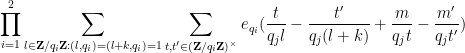
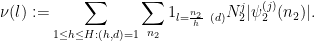
The power savings in Zhang’s Type III argument come from good estimates on the three-dimensional exponential sum

$\displaystyle T(k; m,m'; q) := \sum_{l \in {\bf Z}/q{\bf Z}: (l,q)=(l+k,q)=1} \sum_{t \in ({\bf Z}/q{\bf Z})^\times} \sum_{t' \in ({\bf Z}/q{\bf Z})^\times} \ \ \ \ \ (5)$

$\displaystyle e_q( \frac{t}{l} - \frac{t'}{l+k} + \frac{m}{t} - \frac{m'}{t'} )$

defined for positive integer ${q}$ and ${k,m,m' \in {\bf Z}/q{\bf Z}}$ (or ${k,m,m' \in {\bf Z}}$ ). The key estimate is

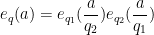
Theorem 4 (Bombieri-Birch bound) Let ${q}$ be square-free. Then for any ${k,m,m' \in {\bf Z}/q{\bf Z}}$ we have

$\displaystyle |T(k; m,m';q)| \ll \frac{(m-m',k,q)}{(k,q)^{1/2}} q^{3/2+o(1)}$

where ${(m-m',k,q)}$ is the greatest common divisor of ${m-m', k, q}$ (and we adopt the convention that ${(0,q)=q}$ ). (Here, the ${o(1)}$ denotes a quantity that goes to zero as ${q \rightarrow \infty}$ , rather than as ${x \rightarrow \infty}$ .)

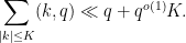
Note that the square root cancellation heuristic predicts ${q^{3/2}}$ as the size for ${T(k;m,m',q)}$ , thus we can achieve better than square root cancellation if ${k}$ has a common factor with ${q}$ that is not shared with ${m-m'}$ . This improvement over the square root heuristic, which is ultimately due to the presence of a Ramanujan sum inside this three-dimensional exponential sum in certain degenerate cases, is crucial to Zhang’s argument.

Proof: Suppose that ${q}$ factors as ${q=q_1q_2}$ , thus ${q_1,q_2}$ are coprime. Then we have

$\displaystyle e_q(a) = e_{q_1}( \frac{a}{q_2} ) e_{q_2} (\frac{a}{q_1})$

(see Lemma 7 of this previous post). From this and the Chinese remainder theorem we see that ${T(k;m,m';q)}$ factorises as

$\displaystyle \prod_{i=1}^2 \sum_{l \in {\bf Z}/q_i{\bf Z}: (l,q_i)=(l+k,q_i)=1} \sum_{t,t' \in ({\bf Z}/q_i{\bf Z})^\times} e_{q_i}( \frac{t}{q_jl} - \frac{t'}{q_j(l+k)} + \frac{m}{q_jt} - \frac{m'}{q_jt'} )$

where ${j := 3-i}$ . Dilating ${t,t'}$ by ${q_j}$ , we conclude the multiplicative law

$\displaystyle T(k;m,m';q_1q_2) = T(k;\frac{m}{q_2^2},\frac{m'}{q_2^2};q_1) T(k;\frac{m}{q_1^2},\frac{m'}{q_1^2};q_2).$

Iterating this law, we see that to prove Theorem 4 it suffices to do so in the case when ${q}$ is prime, or more precisely that

$\displaystyle |T(k; m,m';p)| \ll \frac{(m-m',k,p)}{(k,p)^{1/2}} p^{3/2}.$

We first consider the case when ${k = 0\ (p)}$ , so our objective is now to show that

$\displaystyle |T(0;m,m';p)| \ll (m-m',p) p. \ \ \ \ \ (6)$

In this case we can write ${T(0;m,m';p)}$ as

$\displaystyle \sum_{l,t,t' \in ({\bf Z}/p{\bf Z})^\times} e_p( \frac{t}{l} - \frac{t'}{l} + \frac{m}{t} - \frac{m'}{t'} ).$

Making the change of variables ${s := \frac{tt'}{l}\ (p)}$ , ${u := \frac{1}{t}\ (p)}$ , ${u' := \frac{1}{t'}\ (p)}$ this becomes

$\displaystyle \sum_{s,u,u' \in ({\bf Z}/p{\bf Z})^\times} e_p( su' - su + mu - m' u' ).$

Performing the ${u,u'}$ sums this becomes

$\displaystyle \sum_{s \in ({\bf Z}/p{\bf Z})^\times} C_p(m-s) C_p(s-m')$

where ${C_q(a)}$ is the Ramanujan sum

$\displaystyle C_q(a) := \sum_{b \in ({\bf Z}/q{\bf Z})^\times} e_q(ab).$

Basic Fourier analysis tells us that ${C_p(a)}$ equals ${-1}$ when ${a \neq 0\ (p)}$ and ${p-1}$ when ${a = 0\ (p)}$ . The expression (6) then follows from direct computation.

Next, suppose that ${k \neq 0\ (p)}$ and ${m' = 0\ (p)}$ . Making the change of variables ${s := -\frac{t'}{l+k}}$ , ${T(k;m,0;p)}$ becomes

$\displaystyle \sum_{l \in {\bf Z}/p{\bf Z}: (l,p)=(l+k,p)=1} \sum_{t \in ({\bf Z}/p{\bf Z})^\times} \sum_{s \in ({\bf Z}/p{\bf Z})^\times} e_p( \frac{t}{l} + s + \frac{m}{t} ).$

Performing the ${s}$ summation, this becomes

$\displaystyle - \sum_{l \in {\bf Z}/p{\bf Z}: (l,p)=(l+k,p)=1} \sum_{t \in ({\bf Z}/p{\bf Z})^\times} e_p( \frac{t}{l} + \frac{m}{t} ).$

For each ${l}$ , the ${t}$ summation is a Kloosterman sum and is thus ${O(p^{1/2})}$ by the classical Weil bound (Theorem 8 from previous notes). This gives a net estimate of ${O(p^{3/2})}$ as desired. Similarly if ${m = 0\ (p)}$ .

The only remaining case is when ${k,m,m' \neq 0\ (p)}$ . Here one cannot proceed purely through Ramanujan and Weil bounds, and we need to invoke the deep result of Bombieri and Birch, proven in Theorem 1 of the the appendix to this paper of Friedlander and Iwaniec. This bound can be proven by applying Deligne’s proof of the Weil conjectures to a certain ${L}$ -function attached to the surface ${\{ (x_1,x_2,x_3,x_4): \frac{1}{x_1x_2} + \frac{1}{x_3x_4} = 1 \}}$ ; an elementary but somewhat lengthy second proof is also given in the above appendix. $\Box$

To deal with factors such as ${(k,q)}$ , the following simple lemma will be useful.

Lemma 5 For any ${q}$ and any ${K \geq 1}$ we have

$\displaystyle \sum_{1 \leq k \leq K} (k,q) \ll q^{o(1)} K.$

in particular

$\displaystyle \sum_{t \in {\bf Z}/q{\bf Z}} (t,q) \ll q^{1+o(1)}.$

As in the previous theorem, ${o(1)}$ here denotes a quantity that goes to zero as ${q \rightarrow \infty}$ , rather than as ${x \rightarrow \infty}$ .

Note that it is important that the ${k=0}$ term is excluded from the first sum, otherwise one acquires an additional ${q}$ term. In particular,

$\displaystyle \sum_{|k| \leq K} (k,q) \ll q + q^{o(1)} K.$

Proof: Estimating

$\displaystyle (k,q) \leq \sum_{d|q; d|k} d$

we can bound

$\displaystyle \sum_{1 \leq k \leq K}(k,q) \leq \sum_{d|q} \sum_{1 \leq k \leq K: d|k} d$

$\displaystyle \leq \sum_{d|q} \frac{K}{d} d$

$\displaystyle = K \tau(q)$

$\displaystyle \ll q^{o(1)} K.$

$\Box$

— 2. Cauchy-Schwarz —

We now prove Theorem 3. The reader may wish to track the exponents involved in the model regime

$\displaystyle \delta \approx 0; \quad N_1=N_2=N_3 = N; \quad N \ll d \ll N^{13/8} \ \ \ \ \ (7)$

where ${N}$ is any fixed power of ${x}$ (e.g. ${N = x^{5/16}}$ , in which case ${d}$ can be slightly larger than ${x^{1/2}}$ ).

Let ${\delta,N_1,N_2,N_3,q,\psi_1,\psi_2,\psi_3,a}$ be as in Theorem 3, and let ${\epsilon>0}$ be a sufficiently small fixed quantity. It will suffice to show that

$\displaystyle \sum_{n = a\ (d)} \psi_1 \ast \psi_2 \ast \psi_3(n) = X + O( x^{-\epsilon} \frac{N_1 N_2 N_3}{d} )$

where ${X}$ does not depend on ${a}$ . We rewrite the left-hand side as

$\displaystyle \sum_{n_1} \psi_1(n_1) \sum_{n: (n,q)=1; n_1 = \frac{a}{n}\ (d)} \psi_2 \ast \psi_3(n)$

and then apply completion of sums (Lemma 6 from this previous post) to rewrite this expression as the sum of the main term

$\displaystyle \frac{1}{d} (\sum_{n_1} \psi_1(n_1)) (\sum_{n: (n,d)=1} \psi_2 \ast \psi_3(n))$

plus the error terms

$\displaystyle O( (\log^{O(1)} x) \frac{N_1}{d} \sum_{1 \leq h \le H} |\sum_{n: (n,d)=1} \psi_2 \ast \psi_3(n) e_d( \frac{ah}{n} )| )$

and

$\displaystyle O( x^{-A} \sum_n |\psi_2 \ast \psi_3(n)| ).$

where ${A > 0}$ is any fixed quantity and

$\displaystyle H := x^\epsilon \frac{d}{N_1}.$

The first term does not depend on ${a}$ , and the third term is clearly acceptable, so it suffices to show that

$\displaystyle \sum_{1 \leq h \le H} |\sum_{n: (n,d)=1} \psi_2 \ast \psi_3(n) e_d( \frac{ah}{n} ) | \ll x^{-\epsilon} N_2 N_3. \ \ \ \ \ (8)$

It will be convenient to reduce to the case when ${h}$ and ${d}$ are coprime. More precisely, it will suffice to prove the following claim:

Proposition 6 Let ${\delta>0}$ be fixed, and let

$\displaystyle H, N_2, N_3, d, B \gg 1 \ \ \ \ \ (9)$

be such that

$\displaystyle d \in {\mathcal S}_{[1,x^\delta]}$

and

$\displaystyle H \ll x^{\epsilon} \frac{d}{N_2} \ \ \ \ \ (10)$

and

$\displaystyle N_2^4 N_3^5 \gg B^{-6} d^4 H^4 x^{\delta+c} \ \ \ \ \ (11)$

for some fixed ${c>0}$ , and let ${\psi_2,\psi_3}$ be smooth coefficient sequences at scale ${N_2,N_3}$ respectively. Then

$\displaystyle \sum_{1 \leq h \le H: (h,d)=1} |\sum_{n: (n,d)=1} \psi_2 \ast \psi_3(n) e_d( \frac{ah}{n} ) | \ll x^{-\epsilon} B N_2 N_3$

for some fixed ${\epsilon>0}$ .

Let us now see why the above proposition implies (8). To prove (8), we may of course assume ${H \geq 1}$ as the claim is trivial otherwise. We can split

$\displaystyle \sum_{1 \leq h \leq H} F(h) = \sum_{d = d_1 d_2} \sum_{1 \leq h' \leq H/d_2: (h',d_1)=1} F( d_2 h )$

for any function ${F(h)}$ of ${h}$ , so that (8) can be written as

$\displaystyle \sum_{d = d_1 d_2} \sum_{1 \leq h' \leq H/d_2: (h,d_1)=1} |\sum_{n: (n,d_1 d_2)=1} \psi_2 \ast \psi_3(n) e_{d_1}( \frac{ah'}{n} )|$

which we expand as

$\displaystyle \sum_{d = d_1 d_2} \sum_{1 \leq h' \leq H/d_2: (h,d_1)=1} |\sum_{n_2: (n_2,d_1 d_2)=1} \sum_{n_3: (n_3,d_1d_2)=1} \psi_2(n_2) \psi_3(n_3) e_{d_1}( \frac{ah'}{n_2 n_3} )|$

In order to apply Proposition (6) we need to modify the ${(n_2,d_1d_2)=1}$ , ${(n_3,d_1d_2)=1}$ constraints. By Möbius inversion one has

$\displaystyle \sum_{n_2: (n_2,d_1d_2)=1} F(n_2) = \sum_{b_2|d_2} \mu(b_2) \sum_{n_2: (n_2,d_1)=1} F(b_2 n_2)$

for any function ${F}$ , and similarly for ${n_3}$ , so by the triangle inequality we may bound the previous expression by

$\displaystyle \sum_{d = d_1 d_2} \sum_{b_2|d_2} \sum_{b_3|d_3} F( d_1, d_2, b_1, b_2 ) \ \ \ \ \ (12)$

where

$\displaystyle F(d_1,d_2,b_1,b_2) := \sum_{1 \leq h' \leq H/d_2: (h,d_1)=1}$

$\displaystyle |\sum_{n_2: (n_2,d_1)=1} \sum_{n_3: (n_3,d_1)=1} \psi_2(b_2n_2) \psi_3(b_3n_3)$

$\displaystyle e_{d_1}( \frac{ah'}{b_2b_3 n_2 n_3} )|$

We may discard those values of ${d_2}$ for which ${H' := H/d_2}$ is less than one, as the summation is vacuous in that case. We then apply Proposition (6) with ${d,N_2,N_3,H}$ replaced by ${d_1,N_2/b_2,N_3/b_3,H'}$ respectively and ${B}$ set equal to ${b_2 b_3}$ , and ${\psi_2,\psi_3}$ replaced by ${\psi_2(b_2\cdot)}$ and ${\psi_3(b_3\cdot)}$ . One can check that all the hypotheses of Proposition 6 are obeyed, so we may bound (12) by

$\displaystyle \ll x^{-\epsilon} N_2 N_3 \sum_{d = d_1 d_2} \sum_{b_2|d_2} \sum_{b_3|d_3} 1$

which by the divisor bound is ${\ll x^{-\epsilon+o(1)} N_2 N_3}$ , which is acceptable (after shrinking ${\epsilon}$ slightly).

It remains to prove Proposition 6. Continuing (7), the reader may wish to keep in mind the model case

$\displaystyle \delta \approx 0; N_2 = N_3 = N; \quad N \ll d \ll N^{13/8}; \quad H \approx d/N; \quad B \approx 1.$

Note from (9), (10) one has

$\displaystyle d \gg x^{-\epsilon} N_2. \ \ \ \ \ (13)$

Expanding out the ${\psi_2 \ast \psi_3}$ convolution, our task is to show that

$\displaystyle \sum_{1 \leq h \le H: (h,d)=1} |\sum_{n_2: (n_2,d)=1} \sum_{n_3: (n_3,d)=1} \psi_2(n_2) \psi_3(n_3) e_d( \frac{ah}{n_2n_3} )| \ll x^{-\epsilon} B N_2 N_3. \ \ \ \ \ (14)$

As before, our aim is to obtain a power savings better than ${H}$ over the trivial bound of ${H N_2 N_3}$ .

The next step is Weyl differencing. We will need a step size ${r \geq 1}$ which we will optimise in later. We set

$\displaystyle K := \lfloor x^{-\epsilon} N_2 r^{-1} H^{-1}\rfloor; \ \ \ \ \ (15)$

we will make the hypothesis that

$\displaystyle K \geq 1 \ \ \ \ \ (16)$

and save this condition to be verified later.

By shifting ${n_2}$ by ${khr}$ for ${1 \leq k \leq K}$ and then averaging, we may write the left-hand side of (14) as

$\displaystyle \sum_{1 \leq h \le H: (h,d)=1} |\frac{1}{K} \sum_{1 \leq k \leq K} \sum_{n_2: (n_2,d)=1} \sum_{n_3: (n_3,d)=1}$

$\displaystyle \psi_2(n_2+hkr) \psi_3(n_3) e_d( \frac{ah}{(n_2+hkr)n_3} )|.$

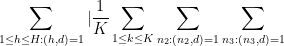
By the triangle inequality, it thus suffices to show that

$\displaystyle \sum_{1 \leq h \leq H: (h,d)=1} \sum_{n_2: (n_2,d)=1} |\sum_{1 \leq k \leq K} \psi_2(n_2+hkr) \ \ \ \ \ (17)$

$\displaystyle \sum_{n_3: (n_3,d)=1} \psi_3(n_3) e_d( \frac{ah}{(n_2+hkr)n_3} )| \ll x^{-\epsilon} B K N_2 N_3.$

Next, we combine the ${h}$ and ${n_2}$ summations into a single summation over ${{\bf Z}/d{\bf Z}}$ . We first use a Taylor expansion and (15) to write

$\displaystyle \psi_2(n_2+hkr) = \sum_{j=0}^J \frac{1}{j!} (h/H)^j N_2^{j} \psi_2^{(j)}(n_2) (Hkr/N_2)^j + O( x^{-J\epsilon+o(1)})$

for any fixed ${J}$ . If ${J}$ is large enough, then the error term will be acceptable, so it suffices to establish (17) with ${\psi_2(n_2+hkr)}$ replaced by ${(h/H)^j N_2^j \psi_2^{(j)}(n_2) (hkr/N_2)^j}$ for any fixed ${j \geq 0}$ . We can rewrite

$\displaystyle e_d( \frac{ah}{(n_2+hkr)n_3} ) = e_d( \frac{a}{(l+kr) n_3} )$

where ${l \in {\bf Z}/d{\bf Z}}$ is such that ${(l+kr,d)=1}$ and

$\displaystyle l = \frac{n_2}{h}\ (d).$

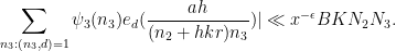
Thus we can estimate the left-hand side of (17) by

$\displaystyle \sum_{l \in {\bf Z}/d{\bf Z}} \nu(l) |\sum_{1 \leq k \leq K: (l+kr,d)=1} (Hkr/N_2)^j \ \ \ \ \ (18)$

$\displaystyle \sum_{n_3: (n_3,d)=1} \psi_3(n_3) e_d( \frac{a}{(l+kr) n_3})|$

where

$\displaystyle \nu(l) := \sum_{1 \leq h \leq H: (h,d)=1} \sum_{n_2} 1_{l = \frac{n_2}{h}\ (d)} N_2^j |\psi_2^{(j)}(n_2)|.$

Here we have bounded ${(h/H)^j}$ by ${O(1)}$ .

We will eliminate the ${\nu}$ expression via Cauchy-Schwarz. Observe from the smoothness of ${\psi_2}$ that

$\displaystyle \nu(l) \ll x^{o(1)} |\{ (h,n_2): 1 \leq h \leq H; 1 \ll n_2 \ll N_2; (h,d)=1; l = \frac{n_2}{h}\ (d) \}|$

and thus

$\displaystyle \sum_l \nu(l)^2 \ll x^{o(1)} |\{ (h,h',n_2,n'_2): 1 \leq h,h' \leq H; 1\ll n_2,n'_2 \ll N_2;$

$\displaystyle (h,d)=(h',d) = 1; \frac{n_2}{h} = \frac{n'_2}{h'}\ (d) \}|.$

Note that ${\frac{n_2}{h} = \frac{n'_2}{h'}\ (d)}$ implies ${n_2 h' = n'_2 h\ (d)}$ . But from (10) we have ${1 \leq n_2 h', n'_2 h \leq d}$ , so in fact we have ${n_2 h' = n'_2 h}$ . Thus

$\displaystyle \sum_l \nu(l)^2 \ll x^{o(1)} |\{ (h,h',n_2,n'_2): 1 \leq h' \leq H; 1\ll n_2 \ll N_2; n_2 h' = n'_2 h \}|.$

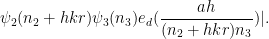
From the divisor bound, we see that for each fixed ${n_2, h'}$ there are ${O(x^{o(1)})}$ choices for ${n'_2,h}$ , thus

$\displaystyle \sum_l \nu(l)^2 \ll x^{o(1)} N_2 H.$

From this, (18), and Cauchy-Schwarz, we see that to prove (17) it will suffice to show that

$\displaystyle \sum_{l \in {\bf Z}/d{\bf Z}} |\sum_{1 \leq k \leq K: (l+kr,d)=1} (Hkr/N_2)^j \ \ \ \ \ (19)$

$\displaystyle \sum_{n_3: (n_3,d)=1} \psi_3(n_3) e_d( \frac{a}{(l+kr) n_3})|^2$

$\displaystyle \ll x^{-2\epsilon} B^{2} K^2 N_2 N_3^2 H^{-1}.$

Comparing with the trivial bound of ${O( d N_3^2 K^2 )}$ , our task is now to gain a factor of more than ${\frac{B^2Hd}{N_2}}$ over the trivial bound.

We square out (19) as

$\displaystyle \sum_{1 \leq k,k' \leq K}\sum_{l \in {\bf Z}/d{\bf Z}: (l+kr,d)=(l+k'r,d)=1} (Hkr/N_2)^j (Hk'r/N_2)^j$

$\displaystyle \sum_{n_3,n'_3: (n_3,d)=(n'_3,d)=1} \psi_3(n_3) \overline{\psi_3}(n_3) e_d( \frac{a}{(l+kr)n_3)} - \frac{a}{(l+k'r)n'_3} ).$

If we shift ${l}$ by ${kr}$ , then relabel ${k'-k}$ by ${k}$ , and use the fact that ${Hkr/N_2, Hk'r/N_2 = O(1)}$ , we can reduce this to

$\displaystyle \sum_{|k| \leq K}$

$\displaystyle |\sum_{l \in {\bf Z}/d{\bf Z}: (l,d)=(l+kr,d)=1} \sum_{n_3,n'_3: (n_3,d)=(n'_3,d)=1}$

$\displaystyle \psi_3(n_3) \overline{\psi_3}(n_3) e_d( \frac{a}{ln_3} - \frac{a}{(l+kr)n'_3} )|$

$\displaystyle \ll x^{-2\epsilon} B^{2} K N_2 N_3^2 H^{-1}.$

Next we perform another completion of sums, this time in the ${n_3,n'_3}$ variables, to bound

$\displaystyle |\sum_{l \in {\bf Z}/d{\bf Z}: (l,d)=(l+kr,d)=1} \sum_{n_3,n'_3: (n_3,d)=(n'_3,d)=1}$

$\displaystyle \psi_3(n_3) \overline{\psi_3}(n_3) e_d( \frac{a}{ln_3} - \frac{a}{(l+kr)n'_3} )|$

$\displaystyle \ll x^{o(1)} \sum_{|m|, |m'| \leq M'} (\frac{N_3}{d})^2 | U(k; m,m'; d)|+ x^{-A}$

for any fixed ${A>0}$ , where

$\displaystyle M' := x^{\epsilon} \frac{d}{N_3} \ \ \ \ \ (20)$

(the prime is there to distinguish this quantity from ${M}$ in the introduction) and

$\displaystyle U(k;m,m';d) := \sum_{l \in {\bf Z}/d{\bf Z}: (l,d)=(l+kr,d)=1} \sum_{n_3,n'_3 \in ({\bf Z}/d{\bf Z})^\times}$

$\displaystyle e_d( \frac{a}{ln_3} - \frac{a}{(l+kr)n'_3} + mn_3 - m' n'_3).$

Making the change of variables ${t := \frac{a}{n_3}\ (d)}$ and ${t' := \frac{a}{n'_3}\ (d)}$ and comparing with(5), we see that

$\displaystyle U(k;m,m';d) = T( kr; am, am'; d).$

Applying Theorem 4 (and recalling that ${a \in ({\bf Z}/d{\bf Z})^\times}$ ) we reduce to showing that

$\displaystyle \sum_{|k| \leq K} \sum_{|m|, |m'| \leq M'} \frac{(kr,m-m',d)}{(kr,d)^{1/2}} (\frac{N_3}{d})^2 d^{3/2} \ll x^{-3\epsilon} B^{2} K N_2 N_3^2 H^{-1}.$

We now choose ${r}$ to be a factor of ${d}$ , thus

$\displaystyle d = qr$

for some ${q}$ coprime to ${r}$ . We compute the sum on the left-hand side:

Lemma 7 We have

$\displaystyle \sum_{|k| \leq K} \sum_{|m|, |m'| \leq M'} \frac{(kr,m-m',d)}{(kr,d)^{1/2}}$

$\displaystyle \ll x^{o(1)} ( M' r^{1/2} K + M' d^{1/2} + (M')^2 K r^{-1/2} ).$

Proof: We first consider the contribution of the diagonal case ${m=m'}$ . This term may be estimated by

$\displaystyle \ll M' \sum_{|k| \leq K} (kr,d)^{1/2} = M' r^{1/2} \sum_{|k| \leq K} (k,q)^{1/2}.$

The ${k=0}$ term gives ${M'd^{1/2}}$ , while the contribution of the non-zero ${k}$ are acceptable by Lemma 5.

For the non-diagonal case ${m \neq m'}$ , we see from Lemma 5 that

$\displaystyle \sum_{|m|,|m'| \leq M': m \neq m'} (kr,m-m',d) \ll x^{o(1)} (M')^2;$

since ${(kr,d) \geq r}$ , we obtain a bound of ${O( x^{o(1)} (M')^2 K r^{-1/2} )}$ from this case as required. $\Box$

From this lemma, we see that we are done if we can find ${r}$ obeying

$\displaystyle (M' r^{1/2} K + M' d^{1/2} + (M')^2 K r^{-1/2} ) (\frac{N_3}{d})^2 d^{3/2} \ll x^{-4\epsilon} B^{2} K N_2 N_3^2 H^{-1}. \ \ \ \ \ (21)$

as well as the previously recorded condition (16). We can split the condition (21) into three subconditions:

$\displaystyle M' r^{1/2} d^{-1/2} \ll x^{-4\epsilon} B^{2} N_2 H^{-1}$

$\displaystyle M' K^{-1} \ll x^{-4\epsilon} B^{2} N_2 H^{-1}$

$\displaystyle (M')^2 r^{-1/2} d^{-1/2} \ll x^{-4\epsilon} B^{2} N_2 H^{-1}.$

Substituting the definitions (15), (20) of ${K, M'}$ , we can rewrite all of these conditions as lower and upper bounds on ${r}$ . Indeed, (16) follows from (say)

$\displaystyle r \ll n^{-2\epsilon} N_2 H^{-1} \ \ \ \ \ (22)$

while the other three conditions rearrange to

$\displaystyle r \ll x^{-10\epsilon} B^{4} N_2^2 N_3^2 H^{-2} d^{-1} \ \ \ \ \ (23)$

$\displaystyle r \ll x^{-6\epsilon} B^{2} N_2^2 N_3 H^{-2} d^{-1} \ \ \ \ \ (24)$

and

$\displaystyle r \gg x^{12\epsilon} B^{-4} N_2^{-2} N_3^{-4} H^2 d^{3}.$

We can combine (23), (24) into a single condition

$\displaystyle r \ll x^{-10\epsilon} B^{2} N_2^2 N_3 H^{-2} d^{-1}.$

Also, from (9), (13) we see that this new condition also implies (22). Thus we are done as soon as we find a factor ${r}$ of ${d}$ such that

$\displaystyle R_1 \ll r \ll R_2$

where

$\displaystyle R_1 := x^{12\epsilon} B^{2} N_2^{-2} N_3^{-4} H^2 d^{3}$

and

$\displaystyle R_2 := x^{-6\epsilon} B^{-4} N_2^2 N_3 H^{-2} d^{-1}.$

From (11) one has

$\displaystyle R_2/R_1 \gg x^\delta$

if ${\epsilon}$ is sufficiently small. Also, from (11), (9) one also sees that

$\displaystyle R_1 \ll d$

and ${R_2 \gg 1}$ . As ${d}$ is ${x^\delta}$ -smooth, we can thus find ${r}$ with the desired properties by the greedy algorithm. (In view of Corollary 12 from this previous post, one could also have ensured that ${q}$ has no tiny factors, although this does not seem to be of much actual use in the Type III analysis.)

83 comments

Comments feed for this article

14 June, 2013 at 9:38 am

Terence Tao

While writing up the argument I found that the factorisation of the Bombieri-Birch exponential sum for a mdulus d=qr into a modulus q component (which is still of Bombieri-Birch type) and a modulus r component (which is of Ramanujan type) could be more cleanly performed by noting a multiplicativity property of the Bombieri-Birch sum (see the third display in the proof of Theorem 4). This in particular leads to a refinement of Lemma 12 of Zhang that “bakes in” the Ramanujan sum decay more efficiently. This ended up cleaning up the proof (as did application of completion of sums as a black box estimate, without any further need to track Fourier coefficients) but unfortunately did not lead to improved bounds.

As before, we can record the numerics of the critical case:

$\varpi = 1/899 \approx 0.00111$

$\delta = 71/154628 \approx 0.000460$

$N_1=N_2=N_3 = N\approx x^{47795/154628} \approx x^{0.309097}$

$M \approx x/N^3 \approx x^{0.072710}$

$d \approx x^{1/2+2\varpi} \approx x^{0.502245} \approx N^{1.62481}$

$x^\delta \approx N^{0.001486}$

$M', H \approx d/N \approx N^{0.62481}$

$R_1 \approx N^{0.124072}$

$R_2 \approx N^{0.125557}$

$R_1 \ll r \ll R_2$

$K \approx N/Hr \approx N^{0.387952}/r$

14 June, 2013 at 2:13 pm

bengreen

This multiplicativity property is a nice observation. It reduces some of the mystery.

16 June, 2013 at 3:01 am

v08ltu

There is something wrong in the above. I get that $K$ is less than 1. Its exponent is $0.387952\times0.309097-0.124\ldots<0$ .

16 June, 2013 at 3:02 am

v08ltu

Oh, duh I mixed N and x, sorry!

14 June, 2013 at 10:03 am

Terence Tao

Three thoughts:

1. The triple exponential sum in Theorem 4 has the unusual property that certain degenerate cases of this sum are smaller than the non-degenerate cases (in particular, beating square root cancellation) – usually the degenerate cases are much larger. This leads to certain “diagonal” terms in the Cauchy-Schwarz analysis being significantly smaller than what one would naively expect them to be. The rarity of this phenomenon (degenerate sums being better behaved than non-degenerate sums) may limit the applicability of this very nice trick of Zhang.

2. Zhang’s trick should improve the numerical values of the recent preprint of Fouvry, Kowalski, and Iwaniec http://arxiv.org/abs/1304.3199 on the level of distribution of $\tau_3$ , at least when restricted to smooth moduli. But this is outside the scope of the polymath project and I would presume that FKM are already in the process of working out the details, so I propose that we avoid pursuing this direction here. (But it might be worth leafing through FKM to see if there are any tricks that can also be applied to the Type III sums here.)

3. The discarding of the $\alpha$ convolution to reduce Theorem 2 to Theorem 3 looks lossy. In particular it seems to me that Theorem 2 only requires an averaged version of Theorem 3 in which the $a$ parameter is averaged over a set of length M (the inverse of an arithmetic progression in ${\bf Z}/d{\bf Z}$ ). I have a suspicion that completion of sums is less lossy when there is such an averaging, in principle one might gain an additional factor of something like $M^{1/2}$ . This could lead to some noticeable numerical improvements in the exponents. However, I have not yet worked out the details of this.

14 June, 2013 at 2:27 pm

v08ltu

Regarding #1, I too thought this mysterious. I mean, so you Weyl shift by multiples of $r$ – why doesn’t that just give you something like $e_r(0)$ (and thus no cancellation) rather than a Ramanujan sum (with residue-class differences as an argument)? This is still a philosophy disparity for me.

14 June, 2013 at 9:24 pm

Terence Tao

Actually, now that I think about it, I know another context in which partly degenerate exponential sums have better cancellation than non-degenerate sums. Consider a quadratic exponential sum $\sum_{n \in {\bf Z}/p{\bf Z}} e_p( an^2 + bn)$ for some odd prime $p$ . When $a$ is non-zero this is a Gauss sum and has square root cancellation – the magnitude is exactly $\sqrt{p}$ . But when $a$ degenerates to zero while $b$ stays non-zero, we get perfect cancellation – the magnitude is now zero! Of course, when $a$ and $b$ both degenerate, there is no cancellation whatsoever and the sum jumps up to $p$ .

With the Birch-Bombieri sum $\sum_{l \in {\bf Z}/q{\bf Z}: (l,q)=(l+k,q)=1} \sum_{t,t' \in ({\bf Z}/q{\bf Z})^\times} e_q( \frac{t}{l} - \frac{t'}{l+k} + \frac{m}{t} - \frac{m'}{t'} )$ there is a qualitatively similar phenomenon: square root cancellation in the fully non-degenerate case, better than square root cancellation in the partially degenerate case ( $k$ has a common factor with $q$ but $m-m'$ does not), and huge in the completely degenerate case.

17 June, 2013 at 12:13 am

Emmanuel Kowalski

FKI should be FKM…. (Fouvry-K.-Michel)

[Corrected, thanks – T.]

18 June, 2013 at 6:08 am

Ph.M

Regarding # 2.
In fact, when an averaging over conveniently factorable moduli is available (as in this case here) we checked is it possible to get a quite high exponent of distribution (up to 4/7). The argument is simpler than Zhang’s treatment and in fact should improve Zhang type III sums quite a bit. See one of Emmanuel’s forth coming blog.

19 June, 2013 at 1:15 am

v08ltu

If I take this comment in the most direct sense, we have $4/7=1/2+2\omega$ when $\omega=1/28$ . With no $\kappa$ or $\delta$ this would give $k_0=110$ , but perhaps other aspects will break.

19 June, 2013 at 4:49 am

Andrew Sutherland

We would then have H(110)=628 (from Engelsma’s tables).

19 June, 2013 at 6:47 am

Terence Tao

If the Type III sums became that good then the bottleneck then comes from the Type I/II sums (which currently has a constraint of the form $37 \varpi + 5\delta < \frac{1}{4}$ ) and also the combinatorial analysis (which has a constraint $\sigma > 1/10$ , which when combined with the constraint $11\varpi + 3\delta+ 2\sigma < \frac{1}{4}$ coming from the Type I analysis gives that $11 \varpi + 3 \delta < \frac{1}{20}$ ). The second barrier is a bit stronger, so there is a barrier to $\varpi$ getting past $1/220$ at present, but we have basically made no efforts to attack these barriers yet as they have not come close to the battlefront thus far, and presumably they can be knocked back a bit. But in any event I foresee that the Type III sums will cease to become critical in the near future, and we will have to turn our attention elsewhere to get gains.

19 June, 2013 at 7:18 am

Ph.M

Actually, the exponent $4/7$ is for the distribution of $d_3$ which is “smoother” than the actual type III which includes some small non smooth factor ( the variable $m\sim M$ ) so the $4/7$ exponent is relative to $x/M$ rather than $x$ . We will write this up.

19 June, 2013 at 7:56 am

Terence Tao

Naively, if one assumes a $4/7$ level of distribution for the $d_3$ component of the type III sums, one expects a condition of the form

$x^{1/2 + 2 \varpi} \ll (N_1 N_2 N_3)^{4/7}$

(ignoring epsilons) which on plugging in the critical case $N_1=N_2=N_3 = x^{(1/2+\sigma)/2}$ from the combinatorial analysis gives

$\frac{1}{2} + 2 \varpi < \frac{4}{7} \frac{3}{2} (\frac{1}{2} + \sigma )$

thus

$\sigma > \frac{1}{12} + \frac{7}{3} \varpi$ .

From Type I analysis (and ignoring $\delta$ and infinitesimals) we can take $\sigma = 1/8 - 11 \varpi/2$ so this gives a constraint $\varpi < 1/188$ , but this is unfortunately occluded by the existing constraint $\varpi < 1/220$ coming from the requirement $\sigma > 1/10$ . It may well be that one can also exploit the $\alpha$ averaging as we are currently doing but this will only serve to weaken the $\varpi < 1/188$ threshold and not the $\varpi < 1/220$ one. So my prediction is that the Type III improvement will be strong enough that it no longer provides the dominant obstruction to bounds, with the combinatorial constraint $\sigma > 1/10$ (combined with the constraint $11 \varpi + 2 \sigma < 1/4$ from the Type I analysis) dominating instead, and basically placing $\varpi$ close to $1/220$ .

14 June, 2013 at 12:51 pm

Pace Nielsen

“Chiense” should be “Chinese”

In equation (8) there is an extra left-hand absolute value sign. [It might be more readable to make some of the absolute value signs bigger, so it is clear they encompass some of the sums.]

In the third offset equation above (8), it appears that a right-hand absolute value sign is missing.

Sorry for not having any useful things to say about the mathematics. I am enjoying reading these posts.

[Corrected, thanks – T.]

14 June, 2013 at 1:40 pm

Pace Nielsen

I did have one question, about the definition of “coefficient sequence”. Isn’t every finitely supported sequence a coefficient sequence? From the finite support, we know that the image of the sequence is bounded. But for sufficiently large x, log(x) then dominates. (Or is x not independent of n and $\alpha$ somehow?)

14 June, 2013 at 2:42 pm

v08ltu

I had the same fret, reading this definition before. It’s finitely supported, but has some asymptotic bounds? I guess this needs to be interpreted, as saying that the constants in the $\ll$ have been picked before hand?

14 June, 2013 at 5:55 pm

Terence Tao

Every fixed (i.e. independent of x) finitely supported sequence is a coefficient sequence, but a finitely supported sequence that depends on x need not be a coefficient sequence. (The distinction between quantities that depend on the asymptotic parameter $x$ , and quantities independent of that parameter (which are called “fixed”) here, forms the basis of what I call “cheap nonstandard analysis“, which allows one to work rigorously with asymptotic notation without having to deploy the full machinery of nonstandard analysis. It is briefly introduced in the earliest of this series of posts, back at https://terrytao.wordpress.com/2013/06/03/the-prime-tuples-conjecture-sieve-theory-and-the-work-of-goldston-pintz-yildirim-motohashi-pintz-and-zhang/ .

15 June, 2013 at 12:07 pm

Gaston Rachlou

In my humble opinion, this terminology is not a very happy innovation, and could be replaced with no harm by its definition, accessible to any mathematician. One has to understand that your $\alpha(n)$ is in fact a $\alpha(n,x)$ . Moreover, it is not immediately clear if the support of this sequence (supposed to be finite for $x$ fixed) depends on $x$ or not.

15 June, 2013 at 12:51 pm

Terence Tao

To quote from the first post in this series where this notation is introduced:

“Some mathematical objects (such as ${\mathcal H}$ and $k$ ) will be independent of $x$ and referred to as fixed; but unless otherwise specified we allow all mathematical objects under consideration to depend on $x$ .”

The alternative would be to explicitly subscript almost every quantity (other than the fixed ones) in these posts by $x$ , which would be quite distracting, since this dependence occurs for most of the objects introduced in the post and thus is better suited to be the default assumption in one’s notation as specified above, rather than the other way around. (For instance, in the above post, the objects $\alpha, \beta, \nu, \psi, \psi_1, \psi_2, \psi_3, a, b, b_1, b_2, d, d_1, d_2, k, l, m, m', n$ , $n_1, n_2, n_3, p, q, r, t, t', x$ , $F, I, H, K, M, N$ , $N_1, N_2, N_3$ , $R_1, R_2, X, Y$ and associated structures (e.g. the support of $\alpha$ ) are allowed to depend on $x$ or to be bound to a range depending on $x$ (as indicated by the default convention that is in force throughout these posts), with only $\delta, \varepsilon, \varpi, c, i, j, A, A_0$ declared as fixed.)

15 June, 2013 at 8:39 am

meditationatae

The Bombieri-Birch bound in Theorem 4 is given in long outline form above, although presumably this wasn’t re-argued in Zhang’s paper, am I right? In expression (6), it seems that $p$ is the same thing as the $q$ assumed prime about four lines above, in the “case when $q$ is prime” . It seems Zhang’s proof of Theorem 3 involves invoking the Bombieri-Birch triple exponential sum bound of Theorem 4, and all that lies in Section 2 of the post, starting at expression (7) till the end of Section 2; is that about right? Finally, my intuition is that Theorem 2 is not so hard, given Theorem 3, and the “hard theorem” would be Theorem 3, Zhang’s Type III estimate without $\alpha$ …

15 June, 2013 at 9:22 am

Terence Tao

Yes, this is basically correct. Theorem 4 above corresponds to Lemma 11 in Zhang, although Theorem 4 is also recording an additional cancellation in the degenerate case when k has a shared factor with q but not m-m’; this cancellation was implicit in Section 14 but it seems simpler to place it in Theorem 4 instead.

15 June, 2013 at 1:47 pm

Terence Tao

I think I can indeed get some gain here from working with an averaged version of Theorem 3. More precisely, if one inspects the derivation of Theorem 2 from Theorem 3, we see that it actually suffices to replace the conclusion of Theorem 3 by the weaker

$|{\bf E}_{a \in A} c_a \Delta(\psi_1 \ast \psi_2 \ast \psi_3; a)| \ll x^{-\varepsilon} \frac{N_1 N_2 N_3}{d}$

where $A := \{ a_0/m: M \ll m \ll M \} \subset ({\bf Z}/d{\bf Z})^\times$ for some $a_0 \in ({\bf Z}/d{\bf Z})^\times$ and the coefficients $c_a$ are $O(1)$ . (In the regime of interest we have $M \ll d$ .)

If we run the arguments of Section 2 carrying this new averaging in A with us, (8) becomes

$\sum_{1 \leq h \leq H} | {\bf E}_{a \in A} c_a \sum_{n: (n,d)=1} \psi_2 \ast \psi_3(n) e_d(\frac{ah}{n})| \ll x^{-\varepsilon} N_2 N_3$

and the conclusion of Proposition 6 is similarly replaced with

$\sum_{1 \leq h \leq H: (h,d)=1} | {\bf E}_{a \in A} c_a \sum_{n: (n,d)=1} \psi_2 \ast \psi_3(n) e_d(\frac{ah}{n})| \ll x^{-\varepsilon} N_2 N_3$ .

Continuing the argument through to (19), we see that (19) is replaced with

$\sum_{l \in {\bf Z}/d{\bf Z}} | \sum_{1 \leq k \leq K: (l+kr,d)=1}$

${\bf E}_{a \in A} c_a \sum_{n_3: (n_3,d)=1} \psi_3(n_3) e_d(\frac{a}{(l+kr)n_3})|^2$

$\ll x^{-2\varepsilon} K^2 N_2 N_3^2 H^{-1}$

Squaring this out and continuing the arguments of the main post, we see that it suffices to establish the bound

$\sum_{|k| \leq K} \sum_{|m|, |m'| \leq M'} {\bf E}_{a,a' \in A} (\frac{N_3}{d})^2|T(kr; am, a'm'; d)|$

$\ll x^{-3\varepsilon} K N_2 N_3^2 H^{-1};$

note crucially that the third argument of the exponential sum $T$ now acquires a factor of a’ instead of a. Using Theorem 4, the left-hand side is essentially bounded by

$\sum_{|k| \leq K} \sum_{|m|, |m'| \leq M'} {\bf E}_{a,a' \in A} (\frac{N_3}{d})^2$

$\frac{(kr,am-a'm',d)}{(kr,d)^{1/2}}.$

The key point here is that generic $a,a' \in A$ are usually coprime, making the diagonal case $am=am'$ somewhat rarer than the diagonal case $m=m'$ considered in Lemma 7. Writing $a = b/\tilde m$ , $a' = b/\tilde m'$ for $\tilde m, \tilde m' \sim M$ , one can rewrite

$(kr,am-a'm',d) = (kr,\tilde m'm - \tilde m m', d)$

and by using the divisor bound this is basically back to the situation in Lemma 7 but with m, m’ now ranging at scale O(MM’) rather than just O(M’). As such, the first two terms on the RHS of Lemma 7 acquire an additional factor of M^{-1} after performing the averaging in a,a’. According to my calculations, this allows one to loosen the constraint

$N_2^4 N_3^5 \gg d^4 H^4 x^{\delta+c}$

in Proposition 6 with the pair of constraints

$M N_2^4 N_3^5 \gg d^4 H^4 x^{\delta+c}$

$N_2^3 N_3^4 \gg d^3 H^2 x^{\delta+c}$

(the latter condition comes from (22) which is no longer so obviously dominated by (24), although it will ultimately still be redundant in the final analysis after optimising with the Type I/II analysis). This means that we can replace

$N_1^4 N_2^4 N_3^5 \gg x^{4+16\varpi+\delta+c}$

in Theorem 2 with

$M N_1^4 N_2^4 N_3^5 \gg x^{4+16\varpi+\delta+c}$

and

$N_1^2 N_2^3 N_3^4 \gg x^{5/2 + 10\varpi+\delta+c}.$

The former constraint is equivalent to

$N_1^3 N_2^3 N_3^4 \gg x^{3+16\varpi+\delta+c}.$

Returning to the combinatorial analysis, the necessary condition

$\frac{13}{2} (\frac{1}{2}+\sigma) > 4 + 16 \varpi + \delta$

is now relaxed to the combination of

$5 (\frac{1}{2}+\sigma) > 3 + 16 \varpi + \delta$

and

$\frac{9}{2} (\frac{1}{2}+\sigma) > \frac{5}{2} + 10 \varpi + \delta$

which, upon setting $\sigma$ close to $1/8 - 11/2 \varpi - 3/2 \delta$ (and also recalling the condition $\sigma > 1/10$ ) becomes (if all my calculations are correct)

$87 \varpi + 17 \delta < 1/4$

and

$139 \varpi + 13 \delta < 5/4$

and

$11 \varpi + 3 \delta < \frac{1}{20}.$

The second and third conditions are weaker than the first so we are left with $87 \varpi + 17 \delta < 1/4$ , which would be a significant improvement over the previous bound of $207 \varpi + 43 \delta < 1/4$ .

Needless to say, this should all be checked, and should be currently viewed as provisional, but I'm optimistic that we have a good gain here.

15 June, 2013 at 4:04 pm

v08ltu

I have been too busy to be PolyMathing recently, but I think that the work of Ping Xi on Burgess for Kloosterman sums that I mentioned in the other thread has good hope of some improvement on the other end of things. The main technical issue is to pass from prime to composite moduli (and write the details of the proof in the first place) w/o losing too much, which is not always trivial in a Burgess setting (it is not simply CRT) vis-a-vis coprimality accounting.

I contend that the main “problem” with 13&14 was that the diagonal was so dominant (that K needed to be so big), and so your idea seems to quell it via averaging. What is the critical K with these provisional parameters?

15 June, 2013 at 10:55 pm

v08ltu

I agree that this $m$-averaging should in principle work. But to verify all the details I still need to change your notation into my notation (and compare to Zhang’s notation, particularly ensuring that “m” is not confused with “m” any where).

16 June, 2013 at 4:41 am

Michael

I think the redundant inequality near the end should have $31\delta$ instead of $33\delta$

[Corrected, thanks; also I added the additional constraint $\sigma > 1/10$ from the combinatorial analysis. Fortunately, neither of these corrections ended up affecting the headline bound. -T]

15 June, 2013 at 3:59 pm

Andrew Sutherland

Do we know approximately what value this would imply for $k_0$ ?

15 June, 2013 at 4:11 pm

v08ltu

I think $\omega=1/382$ and $k_0=6330$ works, but I have to run.

15 June, 2013 at 6:25 pm

Terence Tao

Here’s what I get with this choice of parameters (ignoring infinitesimals):

$\omega = 1/382 \approx 0.002618$

$k_0 = 6330$

$\delta = 1/764 \approx 0.001309$

and

$\frac{1+4\varpi}{j_{k_0-2}^2 / k_0(k_0-1)} \approx 1.00005395$

which gives us about $5.395 \times 10^{-5}$ of room for $\kappa$ and $\kappa'$ . Using Gergely’s first improved value

$\kappa = \sum_{1 \leq n < \frac{1+4\varpi}{4\delta}} \frac{3^n+1}{2} \frac{k_0^n}{n!} (\int_{4\delta/(1+4\varpi)}^1 (1 - t)^{k_0/2}\ \frac{dt}{t})^n$

$\kappa' = \sum_{2 \leq n < \frac{1+4\varpi}{4\delta}} \frac{3^n-1}{2} \frac{(k_0-1)^n}{n!} (\int_{4\delta/(1+4\varpi)}^1 (1 - t)^{(k_0-1)/2}\ \frac{dt}{t})^n$

of $\kappa,\kappa'$ (the derivation of which is now in the main post of https://terrytao.wordpress.com/2013/06/11/further-analysis-of-the-truncated-gpy-sieve/ ), I get $\kappa \approx 5.25 \times 10^{-5}$ and $\kappa' \approx 1.39 \times 10^{-9}$ , so the bar looks like it is cleared (though I do not have an error analysis on the numerical integration I performed). With Gergely’s provisional values of $\kappa,\kappa'$ I get essentially the same result. So I am happy to confirm the $k_0=6330$ value once the $84\varpi+17\delta < 1/4$ condition is confirmed.

For the above values of $\varpi,\delta$ , we can recalculate the critical numerology as follows:

$\sigma = \frac{1}{8} - \frac{11 \varpi}{2} - \frac{3 \delta}{2} = \frac{83}{764} \approx 0.108639$

$N_1 = N_2 = N_3 = N = x^{(1/2+\sigma)/2} \approx x^{0.304319}$

$M \approx x/N^3 \approx x^{0.08704}$

$d \approx x^{1/2+2\varpi} \approx x^{0.505237}$

$H \approx M' \approx d/N \approx x^{0.200916}$

$x^{0.091623} \ll r \ll x^{0.09293}$

$x^{0.010471} \ll K \ll x^{0.011780}$

So K is looking a lot smaller than it used to be (in the previous critical case, it was closer to $x^{0.26}$ ).

I have to run, but I will try to confirm Gergely’s new provisional argument for $\kappa,\kappa'$ soon (and maybe sneak a look at the Ping Xi paper, though this may have to wait a bit). I’ll also have to double-check the $84\varpi+17\delta < 1/4$ argument, though if someone else could also have a look at this, that would be great.

15 June, 2013 at 6:33 pm

v08ltu

I get $\omega=1/381.6$ allows $k_0=6329$ .

15 June, 2013 at 6:37 pm

v08ltu

In fact, $\omega=1/382$ also allows $k_0=6329$ (just barely), not sure why I missed it the first time around, but I was in a hurry. I will try to sort through the new argument for 13&14. The condition is “87” omega, correct? In the latter comment you twice have “84”. I will work thru it in any case.

15 June, 2013 at 8:06 pm

Terence Tao

Oops, sorry about that, that was a typo and I have just corrected it. Yes, the correct condition (I believe) is $87 \varpi + 17 \delta < \frac{1}{4}$ .

15 June, 2013 at 6:42 pm

Gergely Harcos

Sounds great. For $k_0=6329$ I get $\frac{1+4\varpi}{j_{k_0-2}^2 / k_0(k_0-1)} \approx 1.00005288$ , while the provisional $1+\kappa$ is a bit smaller, about $1.00005267$ . BTW I am more confident about the provisional $\kappa$ and $\kappa'$ now, but I also apologize for any failures, past and future.

15 June, 2013 at 8:10 pm

Eytan Paldi

Note that by decreasing $k_o$ by 1, the change in the denominator of the LHS ratio seems to be $o(1/ k_0)$ since the asymptotic expansion of $j_n$ starts with n. Hence, small changes in $\kappa$ results in LARGER relative changes of $k_0$ .
So even this small value of $\kappa$ is perhaps still not negligible, and further work on its reduction may be important for such values of
$k_0$ .

16 June, 2013 at 3:21 am

v08ltu

I think the gain from the above is in some sense from the betterment of the last line of page 50 of Zhang on the diagonal estimation, replacing the crude worst-case bound of $q\sim x^{0.41}$ with an on-average bound, perhaps not as good as $N_3/r\sim x^{0.21}$ (I am still checking details, this is the length of the sum, so you can’t beat that) but enough to make $K$ rather harmless.

16 June, 2013 at 3:33 am

v08ltu

According to my ansatz, there are three terms, namely the Weyl shift error which is $drKMN_3$ , the $K$ -diagonal error which is dominated by $m=m',n=n'$ giving $dN_1\sqrt{MN_3/K}$ , and the BB-Deligne term which is $d^{5/4}MN_1/r^{1/4}$ , the savings being from the Zhang trick. Previously the second (diagonal term) was $dMN_1\sqrt{N_3/K}$ , so the $M$ -average saved $\sqrt M$ (i.e., the $M$ -diagonal now dominates the double $m$ -sum, sqrt due to Cauchy of course). Oh, there is also the $r$ -modulus error which I think is the same as the Weyl shift, but with $N_1$ instead of $N_3$ . Now to check the final numbers…

16 June, 2013 at 4:02 am

v08ltu

Noting that $N_1\sqrt{MN_3}=\sqrt x$ in the $N_i$ equal case, I get $K\sim x^{4\omega},r\sim x^{\sigma-6\omega(-\delta)}$ , then $1/8\le 5\sigma/4-4\omega-\delta/4$ , and plugging in for $\sigma=1/8-11\omega/2-3\delta/2$ gives me $1/4\ge 87\omega+17\delta$ . Check.

16 June, 2013 at 4:10 am

v08ltu

So I can be clear, I did not check every detail about how much the $M$ -average saved (computing all the gcd’s that is), just did enough to convince my self the main $m=m'$ term “should” dominate and compute its effect.

16 June, 2013 at 7:29 am

Terence Tao

Thanks for this! The fact that you used a slightly different approach lends more confidence to the confirmation.

It looks like the main condition $87\varpi + 17\delta < \frac{1}{4}$ is still much stronger than all the other necessary conditions that are needed in the analysis, so it should be safe to list this condition as confirmed, as well as the corollary that $k_0 = 6229$ (and hence $H = 60,744$ ) are confirmed as well.

15 June, 2013 at 6:03 pm

Gergely Harcos

With the provisional improved values for $\kappa$ and $\kappa'$ (see https://terrytao.wordpress.com/2013/06/11/further-analysis-of-the-truncated-gpy-sieve/#comment-234683) I get that $(\varpi,\delta)=(\frac{1}{382},\frac{1}{764})$ and $k_0=6329$ is best.

15 June, 2013 at 6:02 pm

Andrew Sutherland

Thanks. We then have $H(6330) \le 60830$ . But I’m sure this bound will improve.

15 June, 2013 at 9:47 pm

Terence Tao

Looks like Polymath8 has made three orders of magnitude of improvement then! (But we’ve cleaned out almost all the low hanging fruit… I’d be surprised if we get more than one more order of magnitude from the rest of the project.)

16 June, 2013 at 4:48 am

v08ltu

If we could make the (sieve) estimates be “ $\kappa$ -free” and “ $\delta$ -free, via some impossible sieving, that would leave $\omega=1/(87\cdot 4)$ into the $1+4\omega > j_{k_0-2}^2/(k_0)(k_0-1)$ , which I find permits $k_0=5446$ . So any gains there might appear slight.

I should probably directly compute how much a prospective Burgess-Kloosterman bound would achieve, but I instead will speculate it could be an $\omega$ or two in $\sigma$ . Each $\omega$ reduces the “87” by 10, and one such reduction yields the above 5446 down to 4518, and two reductions to 3651. Even still, that is not a halving from currently 6329.

16 June, 2013 at 5:08 am

Andrew Sutherland

For reference, I get $H(5446) \le 51472$ , $H(4518) \le 41848$ , and $H(3651) \le 33070$ (I expect these can all be improved, but they should be reasonably close to the optimal values).

16 June, 2013 at 5:17 am

Andrew Sutherland

I notice that 3651 is in the range considered by Engelsma (see http://www.opertech.com/primes/summary.txt), and his results imply an upper bound of 33076 (which I suspect involved a lot of computation), whereas the bound 33070 I gave above took less than 5 minutes to find. This suggests that the polymath8 techniques for computing upper bounds on H(k0) are getting pretty good.

16 June, 2013 at 7:24 am

Terence Tao

Thanks for this – it’s good to get some benchmarks for best-case scenarios, even if they don’t project fantastic new gains.

Incidentally, as we work with larger and larger values of $\varpi$ and $\delta$ (and smaller values of $k_0$ ), other obstacles begin to appear (a bit like how rocks submerged far beneath the ocean surface do not pose a problem for navigation until the ocean level drops too low); for instance the combinatorial analysis has a condition $\sigma > 1/10$ which previously has not been any difficulty whatsoever but will for instance block $\varpi$ from exceeding $1/220$ even in the absence of $\delta$ unless the Type I analysis improves or if we can somehow improve the combinatorics.

Still, we are not completely out of things to try yet, even if I do agree that further progress is going to require increasing effort and we are not going to see the dramatic order-of-magnitude improvements that we had once or twice in the past. At some point the progress will reach a natural plateau, at which point it will be time to turn to the writing up stage of the project.

16 June, 2013 at 9:22 am

Terence Tao

I haven’t checked any details yet, but there may be a way to do the Weyl differencing more efficiently. Right now we shift $n_2$ to $n_2 + hkr$ for $1 \leq k \leq K$ ; this limits the size of $K$ to roughly $N_2/Hr$ . The presence of the $h$ allows one to achieve the cancellation

$\frac{ah}{n_2 + hkr} = \frac{a}{l+k}\ (d)$

where $l := n_2/h\ (d)$ . But what if we don’t bother putting $h$ in the shift, i.e. only shifting $n_2$ to $n_2+kr$ ? This enlarges K significantly, to about $N_2/r$ , which should help attenuate the diagonal contributions $k=k'$ even further. The cost is that the cancellation now looks slightly worse,

$\frac{ah}{n_2 + kr} = \frac{a}{l+\overline{h} k}\ (d)$

but I think the $\overline{h}$ factor attached to $k$ , being coprime to $d$ , is ultimately harmless in the rest of the argument (at least as far as a quick glance at Theorem 4 suggests), though this certainly needs to be checked. But this may lead to a further noticeable gain in the numerology. (I think someone pointed out in one of the earlier threads that there was potentially more slack in the Type III estimates than the Type I/II estimates, as the latter have already been optimised quite a bit by BFI and other very strong previous authors, whereas the Type III argument is original to Zhang and thus not nearly as optimised.)

16 June, 2013 at 9:57 am

Terence Tao

A quick calculation of the numerology:

With the previous improvement to the arguments, the conditions to verify for Theorem 2 take the shape (ignoring epsilon factors)

$K \geq 1$

and

$M^{-1} M' r^{1/2} K + M^{-1} M' d^{1/2} + (M')^2 K r^{-1/2} \ll K N_2 N_3^2 H^{-1}$

(the extra factors of $M^{-1}$ improving over Lemma 7 is the gain coming from exploiting the averaging from the $\alpha$ factor). With the new idea, $K$ gets increased from $N_2/Hr$ to $N_2/r$ . The conditions on $r$ now become

$r \ll N_2$

$r \ll N_2^2 N_3^2 H^{-2} d^{-1} M^2$

$r \ll N_2^2 N_3 H^{-1} d^{-1} M$

$r \gg N_2^{-2} N_3^{-4} H^2 d^3$ .

The new gain here is in the third inequality which has lost one power of $H^{-1}$ on the RHS. (The second inequality is likely to still be redundant as before.) So we end up with the conditions

$N_2^3 N_3^4 \gg x^\delta H^2 d^3$

$M^2 N_2^4 N_3^6 \gg x^\delta H^4 d^4$

$M N_2^4 N_3^5 \gg x^\delta H^3 d^4$

for the analogue of Proposition 6; I think the main inequality is still the last one, in which one power of H has now been saved over before. The analogue of Theorem 2 then acquires the conditions

$N_1^2 N_2^3 N_3^4 \gg x^{5/2 + 10 \varpi + \delta}$

$M^2 N_1^4 N_2^4 N_3^6 \gg x^{4 + 16 \varpi + \delta}$

$M N_1^3 N_2^4 N_3^5 \gg x^{7/2 + 14 \varpi + \delta}$

or equivalently

$N_1^2 N_2^3 N_3^4 \gg x^{5/2 + 10 \varpi + \delta}$

$N_1^2 N_2^2 N_3^4 \gg x^{2 + 16 \varpi + \delta}$

$N_1^2 N_2^3 N_3^4 \gg x^{5/2 + 14 \varpi + \delta}$ .

The first is majorised by the third and can be deleted. This leads to the constraints

$\frac{9}{2} (\frac{1}{2}+\sigma) > \frac{5}{2} + 14 \varpi + \delta$

$4 (\frac{1}{2}+\sigma) > 2 + 16 \varpi + \delta$

which on substituting $\sigma = 1/8 - 11\varpi/2 - 3 \delta/2$ gives (if my arithmetic is correct)

$155 \varpi + 31 \delta < 1$

$76 \varpi + 14 \delta < 1$

The second condition is redundant, so we end up with

$155 \varpi + 31 \delta < 1$ .

The $\sigma > 1/10$ condition coming from combinatorics is now also relevant and gives an additional constraint

$11\varpi + 3\delta < \frac{1}{20}$ . (2)

This is extremely rough though and there may be errors, I need to double check this.

16 June, 2013 at 10:18 am

Terence Tao

One interesting new phenomenon: if one tries to move $\sigma$ past 1/10 (i.e. to go past (2)) then we will have to contend with a new type of sum – a “Type IV sum” if you will – a model case of which is $\psi_1 \ast \dots \ast \psi_5$ where all $\psi_i$ are smooth and at scale about $x^{1/5}$ .

Gotta run, more later…

16 June, 2013 at 10:34 am

Andrew Sutherland

@v08ltu, Harcos: any estimates of what this would yield for $k_0$ ?

16 June, 2013 at 2:17 pm

v08ltu

I get $\omega=1/175$ for $k_0=1926$ , but this breaks condition (2). From that I get $\omega=1/254$ and $k_0=3405$ .

16 June, 2013 at 1:08 pm

Terence Tao

Rechecked the numerology. For the analogue of Prop 6, there are actually a few more constraints coming from the requirements $1 \leq r \leq d$ , which take the form

$dH \ll N_2 N_3^2$

$dH \ll M N_2^2 N_3$

$dH^2 \ll N_2^2 N_3^2 M^2$

but these look very mild; they transform to

$N_1 N_2 N_3^2 \gg x^{1+4\varpi}$

$MN_1 N_2^2 N_3 \gg x^{1+4\varpi}$

$N_1 N_2 N_3 M \gg x^{3/4 + 3 \varpi}$

which become the extremely weak

$N_1 N_2 N_3^2 \gg x^{1+4\varpi}$

$N_2 \gg x^{4\varpi}$

$\varpi 1/10$ ). The long-quiescent Type I/II border is also giving a constraint

$37 \varpi + 5 \delta < \frac{1}{4}$

but this is still majorised by $155 \varpi + 31 \delta < 1$ . So the conditions (1), (2) are still the only necessary conditions in this analysis, representing the need to control the Type I/III and a new Type I/IV border. But if we improve things much more, we may have to fight battles on many fronts at once, including the Type I/II border…

I will probably write a new blog post on the latest Type III estimate since it now has two major alterations from what is posted above. But this may take a day or two.

16 June, 2013 at 2:53 pm

Hannes

155 varpi + 31 delta < 1 (is this what you call (1)?) is dominated by 11 varpi + 3 delta < 1/20

16 June, 2013 at 2:03 pm

v08ltu

I considered forgetting the $h$ from the Weyl shift awhile back, but (after looking at FI) somehow convinced myself that it should not work. Maybe in our context it turns out Ok for some reason.

16 June, 2013 at 3:41 pm

v08ltu

In the notation of Zhang S14, I think the issue is that you don’t have $h_1n_2\equiv h_2n_1$ modulo $d_1$ anymore in the $\nu^2$ of the Cauchy, but now just $n_2\equiv n_1$ . Thus the contribution is not $HN_2$ , but $H^2N_2$ . At least that’s what I think happens, when comparing to what I determined about FI.

16 June, 2013 at 4:39 pm

Terence Tao

Hmm, but it seems to me that changing the $k$ shift doesn’t change the relation $h_1 n_2 = h_2 n_1\ (d)$ because one is still canceling by $h$ in the first display of S14.

In the notation of Zhang S14, one is starting with a phase of the form

$e_{d_1}( b h \overline{(n_2+kr)} \overline{n_3} )$

if one shifts by kr instead of hkr. We can rewrite this as

$e_{d_1}( b \overline{(l+k\overline{h}r)} \overline{n_3} )$

where $l$ is exactly the same as before, i.e. $l = \bar{h} n_2\ (d_1)$ . So when one does the Cauchy-Schwarz in $l$ using $\nu(l)$ , I don’t think any of the multiplicity analysis changes; instead, the only thing that is affected (other than the larger value of $K$ ) is that all occurrences of $k$ in S14 of Zhang get replaced by $k \overline{h}$ , which seems to change absolutely nothing (the $\overline{h}$ gets carried by $k$ all the way to the first line of page 53 of Zhang, when it is killed by Theorem 12).

But perhaps I am missing something…

16 June, 2013 at 4:56 pm

Terence Tao

Oops, I see the problem now – we can’t have terms that depend on $h$ if we want to change variables to $l$ and take advantage of the Cauchy-Schwarz in $l$ . That was silly of me. So the idea doesn’t work directly, and I’ll have to retract the claim :-(. I’ll still play around to see if something else can be salvaged though.

16 June, 2013 at 5:19 pm

v08ltu

Maybe the point is that the definition of $\nu$ is really a double sum over $n_2,h$ , so I don’t see how you separate the $h$ -variable in the Cauchy, considering that you are now carrying it also in $P_2$ ?

16 June, 2013 at 5:24 pm

v08ltu

OK, so you found the same thing I did. On the “sociological” level, the reason why I disdained the idea is that FI shifted by $h$ -multiples, and I would think they were aiming for more optimisation, and this would be the first “obvious” place to manuever. On the theoretical level, it would mean that you could just pull $h$ out of the exponential, for instance $e_{d_1}^{bh}(...)$ and its effect is then prevalent (you are back at $\sum_h \hat f(h/d) e^h_d(...)$ with Fourier).

16 June, 2013 at 9:45 am

Thomas J Engelsma

Nice to see ‘tuples’ active again !!

Would love to read the Zhang paper, but it is hidden behind wall and I am not affiliated with an university.

Couple of quick questions, believe the proof is for an infinite number of prime pairings separated by some value less than 70 million. Can the proof be adapted for three primes in a larger interval? Can it then be generalized for ‘n’ primes in some massive interval?

—

Reading thru the above, some off my work should be clarified. The chart at http://www.opertech.com/primes/varcount.bmp shows the number of variations that are archived for each width.

There are 3 colors shown
green — variations found from true exhaustive search.
blue — variations found using targeted search routines – close to densest
red — variations generated from smaller tuples – just best found

‘Exhaustive search’ was true pruning exhaustive search.
‘Targeted search’ was recursive searching of a specific width
‘Generated’ was creating tuples using existing patterns (mostly smaller)
This was done due to the evidence that most tuples had smaller tuples embedded.

The tuples in the red zone were investigated mainly to see if k(w) stayed above pi(w) or oscillated around pi(w).
See http://www.opertech.com/primes/trophy.bmp Amazingly, k(w) is concave upward, and every improvement causes it to rise faster.
(current work implies that there is no inflection point, showing ever growing localized order amid the global chaos of the primes)
Also, the improvements of k()-pi() were not evenly scattered as w grew, but clustered (the series of red and blue dots) Whenever a series of red dots does not have a corresponding series of blue dots, those tuple widths should be able to be easily improved.

The headings of the table at http://www.opertech.com/primes/summary.txt are:
1st col — w width of interval, number of consecutive integers
2nd col — k [has value if first occurrence of a k]
3rd col — k number of admissible elements
4th col — k(w) – pi(w) [has value if first occurrence of k()-pi()]
5th col — k(w) – pi(w) over pack/under pack quantity relative to prime count
6th col — number of variations currently archived

The number of variations gives a clue if a tuple can be improved. When tuples in the red-zone have 1000s of variations, that width should be able to be improved. When the searching was active, if an improved tuple was found, it was tested to generate 1000 variations.

—

Searching has been idle for 4 years, but could be revived.

Currently, combinatorics is being used to create a counting function F(w,k) that counts the number of unique patterns of ‘k’ primes in an interval of ‘w’ integers. With the function ‘w’ could be fixed and ‘k’ could be varied, thereby providing the ability to know the densest tuple possible without knowing a single prime location within any pattern.

16 June, 2013 at 9:55 am

andrescaicedo

Thomas, you may want to take a look at http://mathoverflow.net/questions/132731/does-zhangs-theorem-generalize-to-3-or-more-primes-in-an-interval-of-fixed-len

16 June, 2013 at 10:15 am

Terence Tao

Thanks for the info! You may also be interested in the discussion at

http://sbseminar.wordpress.com/2013/06/05/more-narrow-admissible-sets

which is more specifically focused on finding narrow prime tuples of a given length.

16 June, 2013 at 10:07 am

Andrew Sutherland

Hi Thomas, thanks for the chart, and the explanation.

16 June, 2013 at 5:14 pm

Terence Tao

A small comment (which does not directly improve bounds, unfortunately): of the three coefficient sequences $\psi_1,\psi_2,\psi_3$ appearing in the Type III arguments, it is only $\psi_1$ and $\psi_3$ that need to have any sort of smoothness (because we apply completion of sums in these variables); in contrast, the $\psi_2$ sequence is eventually eliminated by Cauchy-Schwarz. So one could in principle replace $\psi_2$ by other coefficient sequences, such as Dirichlet convolutions of lower scale things. This enlarges the class of combinatorial configurations $t_1 + \ldots + t_n = 1$ that are treated by the Type III analysis, but unfortunately does not seem to help in the most important cases (e.g. when $n=4$ and $t_1=t_2=t_3 > t_4$ ).

16 June, 2013 at 5:43 pm

Terence Tao

Gah, I need to retract this also; there is actually a Taylor expansion of $\psi_2$ (which of course exploits smoothness) in the argument that I did not properly document in the blog post above before, I have fixed this now.

16 June, 2013 at 5:52 pm

v08ltu

Yes, this smoothness is exploited in estimating the error from Weyl shifts (below 13.13 in Zhang, with his variable $l=n_2+hkr$ ).

16 June, 2013 at 8:19 pm

Derek O

Just a side comment, I’m following this thread and polymath8, and this is just amazing. I’m a math/physics major at University of Pittsburgh with a strong interest in number theory. Unfortunately, I don’t know what half this stuff means, but it’s still awesome! I was blown away when H went from 4.5 million to 400,000 then the most recent drop to 60,000; it’s just incredible to me. Anyway, keep up the great work you guys

16 June, 2013 at 10:58 pm

Anonymous

All that’s needed now is Zhang giving the thumbs up!

16 June, 2013 at 9:39 pm

Terence Tao

OK, here is another attempt to squeeze a further gain in the Type III sums. I am beginning to suspect that the treatment of the diagonal terms $k=k'$ (or $k=0$ after shifting $k$ by $k'$ ) in Zhang (or in the post above) is suboptimal (in a different way from the suboptimality previously identified by not taking advantage of the $\alpha$ averaging, which for simplicity I will not try to exploit here). Right now, the diagonal terms in $k$ are treated together with the off-diagonal terms via expansion into exponential sums, then at some point one applies an exponential sum bound for an inner sum (in the diagonal case case, one uses the bound $|C_q(n)| \leq (q,n)$ on Ramanujan sums, see bottom of page 50 of Zhang) and then uses absolute values and the triangle inequality for the outer sum.

However if one peels off the diagonal case earlier in the argument then one can do better than the triangle inequality, in particular Plancherel’s theorem (which, being an identity, is 100% efficient) appears to be available. Let me first describe this using Zhang’s original paper. In the bottom of page 48 a key quantity $P_2$ is defined, which can be expanded as a sum over pairs $k,k' \sim K$ . Let us now deviate from Zhang by immediately isolating the diagonal terms $k=k'$ in this sum (as opposed to waiting until the bottom of page 50 to try to control these terms); this expression can be written as

$\sum_{k \sim K} \sum_{l \in {\bf Z}/d_1{\bf Z}: (l+kr,d_1)=1} |\sum_{n \sim N'_3: (n,d_1)=1} e_{d_1}( b \overline{(l+kr) n} )|^2.$

If we make the change of variables $s = \overline{l+kr}$ this becomes

$\sum_{k \sim K} \sum_{s \in {\bf Z}/d_1{\bf Z}: (s,d_1)=1} |\sum_{n \sim N'_3: (n,d_1)=1} e_{d_1}( b s \overline{n} )|^2.$

This is an expression which can be estimated almost exactly by Plancherel (the only loss coming from those $s$ with a common factor with $d_1$ ), giving a bound of

$\sum_{k \sim K} d_1 (\sum_{n \sim N'_3: (n,d_1)=1} 1) \sim K d_1 N'_3$

which surely must be more accurate than the triangle inequality-based treatment of the diagonal case $k=k'$ as is currently present in Zhang’s paper. Since the final bound in the Type III case comes from balancing the diagonal case against the off-diagonal case, this should lead to a gain.

In the language of the blog post above, one would similarly extract out the diagonal term $k=k'$ from (19) (or the display after (19)) and evaluate it separately using Plancherel.

Tomorrow I will try to work out the precise details of this idea and see if it actually works. Hopefully after two wrong arguments, the third time will be the charm…

17 June, 2013 at 12:06 am

v08ltu

Well, on line 4 of page 51, “it follows that the contribution from the terms with $k_1=k_2$ on the right side of (14.6) is $\ll d_1^{1+\epsilon}KN_3$ , so I don’t think you gained anything? Note that Zhang gets Ramanujan in both $q$ and $r$ on the diagonal (and you improved this in the $q$ -aspect via the $M$ -average), so it might be hard to beat.

17 June, 2013 at 7:23 am

Terence Tao

Ah, yes, you’re right about this, both with and without the $M$ averaging. Using Plancherel basically replaces Ramanujan by a (normalised) Kronecker delta function but yes, the behaviour is basically the same. Back to the drawing board…

17 June, 2013 at 3:19 pm

v08ltu

The three tools of the mathematician: the paper, the pencil, and the wastebasket…

18 June, 2013 at 2:40 pm

Anonymous

Good!

17 June, 2013 at 4:28 pm

Terence Tao

Well, this isn’t any direct progress towards improving the bounds, but at least I understand Zhang’s argument a bit better.

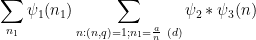
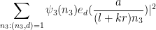
We want to understand how the convolution $\alpha * \psi_1 * \psi_2 * \psi_3$ is distributed in the residue class $a\ (d)$ , so we would like to compute the sum

$\sum_{n = a\ (d)} \alpha * \psi_1 * \psi_2 * \psi_3(n)$ .

with accuracy $o( MN_1N_2N_3 / d )$ . Fourier jnversion allows one to rewrite this expression as

$\frac{1}{d} \sum_h \sum_{n_2: (n_2,d)=1} \sum_{t: (t,d)=1} \hat \psi_1( \frac{h}{d}) \psi_2(n_2) \alpha*\psi_3(t) e_d( \frac{ah}{n_2t} )$

where

$\hat \psi_1(\theta) := \sum_{n_1} \psi_1(n_1) e(-n_1 \theta)$

is essentially of size $N_1$ when $\theta = O(1/N_1)$ and small elsewhere.

If we ignore all $h$ that are not coprime to $d$ , we may rearrange this as

$\sum_{l \in {\bf Z}/d{\bf Z}} \nu(l) F(l)$ (*)

where

$\nu(l) := \frac{1}{d} \sum_{h: (h,d)=1} \sum_{n_2: (n_2,d) = 1} 1_{\frac{n_2}{h} = l\ (d)} \hat \psi_1( \frac{ h }{d} ) \psi_2(n_2)$

and

$F(l) := 1_{(l,d)=1} \sum_{t: (t,d)=1} (\alpha * \psi_3)(t)e_d( \frac{a}{l t} )$ .

The function $\nu$ has a computable $\ell^2$ norm, basically

$\| \nu \|_{\ell^2}^2 \approx \frac{N_1 N_2}{d}$

and $F$ similarly has a computable $\ell^2$ norm by Plancherel:

$\|F\|_{\ell^2}^2 \approx M N_3 d.$ (**)

One could apply Cauchy-Schwarz directly to (*) to obtain an upper bound

$\|\nu\|_{\ell_2} \| F \|_{\ell^2}$ (***)

however this gives an unusable bound (unless we are in the Bombieri-Vinogradov range $d < \sqrt{x}$ ). To do better, Zhang notes that $\nu(l)$ has some smoothness, roughly speaking

$\nu(l) \approx \nu(l+k)$

whenever $k$ is an integer of size $O( N_1 N_2 / d )$ . This reflects the fact that the Farey sequence $\{ n_2/h: n_2 = O(N_2), h = O(d/N_1) \}$ is more or less stable with respect to shifts by integers $k$ of size $O(N_1 N_2/d)$ . This is basically all of the regularity that $\nu$ enjoys; one can compute the Fourier transform of $\nu$ in ${\bf Z}/d{\bf Z}$ to be spread out more or less evenly across frequencies of size $O( d^2 / N_1 N_2 )$ , save for a big concentration at the zero frequency mode of course.

The smoothness of $\nu$ allows one to approximately write (*) as

$\sum_{l \in ({\bf Z}/d{\bf Z})} \nu(l) {\bf E}_{k \in S} F(l+k)$

for any non-empty set $S$ of integers of size $O( N_1 N_2/d)$ , so we may replace (***) by the improved bound

$\|\nu\|_{\ell_2} \| {\bf E}_{k \in S} T_k F \|_{\ell^2}$ . (****)

where $T_k F(l) := F(l+k)$ is the translate of $F$ by $k$ . On the other hand, Bombieri-Birch/Ramanujan and completion of sums gives us a bound on the inner product

$\sum_{l \in {{\bf Z}/d{\bf Z}}} T_k F(l) T_{k'} F(l)$ ,

which is basically of the form

$M N_3 d ( \frac{(k-k',d)^{1/2}}{d^{1/2}} + \frac{M}{N_3} \frac{d^{1/2}}{(k-k',d)^{1/2}} )$ , (*****)

which is a bound which is strangely non-monotonic in $(k-k',d)$ : when $k-k'$ is divisible by d (and in particular in the diagonal case $k=k'$ ) it matches what one gets from Cauchy-Schwarz and (**) (this is basically why I got essentially no improvement by trying to treat the $k=k'$ case directly), then decreases as $k-k'$ becomes increasingly coprime with $d$ , until one reaches a transition and the bound worsens again as $(k-k',d)$ approaches 1. So to optimise in (****) one would like the differences $k-k'$ for $k,k' \in S$ to have some common factor with $d$ , but not too much of a factor, while also keeping $S$ reasonably large to avoid the diagonal terms from swamping everything; and so Zhang factors $d = qr$ for a controlled value of $r$ and sets $S$ to be the multiples of $r$ of size $O( N_1 N_2/d)$ . I think I’ve convinced myself that this is more or less the optimal choice of $S$ given the bounds available.

So it's the non-monotonicity of the bound (*****) that makes the argument slightly strange, but it appears difficult to improve upon (*****) without somehow gaining the ability to get bounds on short averages of Bombieri-Birch sums that improve upon the triangle inequality, which one can conjecture to be true (in the spirit of Hooley's conjecture) but it looks very difficult (and for this one should start with the Type I/II sums where one "only" has to deal with short averages of Kloosterman rather than short averages of Bombieri-Birch. I poked for a while on the Fourier side (replacing $l$ by its Fourier dual variable) to see if there was anything better than Weyl differencing available, but the only thing that seemed to suggest itself was bounds on higher moments (e.g. $\ell^4$ moment) of the Fourier transform of $F$ (or equivalently the $U^2$ Gowers norm of $F$ ), which didn't look very enticing. (In principle one gets more square root cancellation from increasingly higher-dimensional cases of the Weil conjectures, but this seems to be more than compensated for by the increased amount of completion of sums and Cauchy-Schwarz one has to perform.)

So, in summary, perhaps we've cleaned up all the low hanging fruit from Type III for now, and it's time to look again at Type I. I had a little look at the Ping Xi preprint giving some power savings on short Kloosterman sums, but have not yet worked out the numerology to see if the ranges in which Xi's bound are non-trivial are relevant here (and it's more "short averages of Kloosterman sums" that we need non-trivial bounds for rather than "short Kloosterman sums" per se).

18 June, 2013 at 6:19 pm

A truncated elementary Selberg sieve of Pintz | What's new

[…] that holds for as small as , but currently we are only able to establish this result for (see this comment). However, with the new truncated sieve of Pintz described in this post, we expect to be able to […]

20 June, 2013 at 9:45 am

Oktawian

Theorem 1 (Bounded gaps between primes) There exists a natural number {H} such that there are infinitely many pairs of distinct primes {p,q} with {|p-q| \leq H}.
I want to add some small observation about this theorem. If H is different than 3 that means there is not infinitly many pairs of even numbers like (n, n+2) and this unproven statement will be proven (or denied) if we will know the smallest H.

22 June, 2013 at 7:39 am

Bounding short exponential sums on smooth moduli via Weyl differencing | What's new

[…] in (using Lemma 5 from this previous post) we see that the total contribution to the off-diagonal case […]

22 June, 2013 at 8:01 am

Terence Tao

There is a new blog post of Emmanuel Kowalski at http://blogs.ethz.ch/kowalski/2013/06/22/bounded-gaps-between-primes-the-dawn-of-some-enlightenment/ announcing an improvement in the d_3 bounds on smooth moduli (which should also lead to improvements in the Type III bounds). Interestingly, Emmanuel claims that Weyl differencing may be avoided. He also mentions an older paper of Heath-Brown http://matwbn.icm.edu.pl/ksiazki/aa/aa47/aa4713.pdf that uses some similar ideas, I think I will try to look at that paper first.

23 June, 2013 at 9:14 pm

The distribution of primes in densely divisible moduli | What's new

[…] improves upon previous constraints of (see this blog comment) and (see Theorem 13 of this previous post), albeit for instead of . Inserting Theorem 4 into the […]

23 June, 2013 at 10:23 pm

Terence Tao

This thread and the companion Type I/II thread are being rolled over to

https://terrytao.wordpress.com/2013/06/23/the-distribution-of-primes-in-densely-divisible-moduli/

From past experience with polymath projects, now that our understanding of the project is more mature, the pace should settle down a bit from the crazily hectic pace of the last few weeks; I think we’re getting near the finish line and perhaps in a couple more weeks we will find a good place to “declare victory” and turn to the writing part of the project.

25 June, 2013 at 8:34 am

Zhang’s theorem on bounded prime gaps | random number theory generator

[…] Crucially, if is composite then we can surpass square root cancellation just slightly. […]

7 July, 2013 at 11:17 pm

The distribution of primes in doubly densely divisible moduli | What's new

[…] by Lemma 5 of this previous post and the bound is bounded […]

11 July, 2013 at 8:15 pm

Gergely Harcos

Minor correction: in the proof of Theorem 4, “ $C_p(a)$ equals […] $0$ when $a = 0\ (p)$ ” should be “ $C_p(a)$ equals […] $p-1$ when $a = 0\ (p)$ “.

[Corrected, thanks – T.]

	Yingyuan Li on Analysis II
	Anonymous on Analysis II
	Anonymous on Analysis II
	Yingyuan Li on Analysis II
	Yingyuan Li on Analysis II
	Yingyuan Li on Analysis II
	Yingyuan Li on Analysis II
	Jamie on On writing
	Anonymous on On writing
	Terence Tao on PCAST Working Group on Generat…
	Yingyuan Li on Analysis II
	Sam on 245A, Notes 5: Differentiation…
	Johan Aspegren on PCAST Working Group on Generat…
	Sam on 245A, Notes 5: Differentiation…
	wbshu on 247B, Notes 1: Restriction…

Estimation of the Type III sums

Recent Comments

Articles by others

Diversions

Mathematics

Selected articles

Software

The sciences

Top Posts

Archives

Categories

The Polymath Blog

83 comments

Leave a Reply Cancel reply

For commenters

Estimation of the Type III sums

Share this:

Like this:

Recent Comments

Articles by others

Diversions

Mathematics

Selected articles

Software

The sciences

Top Posts

Archives

Categories

The Polymath Blog

83 comments

Leave a Reply Cancel reply

For commenters