254A, Notes 3: The operator norm of a random matrix

9 January, 2010 in 254A - random matrices, math.PR, math.SP | Tags: Bai-Yin theorem, concentration of measure, epsilon net argument, iid matrices, moment method, operator norm, Wigner matrices | by Terence Tao

Now that we have developed the basic probabilistic tools that we will need, we now turn to the main subject of this course, namely the study of random matrices. There are many random matrix models (aka matrix ensembles) of interest – far too many to all be discussed in a single course. We will thus focus on just a few simple models. First of all, we shall restrict attention to square matrices ${M = (\xi_{ij})_{1 \leq i,j \leq n}}$ , where ${n}$ is a (large) integer and the ${\xi_{ij}}$ are real or complex random variables. (One can certainly study rectangular matrices as well, but for simplicity we will only look at the square case.) Then, we shall restrict to three main models:

Iid matrix ensembles, in which the coefficients ${\xi_{ij}}$ are iid random variables with a single distribution ${\xi_{ij} \equiv \xi}$ . We will often normalise ${\xi}$ to have mean zero and unit variance. Examples of iid models include the Bernouli ensemble (aka random sign matrices) in which the ${\xi_{ij}}$ are signed Bernoulli variables, the real gaussian matrix ensemble in which ${\xi_{ij} \equiv N(0,1)_{\bf R}}$ , and the complex gaussian matrix ensemble in which ${\xi_{ij} \equiv N(0,1)_{\bf C}}$ .
Symmetric Wigner matrix ensembles, in which the upper triangular coefficients ${\xi_{ij}}$ , ${j \geq i}$ are jointly independent and real, but the lower triangular coefficients ${\xi_{ij}}$ , ${j<i}$ are constrained to equal their transposes: ${\xi_{ij}=\xi_{ji}}$ . Thus ${M}$ by construction is always a real symmetric matrix. Typically, the strictly upper triangular coefficients will be iid, as will the diagonal coefficients, but the two classes of coefficients may have a different distribution. One example here is the symmetric Bernoulli ensemble, in which both the strictly upper triangular and the diagonal entries are signed Bernoulli variables; another important example is the Gaussian Orthogonal Ensemble (GOE), in which the upper triangular entries have distribution ${N(0,1)_{\bf R}}$ and the diagonal entries have distribution ${N(0,2)_{\bf R}}$ . (We will explain the reason for this discrepancy later.)
Hermitian Wigner matrix ensembles, in which the upper triangular coefficients are jointly independent, with the diagonal entries being real and the strictly upper triangular entries complex, and the lower triangular coefficients ${\xi_{ij}}$ , ${j<i}$ are constrained to equal their adjoints: ${\xi_{ij} = \overline{\xi_{ji}}}$ . Thus ${M}$ by construction is always a Hermitian matrix. This class of ensembles contains the symmetric Wigner ensembles as a subclass. Another very important example is the Gaussian Unitary Ensemble (GUE), in which all off-diagional entries have distribution ${N(0,1)_{\bf C}}$ , but the diagonal entries have distribution ${N(0,1)_{\bf R}}$ .

Given a matrix ensemble ${M}$ , there are many statistics of ${M}$ that one may wish to consider, e.g. the eigenvalues or singular values of ${M}$ , the trace and determinant, etc. In these notes we will focus on a basic statistic, namely the operator norm

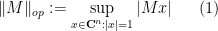
$\displaystyle \| M \|_{op} := \sup_{x \in {\bf C}^n: |x|=1} |Mx| \ \ \ \ \ (1)$

of the matrix ${M}$ . This is an interesting quantity in its own right, but also serves as a basic upper bound on many other quantities. (For instance, ${\|M\|_{op}}$ is also the largest singular value ${\sigma_1(M)}$ of ${M}$ and thus dominates the other singular values; similarly, all eigenvalues ${\lambda_i(M)}$ of ${M}$ clearly have magnitude at most ${\|M\|_{op}}$ .) Because of this, it is particularly important to get good upper tail bounds

$\displaystyle {\bf P}( \|M\|_{op} \geq \lambda ) \leq \ldots$

on this quantity, for various thresholds ${\lambda}$ . (Lower tail bounds are also of interest, of course; for instance, they give us confidence that the upper tail bounds are sharp.) Also, as we shall see, the problem of upper bounding ${\|M\|_{op}}$ can be viewed as a non-commutative analogue of upper bounding the quantity ${|S_n|}$ studied in Notes 1. (The analogue of the central limit theorem in Notes 2 is the Wigner semi-circular law, which will be studied in the next set of notes.)
An ${n \times n}$ matrix consisting entirely of ${1}$ s has an operator norm of exactly ${n}$ , as can for instance be seen from the Cauchy-Schwarz inequality. More generally, any matrix whose entries are all uniformly ${O(1)}$ will have an operator norm of ${O(n)}$ (which can again be seen from Cauchy-Schwarz, or alternatively from Schur’s test, or from a computation of the Frobenius norm). However, this argument does not take advantage of possible cancellations in ${M}$ . Indeed, from analogy with concentration of measure, when the entries of the matrix ${M}$ are independent, bounded and have mean zero, we expect the operator norm to be of size ${O(\sqrt{n})}$ rather than ${O(n)}$ . We shall see shortly that this intuition is indeed correct. (One can see, though, that the mean zero hypothesis is important; from the triangle inequality we see that if we add the all-ones matrix (for instance) to a random matrix with mean zero, to obtain a random matrix whose coefficients all have mean ${1}$ , then at least one of the two random matrices necessarily has operator norm at least ${n/2}$ .)
As mentioned before, there is an analogy here with the concentration of measure phenomenon, and many of the tools used in the latter (e.g. the moment method) will also appear here. (Indeed, we will be able to use some of the concentration inequalities from Notes 1 directly to help control ${\|M\|_{op}}$ and related quantities.) Similarly, just as many of the tools from concentration of measure could be adapted to help prove the central limit theorem, several the tools seen here will be of use in deriving the semi-circular law.
The most advanced knowledge we have on the operator norm is given by the Tracy-Widom law, which not only tells us where the operator norm is concentrated in (it turns out, for instance, that for a Wigner matrix (with some additional technical assumptions), it is concentrated in the range ${[2\sqrt{n} - O(n^{-1/6}), 2\sqrt{n} + O(n^{-1/6})]}$ ), but what its distribution in that range is. While the methods in this set of notes can eventually be pushed to establish this result, this is far from trivial, and will only be briefly discussed here. (We may return to the Tracy-Widom law later in this course, though.)

— 1. The epsilon net argument —

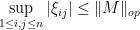
The slickest way to control ${\|M\|_{op}}$ is via the moment method. But let us defer using this method for the moment, and work with a more “naive” way to control the operator norm, namely by working with the definition (1). From that definition, we see that we can view the upper tail event ${\|M\|_{op} > \lambda}$ as a union of many simpler events:

$\displaystyle {\bf P}( \|M\|_{op} > \lambda ) \leq {\bf P}( \bigvee_{x \in S} |Mx| > \lambda ) \ \ \ \ \ (2)$

where ${S := \{x \in {\bf C}^d: |x|=1\}}$ is the unit sphere in the complex space ${{\bf C}^d}$ .
The point of doing this is that the event ${|Mx| > \lambda}$ is easier to control than the event ${\|M\|_{op} > \lambda}$ , and can in fact be handled by the concentration of measure estimates we already have. For instance:

Lemma 1 Suppose that the coefficients ${\xi_{ij}}$ of ${M}$ are independent, have mean zero, and uniformly bounded in magnitude by ${1}$ . Let ${x}$ be a unit vector in ${{\bf C}^n}$ . Then for sufficiently large ${A}$ (larger than some absolute constant), one has

$\displaystyle {\bf P}( |Mx| \geq A \sqrt{n} ) \leq C \exp( - c A^2 n )$

for some absolute constants ${C, c > 0}$ .

Proof: Let ${X_1,\ldots,X_n}$ be the ${n}$ rows of ${M}$ , then the column vector ${Mx}$ has coefficients ${X_i \cdot x}$ for ${i=1,\ldots,n}$ . if we let ${x_1,\ldots,x_n}$ be the coefficients of ${x}$ , so that ${\sum_{j=1}^n |x_j|^2 = 1}$ , then ${X_i \cdot x}$ is just ${\sum_{j=1}^n \xi_{ij} x_j}$ . Applying standard concentration of measure results (e.g. Exercise 4, Exercise 5, or Theorem 9 from Notes 1), we see that each ${X_i \cdot x}$ is uniformly subgaussian, thus

$\displaystyle {\bf P}( |X_i \cdot x| \geq \lambda ) \leq C \exp( - c \lambda^2 )$

for some absolute constants ${C, c > 0}$ . In particular, we have

$\displaystyle {\bf E} e^{c |X_i \cdot x|^2} \leq C$

for some (slightly different) absolute constants ${C, c > 0}$ . Multiplying these inequalities together for all ${i}$ , we obtain

$\displaystyle {\bf E} e^{c |Mx|^2} \leq C^n$

and the claim then follows from Markov’s inequality. $\Box$
Thus (with the hypotheses of Proposition 1), we see that for each individual unit vector ${x}$ , we have ${|Mx| = O(\sqrt{n})}$ with overwhelming probability. It is then tempting to apply the union bound and try to conclude that ${\|M\|_{op} = O(\sqrt{n})}$ with overwhelming probability also. However, we encounter a difficulty: the unit sphere ${S}$ is uncountable, and so we are taking the union over an uncountable number of events. Even though each event occurs with exponentially small probability, the union could well be everything.
Of course, it is extremely wasteful to apply the union bound to an uncountable union. One can pass to a countable union just by working with a countable dense subset of the unit sphere ${S}$ instead of the sphere itself, since the map ${x \mapsto |Mx|}$ is continuous. Of course, this is still an infinite set and so we still cannot usefully apply the union bound. However, the map ${x \mapsto |Mx|}$ is not just continuous; it is Lipschitz continuous, with a Lipschitz constant of ${\|M\|_{op}}$ . Now, of course there is some circularity here because ${\|M\|_{op}}$ is precisely the quantity we are trying to bound. Nevertheless, we can use this stronger continuity to refine the countable dense subset further, to a finite dense subset of ${S}$ , at the slight cost of modifying the threshold ${\lambda}$ by a constant factor. Namely:

Lemma 2 Let ${\Sigma}$ be a maximal ${1/2}$ -net of the sphere ${S}$ , i.e. a set of points in ${S}$ that are separated from each other by a distance of at least ${1/2}$ , and which is maximal with respect to set inclusion. Then for any ${n \times n}$ matrix ${M}$ with complex coefficients, and any ${\lambda > 0}$ , we have

$\displaystyle {\bf P}( \|M\|_{op} > \lambda ) \leq {\bf P}( \bigvee_{y \in \Sigma} |My| > \lambda/2 ).$

Proof: By (1) (and compactness) we can find ${x \in S}$ such that

$\displaystyle |Mx| = \|M\|_{op}.$

This point ${x}$ need not lie in ${\Sigma}$ . However, as ${\Sigma}$ is a maximal ${1/2}$ -net of ${S}$ , we know that ${x}$ lies within ${1/2}$ of some point ${y}$ in ${\Sigma}$ (since otherwise we could add ${x}$ to ${\Sigma}$ and contradict maximality). Since ${|x-y| \leq 1/2}$ , we have

$\displaystyle |M(x-y)| \leq \|M\|_{op}/2.$

By the triangle inequality we conclude that

$\displaystyle |My| \geq \|M\|_{op}/2.$

In particular, if ${\|M\|_{op} > \lambda}$ , then ${|My| > \lambda/2}$ for some ${y \in \Sigma}$ , and the claim follows. $\Box$

Remark 3 Clearly, if one replaces the maximal ${1/2}$ -net here with an maximal ${\varepsilon}$ -net for some other ${0<\varepsilon<1}$ (defined in the obvious manner), then we get the same conclusion, but with ${\lambda/2}$ replaced by ${\lambda (1-\varepsilon)}$ .

Now that we have discretised the range of points ${y}$ to be finite, the union bound becomes viable again. We first make the following basic observation:

Lemma 4 (Volume packing argument) Let ${0 < \varepsilon < 1}$ , and let ${\Sigma}$ be a ${\varepsilon}$ -net of the sphere ${S}$ . Then ${\Sigma}$ has cardinality at most ${(C/\varepsilon)^n}$ for some absolute constant ${C>0}$ .

Proof: Consider the balls of radius ${\varepsilon/2}$ centred around each point in ${\Sigma}$ ; by hypothesis, these are disjoint. On the other hand, by the triangle inequality, they are all contained in the ball of radius ${3/2}$ centred at the origin. The volume of the latter ball is at most ${(C/\varepsilon)^n}$ the volume of any of the small balls, and the claim follows. $\Box$

Exercise 5 Conversely, if ${\Sigma}$ is a maximal ${\varepsilon}$ -net, show that ${\Sigma}$ has cardinality at least ${(c/\varepsilon)^n}$ for some absolute constant ${c>0}$ .

And now we get an upper tail estimate:

Corollary 6 (Upper tail estimate for iid ensembles) Suppose that the coefficients ${\xi_{ij}}$ of ${M}$ are independent, have mean zero, and uniformly bounded in magnitude by ${1}$ . Then there exists absolute constants ${C, c > 0}$ such that

$\displaystyle {\bf P}( \|M\|_{op} > A \sqrt{n} ) \leq C \exp( - c A n )$

for all ${A \geq C}$ . In particular, we have ${\|M\|_{op} = O( \sqrt{n} )}$ with overwhelming probability.

Proof: From Lemma 2 and the union bound, we have

$\displaystyle {\bf P}( \|M\|_{op} > A \sqrt{n} ) \leq \sum_{y \in \Sigma} {\bf P}( |My| > A \sqrt{n}/2 )$

where ${\Sigma}$ is a maximal ${1/2}$ -net of ${S}$ . By Lemma 1, each of the probabilities ${{\bf P}( |My| > A \sqrt{n}/2 )}$ is bounded by ${C \exp( - c A n )}$ if ${A}$ is large enough. Meanwhile, from Lemma 4, ${\Sigma}$ has cardinality ${O(1)^n}$ . If ${A}$ is large enough, the entropy loss of ${O(1)^n}$ can be absorbed into the exponential gain of ${\exp(-c A n)}$ by modifying ${c}$ slightly, and the claim follows. $\Box$

Exercise 7 If ${\Sigma}$ is a maximal ${1/4}$ -net instead of a maximal ${1/2}$ -net, establish the following variant

$\displaystyle {\bf P}( \|M\|_{op} > \lambda ) \leq {\bf P}( \bigvee_{x,y \in \Sigma} |x^*My| > \lambda/4 )$

of Lemma 2. Use this to provide an alternate proof of Corollary 6.

The above result was for matrices with independent entries, but it easily extends to the Wigner case:

Corollary 8 (Upper tail estimate for Wigner ensembles) Suppose that the coefficients ${\xi_{ij}}$ of ${M}$ are independent for ${j \geq i}$ , mean zero, and uniformly bounded in magnitude by ${1}$ , and let ${\xi_{ij} := \overline{\xi_{ji}}}$ for ${j<i}$ . Then there exists absolute constants ${C, c > 0}$ such that

$\displaystyle {\bf P}( \|M\|_{op} > A \sqrt{n} ) \leq C \exp( - c A n )$

for all ${A \geq C}$ . In particular, we have ${\|M\|_{op} = O( \sqrt{n} )}$ with overwhelming probability.

Proof: From Corollary 6, the claim already holds for the upper-triangular portion of ${M}$ , as well as for the strict lower-triangular portion of ${M}$ . The claim then follows from the triangle inequality (adjusting the constants ${C, c}$ appropriately). $\Box$

Exercise 9 Generalise Corollary 6 and Corollary 8 to the case where the coefficients ${\xi_{ij}}$ have uniform subgaussian tails, rather than being uniformly bounded in magnitude by ${1}$ .

Remark 10 What we have just seen is a simple example of an epsilon net argument, which is useful when controlling a supremum of random variables ${\sup_{x \in S} X_x}$ such as (1), where each individual random variable ${X_x}$ is known to obey a large deviation inequality (in this case, Lemma 1). The idea is to use metric arguments (e.g. the triangle inequality, see Lemma 2) to refine the set of parameters ${S}$ to take the supremum over to an ${\varepsilon}$ -net ${\Sigma = \Sigma_\varepsilon}$ for some suitable ${\varepsilon}$ , and then apply the union bound. One takes a loss based on the cardinality of the ${\varepsilon}$ -net (which is basically the metric entropy or covering number of the original parameter space at scale ${\varepsilon}$ ), but one can hope that the bounds from the large deviation inequality are strong enough (and the metric entropy bounds sufficiently accurate) to overcome this entropy loss.
There is of course the question of what scale ${\varepsilon}$ to use. In this simple example, the scale ${\varepsilon=1/2}$ sufficed. In other contexts, one has to choose the scale ${\varepsilon}$ more carefully. In more complicated examples with no natural preferred scale, it often makes sense to take a large range of scales (e.g. ${\varepsilon = 2^{-j}}$ for ${j=1,\ldots,J}$ ) and chain them together by using telescoping series such as ${X_x = X_{x_1} + \sum_{j=1}^J X_{x_{j+1}} - X_{x_j}}$ (where ${x_j}$ is the nearest point in ${\Sigma_j}$ to ${x}$ for ${j=1,\ldots,J}$ , and ${x_{J+1}}$ is ${x}$ by convention) to estimate the supremum, the point being that one can hope to exploit cancellations between adjacent elements of the sequence ${X_{x_j}}$ . This is known as the method of chaining. There is an even more powerful refinement of this method, known as the method of generic chaining, which has a large number of applications; see this book by Talagrand for a beautiful and systematic treatment of the subject. However, we will not use this method in this course.

— 2. A symmetrisation argument (optional) —

We pause here to record an elegant symmetrisation argument that exploits convexity to allow us to reduce without loss of generality to the symmetric case ${M \equiv -M}$ , albeit at the cost of losing a factor of ${2}$ . We will not use this type of argument directly in these notes, but it is often used elsewhere in the literature.
Let ${M}$ be any random matrix with mean zero, and let ${\tilde M}$ be an independent copy of ${M}$ . Then, conditioning on ${M}$ , we have

$\displaystyle {\bf E} ( M - \tilde M | M ) = M.$

As the operator norm ${M \mapsto \|M\|_{op}}$ is convex, we can then apply Jensen’s inequality to conclude that

$\displaystyle {\bf E} ( \|M - \tilde M\|_{op} | M ) \geq \|M\|_{op}.$

Undoing the conditioning over ${M}$ , we conclude that

$\displaystyle {\bf E} \|M - \tilde M\|_{op} \geq {\bf E} \|M\|_{op}. \ \ \ \ \ (3)$

Thus, to upper bound the expected operator norm of ${M}$ , it suffices to upper bound the expected operator norm of ${M-\tilde M}$ . The point is that even if ${M}$ is not symmetric ( ${M \not \equiv -M}$ ), ${M - \tilde M}$ is automatically symmetric.
One can modify (3) in a few ways, given some more hypotheses on ${M}$ . Suppose now that ${M=(\xi_{ij})_{1 \leq i,j \leq n}}$ is a matrix with independent entries, thus ${M-\tilde M}$ has coefficients ${\xi_{ij}-\tilde \xi_{ij}}$ where ${\tilde \xi_{ij}}$ is an independent copy of ${\xi_{ij}}$ . Introduce a random sign matrix ${E = (\varepsilon_{ij})_{1 \leq i,j\leq n}}$ which is (jointly) independent of ${M, \tilde M}$ . Observe that as the distribution of ${\xi_{ij}-\tilde \xi_{ij}}$ is symmetric, that

$\displaystyle (\xi_{ij}-\tilde \xi_{ij}) \equiv (\xi_{ij}-\tilde \xi_{ij}) \varepsilon_{ij},$

and thus

$\displaystyle (M-\tilde M) \equiv (M - \tilde M) \cdot E$

where ${A \cdot B := (a_{ij} b_{ij})_{1\leq i,j \leq n}}$ is the Hadamard product of ${A = (a_{ij})_{1 \leq i,j \leq n}}$ and ${B = (b_{ij})_{1 \leq i,j \leq n}}$ . We conclude from (3) that

$\displaystyle {\bf E} \|M\|_{op} \leq {\bf E} \|(M - \tilde M) \cdot E\|_{op}.$

By the distributive law and the triangle inequality we have

$\displaystyle \|(M - \tilde M) \cdot E\|_{op} \leq \|M \cdot E\|_{op} + \|\tilde M \cdot E\|_{op}.$

But as ${M \cdot E \equiv \tilde M \cdot E}$ , the quantities ${\|M \cdot E\|_{op}}$ and ${\|\tilde M \cdot E\|_{op}}$ have the same expectation. We conclude the symmetrisation inequality

$\displaystyle {\bf E} \|M\|_{op} \leq 2 {\bf E} \| M \cdot E\|_{op}. \ \ \ \ \ (4)$

Thus, if one does not mind losing a factor of two, one has the freedom to randomise the sign of each entry of ${M}$ independently (assuming that the entries were already independent). Thus, in proving Corollary 6, one could have reduced to the case when the ${\xi_{ij}}$ were symmetric, though in this case this would not have made the argument that much simpler.
Sometimes it is preferable to multiply the coefficients by a Gaussian rather than by a random sign. Again, let ${M = (\xi_{ij})_{1 \leq i,j \leq n}}$ have independent entries with mean zero. Let ${G = (g_{ij})_{1 \leq i,j \leq n}}$ be a real gaussian matrix independent of ${M}$ , thus the ${g_{ij} \equiv N(0,1)_{\bf R}}$ are iid. We can split ${G = E \cdot |G|}$ , where ${E := ( \hbox{signum}(g_{ij}) )_{1 \leq i,j \leq n}}$ and ${|G| = (|g_{ij}|)_{1 \leq i,j \leq n}}$ . 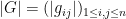Note that ${E}$ , ${M}$ , ${|G|}$ are independent, and ${E}$ is a random sign matrix. In particular, (4) holds. We now use

Exercise 11 If ${g \equiv N(0,1)_{\bf R}}$ , show that ${{\bf E} |g| = \sqrt{\frac{2}{\pi}}}$ .

From this exercise we see that

$\displaystyle {\bf E} (M \cdot E \cdot |G| | M, E ) = \sqrt{\frac{2}{\pi}} M \cdot E$

and hence by Jensen’s inequality again

$\displaystyle {\bf E} (\| M \cdot E \cdot |G|\|_{op} | M, E ) \geq \sqrt{\frac{2}{\pi}} \|M \cdot E\|_{op}.$

Undoing the conditional expectation in ${M, E}$ and applying (4) we conclude the gaussian symmetrisation inequality

$\displaystyle {\bf E} \|M\|_{op} \leq \sqrt{2\pi} {\bf E} \| M \cdot G\|_{op}. \ \ \ \ \ (5)$

Thus, for instance, when proving Corollary 6, one could have inserted a random gaussian in front of each coefficient. This would have made the proof of Lemma 1 marginally simpler (as one could compute directly with gaussians, and reduce the number of appeals to concentration of measure results) but in this case the improvement is negligible. In other situations though it can be quite helpful to have the additional random sign or random gaussian factor present. For instance, we have the following result of Latala:

Theorem 12 Let ${M = (\xi_{ij})_{1 \leq i,j \leq n}}$ be a matrix with independent mean zero entries, obeying the second moment bounds

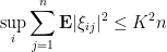
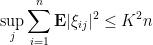
$\displaystyle \sup_i \sum_{j=1}^n {\bf E} |\xi_{ij}|^2 \leq K^2 n$

$\displaystyle \sup_j \sum_{i=1}^n {\bf E} |\xi_{ij}|^2 \leq K^2 n$

and the fourth moment bound

$\displaystyle \sum_{i=1}^n \sum_{j=1}^n {\bf E} |\xi_{ij}|^4 \leq K^4 n^2$

for some ${K>0}$ . Then ${{\bf E} \|M\|_{op} = O( K \sqrt{n} )}$ .

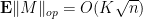Proof: (Sketch only) Using (5) one can replace ${\xi_{ij}}$ by ${\xi_{ij} \cdot g_{ij}}$ without much penalty. One then runs the epsilon-net argument with an explicit net, and uses concentration of measure results for gaussians (such as Theorem 8 from Notes 1) to obtain the analogue of Lemma 1. The details are rather intricate, and we refer the interested reader to Latala’s paper. $\Box$
As a corollary of Theorem 12, we see that if we have an iid matrix (or Wigner matrix) of mean zero whose entries have a fourth moment of ${O(1)}$ , then the expected operator norm is ${O(\sqrt{n})}$ . The fourth moment hypothesis is sharp. To see this, we make the trivial observation that the operator norm of a matrix ${M = (\xi_{ij})_{1 \leq i,j \leq n}}$ bounds the magnitude of any of its coefficients, thus

$\displaystyle \sup_{1 \leq i,j \leq n} |\xi_{ij}| \leq \|M\|_{op}$

or equivalently that

$\displaystyle {\bf P}(\|M\|_{op} \leq \lambda ) \leq {\bf P}(\bigvee_{1 \leq i,j \leq n} |\xi_{ij}| \leq \lambda).$

In the iid case ${\xi_{ij} \equiv \xi}$ , and setting ${\lambda = A \sqrt{n}}$ for some fixed ${A}$ independent of ${n}$ , we thus have

$\displaystyle {\bf P}(\|M\|_{op} \leq A \sqrt{n} ) \leq {\bf P}(|\xi| \leq A \sqrt{n})^{n^2} \ \ \ \ \ (6)$

With the fourth moment hypothesis, one has from dominated convergence that

$\displaystyle {\bf P}(|\xi| \leq A \sqrt{n}) \geq 1 - o_A(1/n^2),$

and so the right-hand side of (6) is asymptotically trivial. But with weaker hypotheses than the fourth moment hypothesis, the rate of convergence of ${{\bf P}(|\xi| \leq A \sqrt{n})}$ to ${1}$ can be slower, and one can easily build examples for which the right-hand side of (6) is ${o_A(1)}$ for every ${A}$ , which forces ${\|M\|_{op}}$ to typically be much larger than ${\sqrt{n}}$ on the average.

Remark 13 The symmetrisation inequalities remain valid with the operator norm replaced by any other convex norm on the space of matrices. The results are also just as valid for rectangular matrices as for square ones.

— 3. Concentration of measure —

Consider a random matrix ${M}$ of the type considered in Corollary 6 (e.g. a random sign matrix). We now know that the operator norm ${\|M\|_{op}}$ is of size ${O(\sqrt{n})}$ with overwhelming probability. But there is much more that can be said. For instance, by taking advantage of the convexity and Lipschitz properties of ${\|M\|_{op}}$ , we have the following quick application of Talagrand’s inequality (Theorem 9 from Notes 1):

Proposition 14 Let ${M}$ be as in Corollary 6. Then for any ${\lambda > 0}$ , one has

$\displaystyle {\bf P}( | \| M \|_{op} - {\bf M} \| M \|_{op} | \geq \lambda ) \leq C \exp(- c \lambda^2 )$

for some absolute constants ${C, c > 0}$ , where ${{\bf M} \|M\|_{op}}$ is a median value for ${\|M\|_{op}}$ . The same result also holds with ${{\bf M} \| M\|_{op}}$ replaced by the expectation ${{\bf E} \|M\|_{op}}$ .

Proof: We view ${\|M\|_{op}}$ as a function ${F( (\xi_{ij})_{1 \leq i,j \leq n} )}$ of the independent complex variables ${\xi_{ij}}$ , thus ${F}$ is a function from ${{\bf C}^{n^2}}$ to ${{\bf R}}$ . The convexity of the operator norm tells us that ${F}$ is convex. The triangle inequality, together with the elementary bound

$\displaystyle \|M\|_{op} \leq \|M\|_F \ \ \ \ \ (7)$

(easily proven by Cauchy-Schwarz), where

$\displaystyle \|M\|_F := (\sum_{i=1}^n \sum_{j=1}^n |\xi_{ij}|^2)^{1/2}$

is the Frobenius norm (also known as the Hilbert-Schmidt norm or ${2}$ -Schatten norm), tells us that ${F}$ is Lipschitz with constant ${1}$ . The claim then follows directly from Talagrand’s inequality. $\Box$

Exercise 15 Establish a similar result for the matrices in Corollary 8.

From Corollary 6 we know that the median or expectation of ${\|M\|_{op}}$ is of size ${O(\sqrt{n})}$ ; we now know that ${\|M\|_{op}}$ concentrates around this median to width at most ${O(1)}$ . (This turns out to be non-optimal; the Tracy-Widom law actually gives a concentration of ${O(n^{-1/6})}$ , under some additional assumptions on ${M}$ . Nevertheless this level of concentration is already non-trivial.)
However, this argument does not tell us much about what the median or expected value of ${\|M\|_{op}}$ actually is. For this, we will need to use other methods, such as the moment method which we turn to next.

Remark 16 Talagrand’s inequality, as formulated in these notes, relies heavily on convexity. Because of this, we cannot apply this argument directly to non-convex matrix statistics, such as singular values ${\sigma_j(M)}$ other than the largest singular value ${\sigma_1(M)}$ . Nevertheless, one can still use this inequality to obtain good concentration results, by using the convexity of related quantities, such as the partial sums ${\sum_{j=1}^J \sigma_j(M)}$ ; see this paper of Meckes. Other approaches include the use of alternate large deviation inequalities, such as those arising from log-Sobolev inequalities (see e.g. this book by Guionnet), or by using more abstract versions of Talagrand’s inequality (see this paper of Alon, Krivelevich, and Vu).

— 4. The moment method —

We now bring the moment method to bear on the problem, starting with the easy moments and working one’s way up to the more sophisticated moments. It turns out that it is easier to work first with the case when ${M}$ is symmetric or Hermitian; we will discuss the non-symmetric case near the end of these notes.
The starting point for the moment method is the observation that for symmetric or Hermitian ${M}$ , the operator norm ${\|M\|_{op}}$ is equal to the ${\ell^\infty}$ norm

$\displaystyle \|M\|_{op} = \max_{1 \leq i \leq n} |\lambda_i| \ \ \ \ \ (8)$

of the eigenvalues ${\lambda_1,\ldots,\lambda_n\in {\bf R}}$ of ${M}$ . On the other hand, we have the standard linear algebra identity

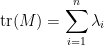
$\displaystyle \hbox{tr}(M) = \sum_{i=1}^n \lambda_i$

and more generally

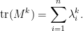
$\displaystyle \hbox{tr}(M^k) = \sum_{i=1}^n \lambda_i^k.$

In particular, if ${k=2,4,\ldots}$ is an even integer, then ${\hbox{tr}(M^k)^{1/k}}$ is just the ${\ell^k}$ norm of these eigenvalues, and we have the inequalities

$\displaystyle \| M \|_{op}^k \leq \hbox{tr}(M^k) \leq n \|M\|_{op}^k. \ \ \ \ \ (9)$

To put this another way, knowledge of the ${k^{th}}$ moment ${\hbox{tr}(M^k)}$ controls the operator norm up to a multiplicative factor of ${n^{1/k}}$ . Taking larger and larger ${k}$ , we should thus obtain more accurate control on the operator norm. (This is basically the philosophy underlying the power method.)

Remark 17 In most cases, one expects the eigenvalues to be reasonably uniformly distributed, in which case the upper bound in (9) is closer to the truth than the lower bound. One scenario in which this can be rigorously established is if it is known that the eigenvalues of ${M}$ all come with a high multiplicity. This is often the case for matrices associated with group actions (particularly those which are quasirandom in the sense of Gowers). However, this is usually not the case with most random matrix ensembles, and we must instead proceed by increasing ${k}$ as described above.

Let’s see how this method works in practice. The simplest case is that of the second moment ${\hbox{tr}(M^2)}$ , which in the Hermitian case works out to

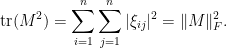
$\displaystyle \hbox{tr}(M^2) = \sum_{i=1}^n \sum_{j=1}^n |\xi_{ij}|^2 = \|M\|_F^2.$

(Thus we see that (7) is just the ${k=2}$ case of the lower inequality in (9), at least in the Hermitian case.)
The expression ${\sum_{i=1}^n \sum_{j=1}^n |\xi_{ij}|^2}$ is easy to compute in practice. For instance, for the symmetric Bernoulli ensemble, this expression is exactly equal to ${n^2}$ . More generally, if we have a Wigner matrix in which all off-diagonal entries have mean zero and unit variance, and the diagonal entries have mean zero and bounded variance (this is the case for instance for GOE), then the off-diagonal entries have mean ${1}$ , and by the law of large numbers we see that this expression is almost surely asymptotic to ${n^2}$ . (There is of course a dependence between the upper triangular and lower triangular entries, but this is easy to deal with by folding the sum into twice the upper triangular portion (plus the diagonal portion, which is lower order).)
From the weak law of large numbers, we see in particular that one has

$\displaystyle \sum_{i=1}^n \sum_{j=1}^n |\xi_{ij}|^2 = (1+o(1)) n^2 \ \ \ \ \ (10)$

asymptotically almost surely.

Exercise 18 If the ${\xi_{ij}}$ have uniformly sub-exponential tail, show that we in fact have (10) with overwhelming probability.

Applying (9), we obtain the bounds

$\displaystyle (1+o(1)) \sqrt{n} \leq \|M\|_{op} \leq (1+o(1)) n \ \ \ \ \ (11)$

asymptotically almost surely. This is already enough to show that the median of ${\|M\|_{op}}$ is at least ${(1+o(1)) \sqrt{n}}$ , which complements (up to constants) the upper bound of ${O(\sqrt{n})}$ obtained from the epsilon net argument. But the upper bound here is terrible; we will need to move to higher moments to improve it.
Accordingly, we now turn to the fourth moment. For simplicity let us assume that all entries ${\xi_{ij}}$ have zero mean and unit variance. To control moments beyond the second moment, we will also assume that all entries are bounded in magnitude by some ${K}$ . We expand

$\displaystyle \hbox{tr}(M^4) = \sum_{1 \leq i_1,i_2,i_3,i_4 \leq n} \xi_{i_1 i_2} \xi_{i_2 i_3} \xi_{i_3 i_4} \xi_{i_4 i_1}.$

To understand this expression, we take expectations:

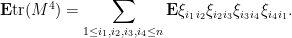
$\displaystyle {\bf E} \hbox{tr}(M^4) = \sum_{1 \leq i_1,i_2,i_3,i_4 \leq n} {\bf E} \xi_{i_1 i_2} \xi_{i_2 i_3} \xi_{i_3 i_4} \xi_{i_4 i_1}.$

One can view this sum graphically, as a sum over length four cycles in the vertex set ${\{1,\ldots,n\}}$ ; note that the four edges ${\{i_1,i_2\}, \{i_2,i_3\}, \{i_3,i_4\}, \{i_4,i_1\}}$ are allowed to be degenerate if two adjacent ${\xi_i}$ are equal. The value of each term

$\displaystyle {\bf E} \xi_{i_1 i_2} \xi_{i_2 i_3} \xi_{i_3 i_4} \xi_{i_4 i_1} \ \ \ \ \ (12)$

in this sum depends on what the cycle does.
Firstly, there is the case when all the four edges ${\{i_1,i_2\}, \{i_2,i_3\}, \{i_3,i_4\}, \{i_4,i_1\}}$ are distinct. Then the four factors ${\xi_{i_1 i_2},\ldots,\xi_{i_4 i_1}}$ are independent; since we are assuming them to have mean zero, the term (12) vanishes. Indeed, the same argument shows that the only terms that do not vanish are those in which each edge is repeated at least twice. A short combinatorial case check then shows that, up to cyclic permutations of the ${i_1,i_2,i_3,i_4}$ indices there are now only a few types of cycles in which the term (12) does not automatically vanish:

${i_1=i_3}$ , but ${i_2, i_4}$ are distinct from each other and from ${i_1}$ .
${i_1=i_3}$ and ${i_2=i_4}$ .
${i_1=i_2=i_3}$ , but ${i_4}$ is distinct from ${i_1}$ .
${i_1=i_2=i_3=i_4}$ .

In the first case, the independence and unit variance assumptions tells us that (12) is ${1}$ , and there are ${O(n^3)}$ such terms, so the total contribution here to ${{\bf E} \hbox{tr}(M^4)}$ is at most ${O(n^3)}$ . In the second case, the unit variance and bounded by ${K}$ tells us that the term is ${O(K^2)}$ , and there are ${O(n^2)}$ such terms, so the contribution here is ${O(n^2 K^2)}$ . Similarly, the contribution of the third type of cycle is ${O(n^2)}$ , and the fourth type of cycle is ${O(n K^2)}$ , so we can put it all together to get

$\displaystyle {\bf E} \hbox{tr}(M^4) \leq O( n^3 ) + O( n^2 K^2 ).$

In particular, if we make the hypothesis ${K = O(\sqrt{n})}$ , then we have

$\displaystyle {\bf E} \hbox{tr}(M^4) \leq O(n^3),$

and thus by Markov’s inequality we see that for any ${\varepsilon > 0}$ , ${\hbox{tr}(M^4) \leq O_\varepsilon(n^3)}$ with probability at least ${1-\varepsilon}$ . Applying (9), this leads to the upper bound

$\displaystyle \| M \|_{op} \leq O_\varepsilon( n^{3/4} )$

with probability at least ${1-\varepsilon}$ ; a similar argument shows that for any fixed ${\varepsilon > 0}$ , one has

$\displaystyle \| M \|_{op} \leq n^{3/4+\varepsilon}$

with high probability. This is better than the upper bound obtained from the second moment method, but still non-optimal.

Exercise 19 If ${K = o(\sqrt{n})}$ , use the above argument to show that

$\displaystyle ({\bf E} \|M\|_{op}^4)^{1/4} \geq (2^{1/4}+o(1)) \sqrt{n}$

which in some sense improves upon (11) by a factor of ${2^{1/4}}$ . In particular, if ${K = O(1)}$ , conclude that the median of ${\|M\|_{op}}$ is at least ${(2^{1/4}+o(1)) \sqrt{n}}$ .

Now let us take a quick look at the sixth moment, again with the running assumption of a Wigner matrix in which all entries have mean zero, unit variance, and bounded in magnitude by ${K}$ . We have

$\displaystyle {\bf E} \hbox{tr}(M^6) = \sum_{1 \leq i_1,\ldots,i_6 \leq n} {\bf E} \xi_{i_1 i_2} \ldots \xi_{i_5 i_6} \xi_{i_6 i_1},$

a sum over cycles of length ${6}$ in ${\{1,\ldots,n\}}$ . Again, most of the summands here vanish; the only ones which do not are those cycles in which each edge occurs at least twice (so in particular, there are at most three distinct edges).
Classifying all the types of cycles that could occur here is somewhat tedious, but it is clear that there are going to be ${O(1)}$ different types of cycles. But we can organise things by the multiplicity of each edge, leaving us with four classes of cycles to deal with:

Cycles in which there are three distinct edges, each occuring two times.
Cycles in which there are two distinct edges, one occuring twice and one occuring four times.
Cycles in which there are two distinct edges, each occuring three times. (Actually, this case ends up being impossible, due to a “bridges of Königsberg” type of obstruction, but we will retain it for this discussion.)
Cycles in which a single edge occurs six times.

It is not hard to see that summands coming from the first type of cycle give a contribution of ${1}$ , and there are ${O(n^4)}$ of these (because such cycles span at most four vertices). Similarly, the second and third types of cycles give a contribution of ${O( K^2 )}$ per summand, and there are ${O( n^3 )}$ summands; finally, the fourth type of cycle gives a contribution of ${O( K^4 )}$ , with ${O(n^2)}$ summands. Putting this together we see that

$\displaystyle {\bf E} \hbox{tr}(M^6) \leq O( n^4 ) + O( n^3 K^2 ) + O( n^2 K^4 );$

so in particular if we assume ${K = O(\sqrt{n})}$ as before, we have

$\displaystyle {\bf E} \hbox{tr}(M^6) \leq O( n^4 )$

and if we then use (9) as before we see that

$\displaystyle \| M \|_{op} \leq O_\varepsilon( n^{2/3} )$

with probability ${1-\varepsilon}$ , for any ${\varepsilon > 0}$ ; so we are continuing to make progress towards what we suspect (from the epsilon net argument) to be the correct bound of ${n^{1/2}}$ .

Exercise 20 If ${K = o(\sqrt{n})}$ , use the above argument to show that

$\displaystyle ({\bf E} \|M\|_{op}^6)^{1/6} \geq (5^{1/6}+o(1)) \sqrt{n}.$

In particular, if ${K = O(1)}$ , conclude that the median of ${\|M\|_{op}}$ is at least ${(5^{1/6}+o(1)) \sqrt{n}}$ . Thus this is a (slight) improvement over Exercise 19.

Let us now consider the general ${k^{th}}$ moment computation under the same hypotheses as before, with ${k}$ an even integer, and make some modest attempt to track the dependency of the constants on ${k}$ . Again, we have

$\displaystyle {\bf E} \hbox{tr}(M^k) = \sum_{1 \leq i_1,\ldots,i_k \leq n} {\bf E} \xi_{i_1 i_2} \ldots \xi_{i_k i_1}, \ \ \ \ \ (13)$

which is a sum over cycles of length ${k}$ . Again, the only non-vanishing expectations are those for which each edge occurs twice; in particular, there are at most ${k/2}$ edges, and thus at most ${k/2+1}$ vertices.
We divide the cycles into various classes, depending on which edges are equal to each other. (More formally, a class is an equivalence relation ${\sim}$ on a set of ${k}$ labels, say ${\{1,\ldots,k\}}$ in which each equivalence class contains at least two elements, and a cycle of ${k}$ edges ${\{i_1,i_2\},\ldots,\{i_k,i_1\}}$ lies in the class associated to ${\sim}$ when we have that ${\{ i_j,i_{j+1} \} = \{i_{j'},i_{j'+1}\}}$ iff ${j \sim j'}$ , where we adopt the cyclic notation ${i_{k+1} := i_1}$ .)
How many different classes could there be? We have to assign up to ${k/2}$ labels to ${k}$ edges, so a crude upper bound here is ${(k/2)^{k}}$ .
Now consider a given class of cycle. It has ${j}$ edges ${e_1,\ldots,e_j}$ for some ${1 \leq j \leq k/2}$ , with multiplicities ${a_1,\ldots,a_j}$ , where ${a_1,\ldots,a_j}$ are at least ${2}$ and add up to ${k}$ . The ${j}$ edges span at most ${j+1}$ vertices; indeed, in addition to the first vertex ${i_1}$ , one can specify all the other vertices by looking at the first appearance of each of the ${j}$ edges ${e_1,\ldots,e_j}$ in the path from ${i_1}$ to ${i_k}$ , and recording the final vertex of each such edge. From this, we see that the total number of cycles in this particular class is at most ${n^{j+1}}$ . On the other hand, because each ${\xi_{ij}}$ has mean zero, unit variance and is bounded by ${K}$ , the ${a^{th}}$ moment of this coefficient is at most ${K^{a-2}}$ for any ${a \geq 2}$ . Thus each summand in (13) coming from a cycle in this class has magnitude at most

$\displaystyle K^{a_1-2} \ldots K^{a_j-2} = K^{a_1+\ldots+a_j-2j} = K^{k-2j}.$

Thus the total contribution of this class to (13) is ${n^{j+1} K^{k-2j}}$ , which we can upper bound by

$\displaystyle \max(n^{\frac{k}{2}+1}, n^2 K^{k-2} ) = n^{k/2 + 1} \max( 1, K/\sqrt{n} )^{k-2}.$

Summign up over all classes, we obtain the (somewhat crude) bound

$\displaystyle {\bf E} \hbox{tr}(M^k) \leq (k/2)^k n^{k/2+1} \max( 1, K/\sqrt{n} )^{k-2}$

and thus by (9)

$\displaystyle {\bf E} \|M\|_{op}^k \leq (k/2)^k n^{k/2+1} \max( 1, K/\sqrt{n} )^{k-2}$

and so by Markov’s inequality we have

$\displaystyle {\bf P}( \|M\|_{op} \geq \lambda ) \leq \lambda^{-k} (k/2)^k n^{k/2+1} \max( 1, K/\sqrt{n} )^{k-2}$

for all ${\lambda > 0}$ . This, for instance, places the median of ${\|M\|_{op}}$ at ${O( n^{1/k} k \sqrt{n} \max(1, K/\sqrt{n}) )}$ . We can optimise this in ${k}$ by choosing ${k}$ to be comparable to ${\log n}$ , and so we obtain an upper bound of ${O( \sqrt{n} \log n \max(1, K/\sqrt{n}) )}$ for the median; indeed, a slight tweaking of the constants tells us that ${\|M\|_{op} = O( \sqrt{n} \log n \max(1, K/\sqrt{n}) )}$ with high probability.
The same argument works if the entries have at most unit variance rather than unit variance, thus we have shown

Proposition 21 (Weak upper bound) Let ${M}$ be a random Hermitian matrix, with the upper triangular entries ${\xi_{ij}}$ , ${i \leq j}$ being independent with mean zero and variance at most ${1}$ , and bounded in magnitude by ${K}$ . Then ${\|M\|_{op} = O( \sqrt{n} \log n \max(1, K/\sqrt{n}) )}$ with high probability.

When ${K \leq \sqrt{n}}$ , this gives an upper bound of ${O(\sqrt{n} \log n)}$ , which is still off by half a logarithm from the expected bound of ${O(\sqrt{n})}$ . We will remove this half-logarithmic loss later in these notes.

— 5. Computing the moment to top order —

Now let us consider the case when ${K = o(\sqrt{n})}$ , and each entry has variance exactly ${1}$ . We have an upper bound

$\displaystyle {\bf E} \hbox{tr}(M^k) \leq (k/2)^k n^{k/2+1};$

let us try to get a more precise answer here (as in Exercises 19, 20). Recall that each class of cycle contributed a bound of ${n^{j+1} K^{k-2j}}$ to this expression. If ${K = o(\sqrt{n})}$ , we see that such expressions are ${o_k(n^{k/2+1})}$ whenever ${j < k/2}$ , where the ${o_k()}$ notation means that the decay rate as ${n \rightarrow \infty}$ can depend on ${k}$ . So the total contribution of all such classes is ${o_k(n^{k/2+1})}$ .
Now we consider the remaining classes with ${j=k/2}$ . For such classes, each equivalence class of edges contains exactly two representatives, thus each edge is repeated exactly once. The contribution of each such cycle to (13) is exactly ${1}$ , thanks to the unit variance and independence hypothesis. Thus, the total contribution of these classes to ${{\bf E} \hbox{tr}(M^k)}$ is equal to a purely combinatorial quantity, namely the number of cycles of length ${k}$ on ${\{1,\ldots,n\}}$ in which each edge is repeated exactly once, yielding ${k/2}$ unique edges. We are thus faced with the enumerative combinatorics problem of bounding this quantity as precisely as possible.
With ${k/2}$ edges, there are at most ${k/2+1}$ vertices traversed by the cycle. If there are fewer than ${k/2+1}$ vertices traversed, then there are at most ${O_k(n^{k/2}) = o_k(n^{k/2+1})}$ cycles of this type, since one can specify such cycles by identifying up to ${k/2}$ vertices in ${\{1,\ldots,n\}}$ and then matching those coordinates with the ${k}$ vertices of the cycle. So we set aside these cycles, and only consider those cycles which traverse exactly ${k/2+1}$ vertices. Let us call such cycles (i.e. cycles of length ${k}$ with each edge repeated exactly once, and traversing exactly ${k/2+1}$ vertices) non-crossing cycles of length ${k}$ in ${\{1,\ldots,n\}}$ . Our remaining task is then to count the number of non-crossing cycles.

Example 22 Let ${a,b,c,d}$ be distinct elements of ${\{1,\ldots,n\}}$ . Then ${(i_1,\ldots,i_6) = (a,b,c,d,c,b)}$ is a non-crossing cycle of length ${k}$ , as is ${(a,b,a,c,a,d)}$ . Any cyclic permutation of a non-crossing cycle is again a non-crossing cycle.

Exercise 23 Show that a cycle of length ${k}$ is non-crossing if and only if there exists a tree in ${\{1,\ldots,n\}}$ of ${k/2}$ edges and ${k/2+1}$ vertices, such that the cycle lies in the tree and traverses each edge in the tree exactly twice.

Exercise 24 Let ${i_1,\ldots,i_k}$ be a cycle of length ${k}$ . Arrange the integers ${1,\ldots,k}$ around a circle, and draw a line segment between two distinct integers ${1 \leq a < b \leq k}$ whenever ${i_a=i_b}$ , with no ${c}$ between ${a,b}$ for which ${i_a=i_c=i_b}$ . Show that the cycle is non-crossing if and only if the number of line segments is exactly ${k/2-1}$ , and the line segments do not cross each other. This may help explain the terminology “non-crossing”.

Now we can complete the count. If ${k}$ is a positive even integer, define a Dyck word of length ${k}$ to be the number of words consisting of left and right parentheses (, ) of length ${k}$ , such that when one reads from left to right, there are always at least as many left parentheses as right parentheses (or in other words, the parentheses define a valid nesting). For instance, the only Dyck word of length ${2}$ is ${()}$ , the two Dyck words of length ${4}$ are ${(())}$ and ${()()}$ , and the five Dyck words of length ${6}$ are

$\displaystyle ()()(), (())(), ()(()), (()()), ((())),$

and so forth. (Dyck words are also closely related to Dyck paths.)

Lemma 25 The number of non-crossing cycles of length ${k}$ in ${\{1,\ldots,n\}}$ is equal to ${C_{k/2} n (n-1) \ldots (n-k/2)}$ , where ${C_{k/2}}$ is the number of Dyck words of length ${k}$ . (The number ${C_{k/2}}$ is also known as the ${(k/2)^{th}}$ Catalan number.)

Proof: We will give a bijective proof. Namely, we will find a way to store a non-crossing cycle as a Dyck word, together with an (ordered) sequence of ${k/2+1}$ distinct elements from ${\{1,\ldots,n\}}$ , in such a way that any such pair of a Dyck word and ordered sequence generates exactly one non-crossing cycle. This will clearly give the claim.
So, let us take a non-crossing cycle ${i_1,\ldots,i_k}$ . We imagine traversing this cycle from ${i_1}$ to ${i_2}$ , then from ${i_2}$ to ${i_3}$ , and so forth until we finally return to ${i_1}$ from ${i_k}$ . On each leg of this journey, say from ${i_j}$ to ${i_{j+1}}$ , we either use an edge that we have not seen before, or else we are using an edge for the second time. Let us say that the leg from ${i_j}$ to ${i_{j+1}}$ is an innovative leg if it is in the first category, and a returning leg otherwise. Thus there are ${k/2}$ innovative legs and ${k/2}$ returning legs. Clearly, it is only the innovative legs that can bring us to vertices that we have not seen before. Since we have to visit ${k/2+1}$ distinct vertices (including the vertex ${i_1}$ we start at), we conclude that each innovative leg must take us to a new vertex. We thus record, in order, each of the new vertices we visit, starting at ${i_1}$ and adding another vertex for each innovative leg; this is an ordered sequence of ${k/2+1}$ distinct elements of ${\{1,\ldots,n\}}$ . Next, traversing the cycle again, we write down a ${(}$ whenever we traverse an innovative leg, and an ${)}$ otherwise. This is clearly a Dyck word. For instance, using the examples in Example 22, the non-crossing cycle ${(a,b,c,d,c,b)}$ gives us the ordered sequence ${(a,b,c,d)}$ and the Dyck word ${((()))}$ , while ${(a,b,a,c,a,d)}$ gives us the ordered sequence ${(a,b,c,d)}$ and the Dyck word ${()()()}$ .
We have seen that every non-crossing cycle gives rise to an ordered sequence and a Dyck word. A little thought shows that the cycle can be uniquely reconstructed from this ordered sequence and Dyck word (the key point being that whenever one is performing a returning leg from a vertex ${v}$ , one is forced to return along the unique innovative leg that discovered ${v}$ ). A slight variant of this thought also shows that every Dyck word of length ${k}$ and ordered sequence of ${k/2+1}$ distinct elements gives rise to a non-crossing cycle. This gives the required bijection, and the claim follows. $\Box$
Next, we recall the classical formula for the Catalan number:

Exercise 26 Establish the recurrence

$\displaystyle C_{n+1} = \sum_{i=0}^{n} C_i C_{n-i}$

for any ${n \geq 1}$ (with the convention ${C_0=1}$ ), and use this to deduce that

$\displaystyle C_{k/2} := \frac{k!}{(k/2+1)! (k/2)!} \ \ \ \ \ (14)$

for all ${k=2,4,6,\ldots}$ .

Exercise 27 Let ${k}$ be a positive even integer. Given a string of ${k/2}$ left parentheses and ${k/2}$ right parentheses which is not a Dyck word, define the reflection of this string by taking the first right parenthesis which does not have a matching left parenthesis, and then reversing all the parentheses after that right parenthesis. Thus, for instance, the reflection of ${())(()}$ is ${())))(}$ . Show that there is a bijection between non-Dyck words with ${k/2}$ left parentheses and ${k/2}$ right parentheses, and arbitrary words with ${k/2-1}$ left parentheses and ${k/2+1}$ right parentheses. Use this to give an alternate proof of (14).

Note that ${n(n-1)\ldots(n-k/2) = (1+o_k(1)) n^{k/2+1}}$ . Putting all the above computations together, we conclude

Theorem 28 (Moment computation) Let ${M}$ be a real symmetric random matrix, with the upper triangular elements ${\xi_{ij}}$ , ${i \leq j}$ jointly independent with mean zero and variance one, and bounded in magnitude by ${o( \sqrt{n})}$ . Let ${k}$ be a positive even integer. Then we have

$\displaystyle {\bf E} \hbox{tr}(M^k) = (C_{k/2} + o_k(1)) n^{k/2+1}$

where ${C_{k/2}}$ is given by (14).

Remark 29 An inspection of the proof also shows that if we allow the ${\xi_{ij}}$ to have variance at most one, rather than equal to one, we obtain the upper bound

$\displaystyle {\bf E} \hbox{tr}(M^k) \leq (C_{k/2} + o_k(1)) n^{k/2+1}.$

Exercise 30 Show that Theorem 28 also holds for Hermitian random matrices. (Hint: The main point is that with non-crossing cycles, each non-innovative leg goes in the reverse direction to the corresponding innovative leg – why?)

Remark 31 Theorem 28 can be compared with the formula

$\displaystyle {\bf E} S^k = (C'_{k/2} + o_k(1)) n^{k/2}$

derived in Notes 1, where ${S = X_1 + \ldots + X_n}$ is the sum of ${n}$ iid random variables of mean zero and variance one, and

$\displaystyle C'_{k/2} := \frac{k!}{2^{k/2} (k/2)!}.$

Exercise 24 shows that ${C_{k/2}}$ can be interpreted as the number of ways to join ${k}$ points on the circle by ${k/2-1}$ non-crossing chords. In a similar vein, ${C'_{k/2}}$ can be interpreted as the number of ways to join ${k}$ points on the circle by ${k/2}$ chords which are allowed to cross each other (except at the endpoints). Thus moments of Wigner-type matrices are in some sense the “non-crossing” version of moments of sums of random variables. We will discuss this phenomenon more when we turn to free probability in later notes.

Combining Theorem 28 with (9) we obtain a lower bound

$\displaystyle {\bf E} \|M\|_{op}^k \geq (C_{k/2}+o_k(1)) n^{k/2}.$

In the bounded case ${K=O(1)}$ , we can combine this with Exercise 15 to conclude that the median (or mean) of ${\|M\|_{op}}$ is at least ${(C_{k/2}^{1/k}+o_k(1)) \sqrt{n}}$ . On the other hand, from Stirling’s formula (Notes 0a) we see that ${C_{k/2}^{1/k}}$ converges to ${2}$ as ${k \rightarrow \infty}$ . Taking ${k}$ to be a slowly growing function of ${n}$ , we conclude

Proposition 32 (Lower bound) Let ${M}$ be a real symmetric random matrix, with the upper triangular elements ${\xi_{ij}}$ , ${i \leq j}$ jointly independent with mean zero and variance one, and bounded in magnitude by ${O(1)}$ . Then the median (or mean) of ${\|M\|_{op}}$ is at least ${(2-o(1)) \sqrt{n}}$ .

Remark 33 One can in fact obtain an exact asymptotic expansion of the moments ${{\bf E} \hbox{tr}(M^k)}$ as a polynomial in ${n}$ , known as the genus expansion of the moments. This expansion is however somewhat difficult to work with from a combinatorial perspective (except at top order) and will not be used here.

— 6. Removing the logarithm —

The upper bound in Proposition 21 loses a logarithm in comparison to the lower bound coming from Theorem 28. We now discuss how to remove this logarithm.
Suppose that we could eliminate the ${o_k(1)}$ error in Theorem 28. Then from (9) we would have

$\displaystyle {\bf E} \|M\|_{op}^k \leq C_{k/2} n^{k/2+1}$

and hence by Markov’s inequality

$\displaystyle {\bf P}(\|M\|_{op} > \lambda) \leq \lambda^{-k} C_{k/2} n^{k/2+1}.$

Applying this with ${\lambda = (2+\varepsilon) \sqrt{n}}$ for some fixed ${\varepsilon > 0}$ , and setting ${k}$ to be a large multiple of ${\log n}$ , we see that ${\|M\|_{op} \leq (2 + O(\varepsilon)) \sqrt{n}}$ asymptotically almost surely, which on selecting ${\varepsilon}$ to grow slowly in ${n}$ gives in fact that ${\|M\|_{op} \leq (2+o(1)) \sqrt{n}}$ asymptotically almost surely, thus complementing the lower bound in Proposition 32.
This argument was not rigorous because it did not address the ${o_k(1)}$ error. Without a more quantitative accounting of this error, one cannot set ${k}$ as large as ${\log n}$ without losing control of the error terms; and indeed, a crude accounting of this nature will lose factors of ${k^k}$ which are unacceptable. Nevertheless, by tightening the hypotheses a little bit and arguing more carefully, we can get a good bound, for ${k}$ in the region of interest:

Theorem 34 (Improved moment bound) Let ${M}$ be a real symmetric random matrix, with the upper triangular elements ${\xi_{ij}}$ , ${i \leq j}$ jointly independent with mean zero and variance one, and bounded in magnitude by ${O(n^{0.49})}$ (say). Let ${k}$ be a positive even integer of size ${k=O(\log^2 n)}$ (say). Then we have

$\displaystyle {\bf E} \hbox{tr}(M^k) = C_{k/2} n^{k/2+1} + O( k^{O(1)} 2^k n^{k/2 + 0.98} )$

where ${C_{k/2}}$ is given by (14). In particular, from the trivial bound ${C_{k/2} \leq 2^k}$ (which is obvious from the Dyck words definition) one has

$\displaystyle {\bf E} \hbox{tr}(M^k) \leq (2+o(1))^k n^{k/2+1}. \ \ \ \ \ (15)$

One can of course adjust the parameters ${n^{0.49}}$ and ${\log^2 n}$ in the above theorem, but we have tailored these parameters for our application to simplify the exposition slightly.
Proof: We may assume ${n}$ large, as the claim is vacuous for bounded ${n}$ .
We again expand using (13), and discard all the cycles in which there is an edge that only appears once. The contribution of the non-crossing cycles was already computed in the previous section to be

$\displaystyle C_{k/2} n (n-1) \ldots (n-k/2),$

which can easily be computed (e.g. by taking logarithms, or using Stirling’s formula) to be ${(C_{k/2}+o(1)) n^{k/2+1}}$ . So the only task is to show that the net contribution of the remaining cycles is ${O( k^{O(1)} 2^k n^{k/2} )}$ .
Consider one of these cycles ${(i_1,\ldots,i_k)}$ ; it has ${j}$ distinct edges for some ${1 \leq j \leq k/2}$ (with each edge repeated at least once).
We order the ${j}$ distinct edges ${e_1,\ldots,e_j}$ by their first appearance in the cycle. Let ${a_1,\ldots,a_j}$ be the multiplicities of these edges, thus the ${a_1,\ldots,a_j}$ are all at least ${2}$ and add up to ${k}$ . Observe from the moment hypotheses that the moment ${{\bf E} |\xi_{ij}|^a}$ is bounded by ${O(n^{0.49})^{a-2}}$ for ${a \geq 2}$ . Since ${a_1+\ldots+a_j=k}$ , we conclude that the expression

$\displaystyle {\bf E} \xi_{i_1 i_2} \ldots \xi_{i_k i_1}$

in (13) has magnitude at most ${O(n^{0.49})^{k-2j}}$ , and so the net contribution of the cycles that are not non-crossing is bounded in magnitude by

$\displaystyle \sum_{j=1}^{k/2} O(n^{0.49})^{k-2j} \sum_{a_1,\ldots,a_j} N_{a_1,\ldots,a_j} \ \ \ \ \ (16)$

where ${a_1,\ldots,a_j}$ range over integers that are at least ${2}$ and which add up to ${k}$ , and ${N_{a_1,\ldots,a_j}}$ is the number of cycles that are not non-crossing and have ${j}$ distinct edges with multiplicity ${a_1,\ldots,a_j}$ (in order of appearance). It thus suffices to show that (16) is ${O( k^{O(1)} 2^k n^{k/2 + 0.98} )}$ .
Next, we estimate ${N_{a_1,\ldots,a_j}}$ for a fixed ${a_1,\ldots,a_j}$ . Given a cycle ${(i_1,\ldots,i_k)}$ , we traverse its ${k}$ legs (which each traverse one of the edges ${e_1,\ldots,e_j}$ ) one at a time and classify them into various categories:

High-multiplicity legs, which use an edge ${e_i}$ whose multiplicity ${a_i}$ is larger than two.
Fresh legs, which use an edge ${e_i}$ with ${a_i=2}$ for the first time.
Return legs, which use an edge ${e_i}$ with ${a_i=2}$ that has already been traversed by a previous fresh leg.

We also subdivide fresh legs into innovative legs, which take one to a vertex one has not visited before, and non-innovative legs, which take one to a vertex that one has visited before.
At any given point in time when traversing this cycle, we define an available edge to be an edge ${e_i}$ of multiplicity ${a_i=2}$ that has already been traversed by its fresh leg, but not by its return leg. Thus, at any given point in time, one travels along either a high-multiplicity leg, a fresh leg (thus creating a new available edge), or one returns along an available edge (thus removing that edge from availability).
Call a return leg starting from a vertex ${v}$ forced if, at the time one is performing that leg, there is only one available edge from ${v}$ , and unforced otherwise (i.e. there are two or more available edges to choose from).
We suppose that there are ${l := \# \{ 1 \leq i \leq j: a_i > 2 \}}$ high-multiplicity edges among the ${e_1,\ldots,e_j}$ , leading to ${j-l}$ fresh legs and their ${j-l}$ return leg counterparts. In particular, the total number of high-multiplicity legs is

$\displaystyle \sum_{a_i>2} a_i = k-2(j-l). \ \ \ \ \ (17)$

Since ${\sum_{a_i>2} a_i \geq 3l}$ , we conclude the bound

$\displaystyle l \leq k-2j. \ \ \ \ \ (18)$

We assume that there are ${m}$ non-innovative legs among the ${j-l}$ fresh legs, leaving ${j-l-m}$ innovative legs. As the cycle is not non-crossing, we either have ${j < k/2}$ or ${m > 0}$ .
Similarly, we assume that there are ${r}$ unforced return legs among the ${j-l}$ total return legs. We have an important estimate:

Lemma 35 (Not too many unforced return legs) We have

$\displaystyle r \leq 2 ( m + \sum_{a_i>2} a_i ).$

In particular, from (17), (18), we have

$\displaystyle r \leq O(k-2j) + O(m).$

Proof: Let ${v}$ be a vertex visited by the cycle which is not the initial vertex ${i_1}$ . Then the very first arrival at ${v}$ comes from a fresh leg, which immediately becomes available. Each departure from ${v}$ may create another available edge from ${v}$ , but each subsequent arrival at ${v}$ will delete an available leg from ${v}$ , unless the arrival is along a non-innovative or high-multiplicity edge. (Note that one can loop from ${v}$ to itself and create an available edge, but this is along a non-innovative edge and so is not inconsistent with the previous statements.) Finally, any returning leg that departs from ${v}$ will also delete an available edge from ${v}$ .
This has two consequences. Firstly, if there are no non-innovative or high-multiplicity edges arriving at ${v}$ , then whenever one arrives at ${v}$ , there is at most one available edge from ${v}$ , and so every return leg from ${v}$ is forced. (And there will be only one such return leg.) If instead there are non-innovative or high-multiplicity edges arriving at ${v}$ , then we see that the total number of return legs from ${v}$ is at most one plus the number of such edges. In both cases, we conclude that the number of unforced return legs from ${v}$ is bounded by twice the number of non-innovative or high-multiplicity edges arriving at ${v}$ . Summing over ${v}$ , one obtains the claim. $\Box$
Now we return to the task of counting ${N_{a_1,\ldots,a_j}}$ , by recording various data associated to any given cycle ${(i_1,\ldots,i_k)}$ contributing to this number. First, fix ${m,r}$ . We record the initial vertex ${i_1}$ of the cycle, for which there are ${n}$ possibilities. Next, for each high-multiplicity edge ${e_i}$ (in increasing order of ${i}$ ), we record all the ${a_i}$ locations in the cycle where this edge is used; the total number of ways this can occur for each such edge can be bounded above by ${k^{a_i}}$ , so the total entropy cost here is ${k^{\sum_{a_i>2} a_i} = k^{k-2(j-l)}}$ . We also record the final endpoint of the first occurrence of the edge ${e_i}$ for each such ${i}$ ; this list of ${l}$ vertices in ${\{1,\ldots,n\}}$ has at most ${n^l}$ possibilities.
For each innovative leg, we record the final endpoint of that leg, leading to an additional list of ${j-l-m}$ vertices with at most ${n^{j-l-m}}$ possibilities.
For each non-innovative leg, we record the position of that leg, leading to a list of ${m}$ numbers from ${\{1,\ldots,k\}}$ , which has at most ${k^m}$ possibilities. We also record the position of the first time one already visited the vertex that the non-innovative leg is returning to, leading to a further list of ${m}$ numbers from ${\{1,\dots,k\}}$ , and another ${k^m}$ possibilities.
For each unforced return leg, we record the position of the corresponding fresh leg, leading to a list of ${r}$ numbers from ${\{1,\ldots,k\}}$ , which has at most ${k^r}$ possibilities.
Finally, we record a Dyck-like word of length ${k}$ , in which we place a ${(}$ whenever the leg is innovative, and ${)}$ otherwise (the brackets need not match here). The total entropy cost here can be bounded above by ${2^k}$ .
We now observe that all this data (together with ${l,m,r}$ ) can be used to completely reconstruct the original cycle. Indeed, as one traverses the cycle, the data already tells us which edges are high-multiplicity, which ones are innovative, which ones are non-innovative, and which ones are return legs. In all edges in which one could possibly visit a new vertex, the location of that vertex has been recorded. For all unforced returns, the data tells us which fresh leg to backtrack upon to return to. Finally, for forced returns, there is only one available leg to backtrack to, and so one can reconstruct the entire cycle from this data.
As a consequence, for fixed ${l, m}$ and ${r}$ , there are at most

$\displaystyle n k^{k-2(j-l)} n^l n^{j-l-m} k^m k^m k^r 2^k$

contributions to ${N_{a_1,\ldots,a_j}}$ ; using (18), (35) we can bound this by

$\displaystyle k^{O(k-2j)+O(m)} n^{j-m+1} 2^k.$

Summing over the possible values of ${m,r}$ (recalling that we either have ${j < k/2}$ or ${m>0}$ , and also that ${k = O(\log^2 n)}$ ) we obtain

$\displaystyle N_{a_1,\ldots,a_j} \leq k^{O(k-2j) + O(1)} n^{\max(j+1, k/2)} 2^k.$

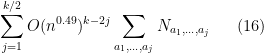
The expression (16) can then be bounded by

$\displaystyle 2^k \sum_{j=1}^{k/2} O(n^{0.49})^{k-2j} k^{O(k-2j) + O(1)} n^{\max(j+1, k/2)} \sum_{a_1,\ldots,a_j} 1.$

When ${j}$ is exactly ${k/2}$ , then all the ${a_1,\ldots,a_j}$ must equal ${2}$ , and so the contribution of this case simplifies to ${2^k k^{O(1)} n^{k/2}}$ . For ${j < k/2}$ , the numbers ${a_1-2,\ldots,a_j-2}$ are non-negative and add up to ${k-2j}$ , and so the total number of possible values for these numbers (for fixed ${j}$ ) can be bounded crudely by ${j^{k-2j} \leq k^{k-2j}}$ (for instance). Putting all this together, we can bound (16) by

$\displaystyle 2^k [ k^{O(1)} n^{k/2} + \sum_{j=1}^{k/2-1} O(n^{0.49})^{k-2j} k^{O(k-2j) + O(1)} n^{j+1} k^{k-2j} ]$

which simplifies by the geometric series formula (and the hypothesis ${k = O(\log^2 n)}$ ) to

$\displaystyle O( 2^k k^{O(1)} n^{k/2 + 0.98} )$

as required. $\Box$
We can use this to conclude the following matching upper bound to Proposition 32, due to Bai and Yin:

Theorem 36 (Weak Bai-Yin theorem, upper bound) Let ${M = (\xi_{ij})_{1 \leq i,j \leq n}}$ be a real symmetric matrix whose entries all have the same distribution ${\xi}$ , with mean zero, variance one, and fourth moment ${O(1)}$ . Then for every ${\varepsilon > 0}$ independent of ${n}$ , one has ${\|M\|_{op} \leq (2+\varepsilon) \sqrt{n}}$ asymptotically almost surely. In particular, ${\|M\|_{op} \leq (2+o(1))\sqrt{n}}$ asymptotically almost surely; as another consequence, the median of ${\|M\|_{op}}$ is at most ${(2+o(1))\sqrt{n}}$ . (If ${\xi}$ is bounded, we see in particular from Proposition 32 that the median is in fact equal to ${(2+o(1))\sqrt{n}}$ .)

The fourth moment hypothesis is best possible, as seen in the discussion after Theorem 12. We will discuss some generalisations and improvements of this theorem in other directions below.
Proof: To obtain Theorem 36 from Theorem 34 we use the truncation method. We split each ${\xi_{ij}}$ as ${\xi_{ij,\leq n^{0.49}} + \xi_{ij,>n^{0.49}}}$ in the usual manner, and split ${M = M_{\leq n^{0.49}} + M_{>n^{0.49}}}$ accordingly. We would like to apply Theorem 34 to ${M_{\leq n^{0.49}}}$ , but unfortunately the truncation causes some slight adjustment to the mean and variance of the ${\xi_{ij,\leq n^{0.49}}}$ . The variance is not much of a problem; since ${\xi_{ij}}$ had variance ${1}$ , it is clear that ${\xi_{ij,\leq n^{0.49}}}$ has variance at most ${1}$ , and it is easy to see that reducing the variance only serves to improve the bound (15). As for the mean, we use the mean zero nature of ${\xi_{ij}}$ to write

$\displaystyle {\bf E} \xi_{ij,\leq n^{0.49}} = - {\bf E} \xi_{ij,> n^{0.49}}.$

To control the right-hand side, we use the trivial inequality ${|\xi_{ij,\leq n^{0.49}}| \leq n^{- 3\times 0.49} |\xi_{ij}|^4}$ and the bounded fourth moment hypothesis to conclude that

$\displaystyle {\bf E} \xi_{ij,\leq n^{0.49}} = O( n^{-1.47} ).$

Thus we can write ${M_{\leq n^{0.49}} = \tilde M_{\leq n^{0.49}} + {\bf E} M_{\leq n^{0.49}}}$ , where ${\tilde M_{\leq n^{0.49}}}$ is the random matrix with coefficients

$\displaystyle \tilde \xi_{ij,\leq n^{0.49}} := \xi_{ij,\leq n^{0.49}} - {\bf E} \xi_{ij,\leq n^{0.49}}$

and ${{\bf E} M_{\leq n^{0.49}}}$ is a matrix whose entries have magnitude ${O(n^{-1.47})}$ . In particular, by Schur’s test this matrix has operator norm ${O(n^{-0.47})}$ , and so by the triangle inequality

$\displaystyle \|M\|_{op} \leq \| \tilde M_{\leq n^{0.49}} \|_{op} + \| M_{>n^{0.49}}\|_{op} + O( n^{-0.47} ).$

The error term ${O(n^{-0.47})}$ is clearly negligible for ${n}$ large, and it will suffice to show that

$\displaystyle \| \tilde M_{\leq n^{0.49}} \|_{op} \leq (2+\varepsilon/3) \sqrt{n} \ \ \ \ \ (19)$

and

$\displaystyle \| M_{> n^{0.49}} \|_{op} \leq \frac{\varepsilon}{3} \sqrt{n} \ \ \ \ \ (20)$

asymptotically almost surely.
We first show (19). We can now apply Theorem 34 to conclude that

$\displaystyle {\bf E} \| \tilde M_{\leq n^{0.49}} \|_{op}^k \leq (2+o(1))^k n^{k/2+1}$

for any ${k = O(\log^2 n)}$ . In particular, we see from Markov’s inequality that (19) holds with probability at most

$\displaystyle (\frac{2+o(1)}{2+\varepsilon/3})^k n.$

Setting ${k}$ to be a large enough multiple of ${\log n}$ (depending on ${\varepsilon}$ ), we thus see that this event (19) indeed holds asymptotically almost surely (indeed, one can ensure it happens with overwhelming probability, by letting ${k/\log n}$ grow slowly to infinity).
Now we turn to (20). The idea here is to exploit the sparseness of the matrix ${M_{> n^{0.49}}}$ . First let us dispose of the event that one of the entries ${\xi_{ij}}$ has magnitude larger than ${\frac{\varepsilon}{3} \sqrt{n}}$ (which would certainly cause (20) to fail). By the union bound, the probability of this event is at most

$\displaystyle n^2 {\bf P}(|\xi| \geq \frac{\varepsilon}{3} \sqrt{n}).$

By the fourth moment bound on ${\xi}$ and dominated convergence, this expression goes to zero as ${n \rightarrow \infty}$ . Thus, asymptotically almost surely, all entries are less than ${\frac{\varepsilon}{3} \sqrt{n}}$ .
Now let us see how many non-zero entries there are in ${M_{>n^{0.49}}}$ . By Markov’s inequality and the fourth moment hypothesis, each entry has a probability ${O( n^{- 4 \times 0.49} ) = O( n^{-1.96} )}$ of being non-zero; by the first moment method, we see that the expected number of entries is ${O( n^{0.04} )}$ . As this is much less than ${n}$ , we expect it to be unlikely that any row or column has more than one entry. Indeed, from the union bound and independence, we see that the probability that any given row and column has at least two non-zero entries is at most

$\displaystyle n^2 \times O( n^{-1.96})^2 = O( n^{-1.92} )$

and so by the union bound again, we see that with probability at least ${1-O(n^{-0.92})}$ (and in particular, asymptotically almost surely), none of the rows or columns have more than one non-zero entry. As the entries have magnitude at most ${\frac{\varepsilon}{3} \sqrt{n}}$ , the bound (20) now follows from Schur’s test, and the claim follows. $\Box$
We can upgrade the asymptotic almost sure bound to almost sure boundedness:

Theorem 37 (Strong Bai-Yin theorem, upper bound) Let ${\xi}$ be a real random variable with mean zero, variance ${1}$ , and finite fourth moment, and for all ${1 \leq i \leq j}$ , let ${\xi_{ij}}$ be an iid sequence with distribution ${\xi}$ , and set ${\xi_{ji} := \xi_{ij}}$ . Let ${M_n := (\xi_{ij})_{1 \leq i,j \leq n}}$ be the random matrix formed by the top left ${n \times n}$ block. Then almost surely one has ${\limsup_{n \rightarrow \infty} \|M_n\|_{op}/\sqrt{n} \leq 2}$ .

Exercise 38 By combining the above results with Proposition 32 and Exercise 15, show that with the hypotheses of Theorem 37 with ${\xi}$ bounded, one has ${\lim_{n \rightarrow \infty} \|M_n\|_{op}/\sqrt{n} =2}$ almost surely. (The same claim is true without the boundedness hypothesis; we will see this in the next set of notes, after we establish the semicircle law.)

Proof: We first give ourselves an epsilon of room. It suffices to show that for each ${\varepsilon > 0}$ , one has

$\displaystyle \limsup_{n \rightarrow \infty} \|M_n\|_{op}/\sqrt{n} \leq 2+\varepsilon \ \ \ \ \ (21)$

almost surely.
Next, we perform dyadic sparsification (as was done in the proof of the strong law of large numbers in Notes 1). Observe that any minor of a matrix has its operator norm bounded by that of the larger matrix; and so ${\|M_n\|_{op}}$ is increasing in ${n}$ . Because of this, it will suffice to show (21) almost surely for ${n}$ restricted to a lacunary sequence, such as ${n = n_m := \lfloor (1+\varepsilon)^m \rfloor}$ for ${m=1,2,\ldots}$ , as the general case then follows by rounding ${n}$ upwards to the nearest ${n_m}$ (and adjusting ${\varepsilon}$ a little bit as necessary).
Once we sparsified, it is now safe to apply the Borel-Cantelli lemma (Exercise 1 of Notes 0), and it will suffice to show that

$\displaystyle \sum_{m=1}^\infty {\bf P}( \|M_{n_m}\|_{op} \geq (2+\varepsilon) \sqrt{n_m} ) < \infty.$

To bound the probabilities ${{\bf P}( \|M_{n_m}\|_{op} \geq (2+\varepsilon) \sqrt{n_m})}$ , we inspect the proof of Theorem 36. Most of the contributions to this probability decay polynomially in ${n_m}$ (i.e. are of the form ${O(n_m^{-c})}$ for some ${c>0}$ ) and so are summable. The only contribution which can cause difficulty is the contribution of the event that one of the entries of ${M_{n_m}}$ exceeds ${\frac{\varepsilon}{3} \sqrt{n_m}}$ in magnitude; this event was bounded by

$\displaystyle n_m^2 {\bf P}(|\xi| \geq \frac{\varepsilon}{3} \sqrt{n_m}).$

But if one sums over ${m}$ using Fubini’s theorem and the geometric series formula, we see that this expression is bounded by ${O_\varepsilon({\bf E} |\xi|^4)}$ , which is finite by hypothesis, and the claim follows. $\Box$
Now we discuss some variants and generalisations of the Bai-Yin result.
Firstly, we note that the results stated above require the diagonal and off-diagonal terms to have the same distribution. This is not the case for important ensembles such as the Gaussian Orthogonal Ensemble (GOE), in which the diagonal entries have twice as much variance as the off-diagonal ones. But this can easily be handled by considering the diagonal separately. For instance, consider a diagonal matrix ${D = \hbox{diag}(\xi_{11},\ldots,\xi_{nn})}$ where the ${\xi_{ii} \equiv \xi}$ are identically distributed with finite second moment. The operator norm of this matrix is just ${\sup_{1 \leq i \leq n} |\xi_{ii}|}$ , and so by the union bound

$\displaystyle {\bf P}(\|D\|_{op} > \varepsilon \sqrt{n}) \leq n {\bf P}(|\xi| > \varepsilon \sqrt{n}).$

From the finite second moment and dominated convergence, the right-hand side is ${o_\varepsilon(1)}$ , and so we conclude that for for every fixed ${\varepsilon > 0}$ , ${\|D\|_{op} \leq \varepsilon \sqrt{n}}$ asymptotically almost surely; diagonalising, we conclude that ${\|D\|_{op} = o(\sqrt{n})}$ asymptotically almost surely. Because of this and the triangle inequality, we can modify the diagonal by any amount with identical distribution and bounded second moment (a similar argument also works for non-identical distributions if one has uniform control of some moment beyond the second, such as the fourth moment) while only affecting all operator norms by ${o(\sqrt{n})}$ .

Exercise 39 Modify this observation to extend the weak and strong Bai-Yin theorems to the case where the diagonal entries are allowed to have different distribution than the off-diagonal terms, and need not be independent of each other or of the off-diagonal terms, but have uniformly bounded fourth moment.

Secondly, it is a routine matter to generalise the Bai-Yin result from real symmetric matrices to Hermitian matrices, basically for the same reasons that Exercise 30 works. We leave the details to the interested reader.
The Bai-Yin results also hold for iid random matrices, where ${\xi_{ij} \equiv \xi}$ has mean zero, unit variance, and bounded fourth moment; this is a result of Yin, Bai, and Krishnaiah. Because of the lack of symmetry, the eigenvalues need not be real, and the bounds (9) no longer apply. However, there is a substitute, namely the bound

$\displaystyle \| M \|_{op}^k \leq \hbox{tr}((MM^*)^{k/2}) \leq n \|M\|_{op}^k, \ \ \ \ \ (22)$

valid for any ${n \times n}$ matrix ${M}$ with complex entries and every even positive integer ${k}$ .

Exercise 40 Prove (22).

It is possible to adapt all of the above moment calculations for ${\hbox{tr}(M^k)}$ in the symmetric or Hermitian cases to give analogous results for ${\hbox{tr}((MM^*)^{k/2})}$ in the non-symmetric cases; we do not give the details here, but mention that the cycles now go back and forth along a bipartite graph with ${n}$ vertices in each class, rather than in the complete graph on ${n}$ vertices, although this ends up not to affect the enumerative combinatorics significantly. Another way of viewing this is through the simple observation that the operator norm of a non-symmetric matrix ${M}$ is equal to the operator norm of the augmented matrix

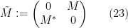
$\displaystyle \tilde M := \begin{pmatrix} 0 & M \\ M^* & 0 \end{pmatrix} \ \ \ \ \ (23)$

which is a ${2n \times 2n}$ Hermitian matrix. Thus one can to some extent identify an ${n \times n}$ iid matrix ${M}$ with a ${2n \times 2n}$ Wigner-type matrix ${\tilde M}$ , in which two ${n \times n}$ blocks of that matrix are set to zero.

Exercise 41 If ${M}$ has singular values ${\sigma_1,\ldots,\sigma_n}$ , show that ${\tilde M}$ has eigenvalues ${\pm \sigma_1,\ldots,\pm \sigma_n}$ . This suggests that the theory of the singular values of an iid matrix should resemble to some extent the theory of eigenvalues of a Wigner matrix; we will see several examples of this phenomenon in later notes.

When one assumes more moment conditions on ${\xi}$ than bounded fourth moment, one can obtain substantially more precise asymptotics on ${\hbox{tr}(M^k)}$ than given by results such as Theorem 34, particularly if one also assumes that the underlying random variable ${\xi}$ is symmetric (i.e. ${\xi \equiv -\xi}$ ). At a practical level, the advantage of symmetry is that it allows one to assume that the high-multiplicity edges in a cycle are traversed an even number of times; see the following exercise.

Exercise 42 Let ${X}$ be a bounded real random variable. Show that ${X}$ is symmetric if and only if ${{\bf E} X^k=0}$ for all positive odd integers ${k}$ .
Next, extend the previous result to the case when ${X}$ is subgaussian rather than bounded. (Hint: The slickest way to do this is via the characteristic function ${e^{itX}}$ and analytic continuation; it is also instructive to find a “real-variable” proof that avoids the use of this function.)

By using these methods, it is in fact possible to show that under various hypotheses, ${\|M\|_{op}}$ is concentrated in the range ${[2\sqrt{n}-O(n^{-1/6}), 2\sqrt{n}+O(n^{-1/6})]}$ , and even to get a universal distribution for the normalised expression ${(\|M\|_{op}-2\sqrt{n}) n^{1/6}}$ , known as the Tracy-Widom law. See this paper of Soshnikov for details. There has also been a number of subsequent variants and refinements of this result (as well as counterexamples when not enough moment hypotheses are assumed); see for instance these papers of Soshnikov, Soshnikov-Fyodorov, Ruzmaikina, Péché, Vu, Soshnikov-Péché, Péché, Khorunzhiy and Tao-Vu for an (incomplete) sample of the work in this area. (Similar results for some non-independent distributions are also available, see e.g. this paper of Deift and Gioev, which (like many of the other references just cited) builds upon the original work of Tracy and Widom that handled special ensembles such as GOE and GUE.)

61 comments

Comments feed for this article

10 January, 2010 at 8:17 am

Mark Meckes

Regarding the end of Remark 4, if you’ll forgive the immodesty, in this paper, I showed that one can get better concentration results for eigenvalues of symmetric matrices than Alon, Krivelevich, and Vu, by using actually the same version of Talagrand’s inequality you quoted previously (i.e. the more abstract version used by AKV is not necessary here).

10 January, 2010 at 9:12 am

Terence Tao

Thanks for the reference! I’ve updated the remark accordingly.

10 January, 2010 at 11:22 am

Mark Meckes

By the way, this post is by far the pedagogically nicest presentation I’ve ever seen of the moment method for random matrices. Beautiful!

10 January, 2010 at 3:43 pm

Paul Leopardi

Nice notes. I haven’t worked through them yet, but it looks like they would apply to the symmetric Wigner case where the diagonal entries are constant and the upper triangle is iid N(0,1), or iid with mean 0, variance 1 and bounded values: “Typically, the strictly upper triangular coefficients will be iid, as will the diagonal coefficients, but the two classes of coefficients may have a different distribution”. Working through the notes would then help me understand the moments of the Gram matrices for polynomial interpolation on the sphere.
Best, Paul

12 January, 2010 at 9:03 pm

254A, Notes 3a: Eigenvalues and sums of Hermitian matrices « What’s new

[…] values of non-Hermitian matrices (which is consistent with the discussion near Exercise 16 of Notes 3). However, the situation is markedly different when dealing with eigenvalues of non-Hermitian […]

13 January, 2010 at 4:29 am

Orr

I am having trouble understanding Lemma 1 and its proof:
Exercise 4, Exercise 5, or Theorem 9 from Notes 1 that you use do not have $n$ appearing on the right hand side, so it is not clear how you get the $n$ in $exp(-cAn)$ .
And in the claim that $|X_i \cdot x| \geq A$ occurs with probability at most $exp(-cAn)$ seems inappropriate that there should be dependence on $n$ . For instance, if the entries of the matrix are iid and taking $x = 1/ \sqrt{n} (1,1,\ldots,1)$ , the probability of the event $|X_i \cdot x| \geq A$ converges to the probability that a Gaussian is greater than $A$, and that should remain bounded from below.

13 January, 2010 at 9:28 am

Terence Tao

Oops, you’re right, this is not the correct argument. I’ve replaced it with one which should be more correct (and which only holds for A sufficiently large, as it should.)

24 January, 2010 at 6:15 pm

Steven Heilman

Some minor typos?

1. Proof of Corollary 4: “…from Lemma 3, \Sigma [h]as cardinality…”

2. Section 2: “Suppose now that M={…} [is] a matrix”

3. After Exercise 4: Application of Jensen’s, needs \geq

4. Section 4, after (12): application of Markov’s inequality has extraneous E symbol?: “and thus by Markov’s inequality…”

{{\bf E} \hbox{tr}(M^4) \leq O_\epsilon(n^3)}

5. Beginning of Section 5: Now let [us?] consider…

6. Section 5, Example 1: If I’m not mistaken, the partition (a,b,c,d,b,c) is crossing. I think you meant (a,b,c,d,c,b), since this has the combinatorial label specified in the Proof of Lemma 9?

7. Is there any known connection between the expected operator norm of a random matrix and the projection constant of a finite dimensional Banach space? Maybe it is only vaguely related, but \lambda(X)\leq\sqrt{dim X} holds, where \lambda(X) is the projection constant of a Banach space X.

8. Near end of proof of Theorem 14: “each entry has a probability … probability[sic]”

30 January, 2010 at 9:57 pm

Anand Rajagopalan

Hi Professor,

Great notes!
A couple of minor typos:
-The occurrence of (a,b,c,d,b,c) in the proof of lemma 9 should be (a,b,c,d,c,b).
-The first inequality in section 6 should be reversed I think.

[Corrected, thanks – T.]

2 February, 2010 at 1:33 pm

254A, Notes 4: The semi-circular law « What’s new

[…] results in random matrix theory, namely the Wigner semi-circle law for Wigner matrices. Recall from previous notes that a Wigner Hermitian matrix ensemble is a random matrix ensemble of Hermitian matrices (thus ; […]

10 February, 2010 at 10:56 pm

245A, Notes 5: Free probability « What’s new

[…] a complex number). As before, we see that is a -linear functional that maps to . As we saw in Notes 3, the moment method for random matrices is based on a computation of the moments […]

5 March, 2010 at 1:47 pm

254A, Notes 7: The least singular value « What’s new

[…] the “soft edge” of the spectrum, that was discussed back in Notes 3, so one may at first think that the methods that were effective in controlling the latter, namely […]

14 March, 2010 at 11:33 am

254A, Notes 8: The circular law « What’s new

[…] the origin. Indeed, for iid matrices with subgaussian entries, one can show (using the methods from Notes 3) that the operator norm of is almost surely; this, combined with (2) and Laurent expansion, tells […]

31 March, 2010 at 9:24 am

PDEbeginner

Dear Prof. Tao,

I have some problems on how to estimate the median by the moments:

1. Ex 8: I don’t see how to obtain that the median of $||M||_{op}$ is at least $(5^{1/6}+o(1)) \sqrt{n}$ from the bounds therein and the assumption $K=O(1)$ .

2. Argument immediately above Prop 8: I understood the estimate of sixth moments and that by Markov inequality, but didn’t know how to get the median estimate.

My questions are most probably very trivial, it would be very appreciated if you could give some hints.

31 March, 2010 at 10:11 am

Terence Tao

For exercise 8, use concentration of measure (Prop 7) to extract information about the median from the fourth moment.

For the second argument: if ${\bf P}( \|M\|_{op} > \lambda ) < 1/2$ , then the median of $\|M\|_{op}$ is necessarily at most $\lambda$ .

1 April, 2010 at 9:28 am

PDEbeginner

Dear Prof. Tao,

Thanks a lot for your help!

I think I got it. I think the condition $K=O(1)$ is for applying Talagrand’s inequality.

As for the Talagrand’s inequality in note 1, I would like to give an immature suggestion (maybe it is wrong):

It seems that the $1$ -Lipschitz condition is a little confusing. At the first glance, one might think that the Talagrand’s inequality holds only when Lipschitz constant of $F$ is 1. After checking the proof, I think we only need that Lipschitz constant is bounded. So I think it could be better to add some remark near the Talagrand’s Theorem (if I am right).

31 March, 2010 at 9:26 am

PDEbeginner

sorry, the problem 2 is $k$ -th moment.

23 May, 2010 at 8:28 am

Anonymous

I have one question. Close to the end of this note, there is “From the finite second moment and dominated convergence, the right hand side is o_{\epsilon}(1)”.

I used the markov inequality to see that actually that right hand side is bounded by a constant, rather than o_{\epsilon}(1)”.

Could you expand on this argument? Thank you very much.

a typo: before “we inspect the proof of Theorem 14″, a right bracket is missing.

23 May, 2010 at 11:07 am

Terence Tao

From dominated convergence, ${\bf E}(\lambda^2 {\bf I}( |\xi| \geq \lambda ) )$ goes to zero as $\lambda \to \infty$ , if ${\bf E} |\xi|^2$ is finite.

15 November, 2010 at 2:52 am

Guillaume

Dear Prof. Tao,

Unless I missed something, there appears to be a misprint in Lemma 9 (and at several subsequent places), the product should be $n(n-1)\cdots (n-k/2)$ instead of $n(n-1)\cdots (n-k/2-1)$ …

[Corrected, thanks – T.]

20 November, 2010 at 11:19 pm

Dai

Dear Prof. Tao,

At the end of section 4, you said “How many different classes could there be? We have to assign up to $k/2$ labels to $k$ edges, so a crude upper bound here is $k^{k/2}$ .”

Why this is true? I think by this argument the crude upper bound should be $(k/2)^k$ . Maybe this problem is trivial for you. Thank you very much in advance.

[Oops, this was a typo (which unfortunately propagated throughout the section. Fixed now, – T.]

10 April, 2013 at 4:22 pm

Mustafa Said

Terry,
In the symmetrisation inequality (4), I think one can find an upper bound on the operator norm of the right hand side since when you introduce the random sign matrix E, it acts as an operator on M. There is a paper, “Restricted Schur Multipliers and their Applications,” by Timur Oikhberg that may help on this end.

4 November, 2013 at 1:48 pm

Real stable polynomials and the Kadison-Singer problem | What's new

[…] be, one might first try to compute the expected operator norm and then apply Proposition 1; see this previous blog post for examples of this strategy (and related strategies, based on comparing with more tractable […]

24 November, 2013 at 12:25 pm

Relatings turings use of norm (statistics) to eigenvalues | Peter's ruminations

[…] https://terrytao.wordpress.com/2010/01/09/254a-notes-3-the-operator-norm-of-a-random-matrix/ […]

5 August, 2014 at 2:57 pm

Yash Deshpande

A question regarding the estimate for $N_{a_1, a_2 \dots a_j}$ :
while recording the data for reconstructing the cycle $i_1 \dots i_k$ , it appears to me that one would need the end point of each non-innovative leg. This can be recorded using (for instance) the position of the innovative leg that first visited that vertex and incurs additional $k^m$ entropy cost. This does not change significantly the bound, in particular the estimate used ultimately is correct even with this modification.

[Corrected, thanks – T.]

29 October, 2014 at 10:28 am

Marwin Mayer

Dear Prof. Tao,

I have a problem understanding a proof. (Here it is Proposition 11). You say “[…] we can combine this with Exercise 5 to conclude that the median (or mean) of {\|M\|_{op}} is at least {(C_{k/2}^{1/k}+o_k(1)) \sqrt{n}}”. But how can you use exercise 5 to conclude that?

Sincerely yours,

Marwin Mayer

29 October, 2014 at 10:42 am

Terence Tao

If the median of $\|M\|_{op}$ was less than $(C_{k/2}-\varepsilon)^{1/k} \sqrt{n}$ for some fixed $\varepsilon > 0$ , then by using Exercise 5 one would have $\|M\|_{op}$ bounded by $(C_{k/2}-\varepsilon/2)^{1/k} \sqrt{n}$ with overwhelming probability. One could then obtain an upper bound on the k^th moment that was of the form $(C_{k/2}-\varepsilon/2+o(1)) n^{k/2}$ , contradicting the lower bound on this moment.

30 October, 2014 at 7:13 am

Marwin Mayer

Thank you very much! Now I understand it.

26 February, 2015 at 8:06 pm

elegantrium

Hi Dear Prof. Tao,
Is there any sharp result on the concentration inequality for schatten norm of a random matrix, where the Schatten norm is defined as in http://en.wikipedia.org/wiki/Schatten_norm?

Sincerely yours,
Jason

26 February, 2015 at 10:16 pm

Terence Tao

I would have a look at the article of Meckes http://www.ams.org/mathscinet-getitem?mr=2057479 (which considers general convex norms of random matrices).

23 October, 2015 at 8:06 am

275A, Notes 3: The weak and strong law of large numbers | What's new

[…] can obtain much sharper information on quantities such as the operator norm of a random matrix; see this previous blog post for further […]

17 November, 2015 at 11:27 pm

Canyi

Dear Prof. Tao,

It is known that for a matrix $A\in\mathbb{R}^{n\times n}$ which is i.i.d., its spectral norm $||A||\leq C\sqrt{n}$ .

Now, I have a related and interesting about the spectral norm of the block circulant matrix defined as

$\displaystyle A= \begin{bmatrix} A_{1} &A_{m} &\cdots &A_{2} \\ A_{2} &A_{1} & \cdots &A_{3} \\ \vdots & \vdots & \ddots & \vdots \\ A_{m} & A_{m-1} & \cdots & A_{1} \end{bmatrix} \in\mathbb{R}^{nm\times nm}.$

where each $A_i\in\mathbb{R}^{n\times n}$ is an i.i.d. matrix, and its elements have the distribution

$[A_i]_{a,b} = \begin{cases} 1, & \text{w.p. } \rho/2, \\ 0, & \text{w.p. } 1-\rho,\\ -1, & \text{w.p. } \rho/2. \end{cases}$

for some $0<\rho<1$ .

Can we prove that $\|A\| \leq C\sqrt{nm}$ for some constant $C$ with large probability?

18 November, 2015 at 8:33 am

Terence Tao

I expect that this should be provable by several of the methods in this post (e.g. I believe the moment method will eventually work, although the combinatorics are messy). There may be a more elegant approach using more advanced matrix inequalities (e.g. noncommutative Khinchin) or free probability methods, but I don’t immediately see such an argument.

6 February, 2016 at 3:24 pm

Hi Prof. Tao,

The covering method gives a guarantee with probability 1-exp(-Omega(n)).
Can’t one get a similar probability bound in the trace power method by using
polynomial concentration results?

7 February, 2016 at 4:52 pm

Terence Tao

In principle yes, but one would have to apply concentration of measure results to polynomials of degree about $O(\log n)$ , so one has to be careful regarding how the constants depend on degree. (But if one was content with an upper bound of the form $O_{\varepsilon}(n^{1/2+\varepsilon})$ rather than $O(n^{1/2})$ then one could work with polynomials of degree $O(1)$ , in which case standard concentration of measure results would work without difficulty.)

3 July, 2016 at 2:03 am

Dear Prof. Tao;
Would you please give me a hint on Exercise 1?
Thanks.

[Adapt the volume packing arguments used to prove Lemma 3. -T.]

3 July, 2016 at 9:48 am

OK, Thank you!

21 November, 2016 at 9:37 pm

Anonymous

Dear Prof. Tao,
I have a question. For a matrix $A\in R^{n\times n}$ whose entries obey

$A_{ij} = \begin{cases} 1, & \text{w.p.} \ 1/2, \\ -1, & \text{w.p.} \ 1/2, \end{cases}$

we have $\|A\|_{op}\leq c\sqrt{n}$ .

Now my question is that for a matrix $A\in R^{n\times n}$ whose entries obey

$A_{ij} = \begin{cases} 1, & \text{w.p.} \ \rho/2, \\ 0, & \text{w.p.} \ 1-\rho, \\ -1, & \text{w.p.} \ \rho/2, \end{cases}$

how could we prove $\|A\|_{op}\leq c\sqrt{\rho n}$ (this conclusion is right, but I do not know how to prove it)? Thanks a lot!

10 January, 2017 at 2:32 am

Anonymous

Minor typo in Lemma 3: the sphere in the lemma should be n-dimensional, should it not?

[Corrected, thanks – T.]

8 March, 2017 at 1:43 am

keej

I’m probably missing something simple, but I do not see why Exercise 7 requires $K = o(\sqrt{n})$ . Each term (12) ends up being nonnegative, so to lower bound the sum it suffices to consider only the terms in the “first case,” of which there are 2n(n-1)(n-2) and each has value 1. By (9) it suffices to divide this by n and take the fourth root, which yields $2^{1/4} (1 + o(1)) \sqrt{n}$ as desired.

Could someone who did this please help me out?

[Fair enough; but this positivity is a special feature of the fourth moment and would not be available for the analogous assertions for higher moments. -T]

28 March, 2017 at 9:53 pm

keej

I see, thanks for the clarification!

25 December, 2017 at 5:44 am

AL Ray

Regarding Remark 1, I think that $\lambda/(1-\epsilon)$ should actually be $\lambda (1-\epsilon)$ . I assume that the definition of 1/2-net coincides with \epsilon – net, in which case when plugging \epsilon = 1/2 we should be getting a factor of half and not 2.

[Corrected, thanks – T.]

6 January, 2018 at 9:15 pm

Anonymous

A typo: In proposition 7, $M\|M\|_{op}$ should be $\mathbf{M}\|M\|_{op}$ . [Corrected, thanks – T.]
A question: I really do not know how to prove that $C_{k/2} n(n-1)\cdots (n-k/2)=(C_{k/2}+o(1))n^{k/2+1}$ . Any hints?
Thanks!

6 January, 2018 at 9:41 pm

Anonymous

PS: The difficulty is that $k$ could be large if $n$ is large.

6 January, 2018 at 10:13 pm

Anonymous

PSS: I can only show that $C_{k/2}n(n-1))\cdots (n-k/2)=C_{k/2}(1+o(1))n^{k/2+1}$ .

7 January, 2018 at 12:12 am

Terence Tao

The decay rate in $o_k(1)$ is allowed to depend on $k$ (see the beginning of section 5).

7 January, 2018 at 6:10 pm

Anonymous

I am sorry, but I am concerned with the beginning of the proof of Theorem 12. There it is $o(1)$ but not $o_k(1)$. I don’t know how the independence on $k$ disappears, since $k=O(\log^2 n)$ could be very large when $n$ is large. Could you please have a check? Thanks!

15 January, 2018 at 3:21 am

Anonymous

Dear Terry,

In this post, you used the argument multiple times that
$n^2 {\bf P}(|\xi| \geq \frac{\epsilon}{3} \sqrt{n})$
goes to 0 when $n\rightarrow \infty$ due to the existence of ${\bf E}\xi^4$ . But Markov inequality will only give us $n^{-2}$ which is canceled by $n^2$ ahead. Do we need $4+\epsilon$ -th moment here? Or do I miss something?

Best,
Jeffrey

15 January, 2018 at 1:22 pm

Terence Tao

Apply dominated convergence to the random variables $n^2 1_{|\xi| \geq \frac{\epsilon}{3} \sqrt{n}}$ , which are pointwise dominated by $(\frac{3}{\epsilon})^4 |\xi|^4$ .

4 October, 2018 at 12:09 pm

Drew Brady

Is Prop 7 correct? I.e., Your argument shows that $\|A - B\|_{op} \leq \|(a_{ij}) - (b_{ij})\|$ , where the norm on the right hand side is the Euclidean norm on $\mathbf{C}^{2n}$ . Don’t you need, however that $|\|A\|_{op} - \|B\|_{op}| \leq \|A - B\|_{op}$ , in order for this argument to work out?

5 October, 2018 at 2:15 pm

Terence Tao

Yes, but this is immediate from the triangle inequality for the operator norm.

8 January, 2021 at 9:07 am

Tim

I have a question about Exercise 10. It seems that the cycle 1, 2, 1, 3, 1, 4, 1 (4 vertices, 6 edges) is a valid cycle to be counted, but it does not satisfy the condition in Exercise 10?

[Oops, there was an extra condition for the edges, now added. -T.]

14 January, 2021 at 3:08 pm

Anonymous

This is just a thought on the volume packing argument (Lemma 4). Each of the balls of radius $\epsilon/2$ centered points of the net accounts for some volume, but this volume in enclosed inside the larger ball of radius $3/2$ . So is the upper bound on the cardinality just the ratio of the volume of the larger ball over the volume of a ball of radius $\epsilon/2$ ?

14 March, 2021 at 1:32 pm

Anonymous

Dear Professor Tao,

Do you know of some recent papers where finer volume packing arguments are used for things such as the operator norm, condition number etc. I was curious to learn more about these arguments.

9 January, 2022 at 12:15 pm

Tom Copeland

Numerous occurrences in analysis, enumerative geometry, combinatorics, probability, and physics of the sequence of double factorials of odd numbers in Remark 31 are noted in https://oeis.org/A001147 and refs therein, as well as associations to other number sequences, such as the Catalans. For the benefit of others, it would be nice to ref this post in the OEIS entry.

15 June, 2022 at 1:36 am

Aurelien

Very minor comment: In Lemma 1 in the RHS, shouldn’t A be squared? (as a result of applying Markov’s inequality)

[Corrected, thanks – T.]

17 March, 2024 at 5:13 pm

Anonymous

Dear Professor Tao,

I am very confused about the bound before weak Bai-Yin theorem, you said that

by the geometric series formula (and the hypothesis ${k = O(log^2 n)}$ ), we can get the following bound, here I have two questions. The first is that the geometric series doesn’t converge here and the bound I get is of the form O(2^kk^O(1)n^0.99k) and I can’t get rid of the 0.49k. The second is I’m not sure how to use the log bound for k. I would appreciate it very much if you could bother to answer it. Thanks a lot!

displaystyle O( 2^k k^{O(1)} n^{k/2 + 0.98} )

30 March, 2024 at 6:22 pm

Anonymous

I’m not sure if I’m following the use of Markov’s inequality in lemma 2.3.1. We have that $E[e^{c|Mx|^{2}}] \leq C^{n}$ . My understanding of the application of Markov’s inequality is as follows:

$P[ |Mx| \geq A\sqrt{n} ] = P[ e^{c|Mx|^{2}} \geq e^{c(A\sqrt{n})^{2}} \leq C^{n} e^{-c(A\sqrt{n})^{2}}$

I must be doing something wrong?

31 March, 2024 at 6:25 am

Anonymous

Nevermind, I think the constants are different in the proof and in the statement.

31 March, 2024 at 12:40 pm

Anonymous

Dear Professor Tao,

I’m very confused about the bound before the weak Bai-Yin theorem. You said that by the geometric series formula and $k=O(log^2n)$ , we can get the bound $O(2^kk^{O(1)}n^{k/2+0.98})$ . My question is that the geometric series doesn’t converge here and the bound I get is of the form $O(2^kk^{O(1)}n^{0.99k})$ . I would appreciate it very much if you could bother to answer it. Thanks a lot!

[The dominant term here is when $j = k/2-1$ , which gives the $O(2^kk^{O(1)}n^{k/2+0.98})$ bound; the other terms decay at an exponential rate away from this value. -T]

	Anonymous on Erratum for “An inverse…
	Anonymous on Erratum for “An inverse…
	Anonymous on Pointwise ergodic theorems for…
	Anonymous on 275A, Notes 3: The weak and st…
	Terence Tao on Pointwise ergodic theorems for…
	Terence Tao on Erratum for “An inverse…
	Anonymous on Notes on the B+B+t theore…
	Anonymous on Pointwise ergodic theorems for…
	Anonymous on Erratum for “An inverse…
	Erratum for “A… on An inverse theorem for the Gow…
	Anonymous on Analysis II
	Anonymous on Notes on the B+B+t theore…
	Anonymous on Twisted convolution and the se…
	Anonymous on A generalized Cauchy-Schwarz i…
	Notes on the B+B+t t… on Ultrafilters, nonstandard anal…

254A, Notes 3: The operator norm of a random matrix

Recent Comments

Articles by others

Diversions

Mathematics

Selected articles

Software

The sciences

Top Posts

Archives

Categories

The Polymath Blog

61 comments

Leave a comment Cancel reply

For commenters

254A, Notes 3: The operator norm of a random matrix

Share this:

Recent Comments

Articles by others

Diversions

Mathematics

Selected articles

Software

The sciences

Top Posts

Archives

Categories

The Polymath Blog

61 comments

Leave a comment Cancel reply

For commenters