
You are currently browsing the tag archive for the ‘finite time blowup’ tag.
Just a brief post to record some notable papers in my fields of interest that appeared on the arXiv recently.
- “A sharp square function estimate for the cone in
“, by Larry Guth, Hong Wang, and Ruixiang Zhang. This paper establishes an optimal (up to epsilon losses) square function estimate for the three-dimensional light cone that was essentially conjectured by Mockenhaupt, Seeger, and Sogge, which has a number of other consequences including Sogge’s local smoothing conjecture for the wave equation in two spatial dimensions, which in turn implies the (already known) Bochner-Riesz, restriction, and Kakeya conjectures in two dimensions. Interestingly, modern techniques such as polynomial partitioning and decoupling estimates are not used in this argument; instead, the authors mostly rely on an induction on scales argument and Kakeya type estimates. Many previous authors (including myself) were able to get weaker estimates of this type by an induction on scales method, but there were always significant inefficiencies in doing so; in particular knowing the sharp square function estimate at smaller scales did not imply the sharp square function estimate at the given larger scale. The authors here get around this issue by finding an even stronger estimate that implies the square function estimate, but behaves significantly better with respect to induction on scales.
- “On the Chowla and twin primes conjectures over
“, by Will Sawin and Mark Shusterman. This paper resolves a number of well known open conjectures in analytic number theory, such as the Chowla conjecture and the twin prime conjecture (in the strong form conjectured by Hardy and Littlewood), in the case of function fields where the field is a prime power
which is fixed (in contrast to a number of existing results in the “large
” limit) but has a large exponent
. The techniques here are orthogonal to those used in recent progress towards the Chowla conjecture over the integers (e.g., in this previous paper of mine); the starting point is an algebraic observation that in certain function fields, the Mobius function behaves like a quadratic Dirichlet character along certain arithmetic progressions. In principle, this reduces problems such as Chowla’s conjecture to problems about estimating sums of Dirichlet characters, for which more is known; but the task is still far from trivial.
- “Bounds for sets with no polynomial progressions“, by Sarah Peluse. This paper can be viewed as part of a larger project to obtain quantitative density Ramsey theorems of Szemeredi type. For instance, Gowers famously established a relatively good quantitative bound for Szemeredi’s theorem that all dense subsets of integers contain arbitrarily long arithmetic progressions
. The corresponding question for polynomial progressions
is considered more difficult for a number of reasons. One of them is that dilation invariance is lost; a dilation of an arithmetic progression is again an arithmetic progression, but a dilation of a polynomial progression will in general not be a polynomial progression with the same polynomials
. Another issue is that the ranges of the two parameters
are now at different scales. Peluse gets around these difficulties in the case when all the polynomials
, so that one can still run a density increment argument efficiently. To resolve the second difficulty one needs to find a quantitative concatenation theorem for Gowers uniformity norms. Many of these ideas were developed in previous papers of Peluse and Peluse-Prendiville in simpler settings.
- “On blow up for the energy super critical defocusing non linear Schrödinger equations“, by Frank Merle, Pierre Raphael, Igor Rodnianski, and Jeremie Szeftel. This paper (when combined with two companion papers) resolves a long-standing problem as to whether finite time blowup occurs for the defocusing supercritical nonlinear Schrödinger equation (at least in certain dimensions and nonlinearities). I had a previous paper establishing a result like this if one “cheated” by replacing the nonlinear Schrodinger equation by a system of such equations, but remarkably they are able to tackle the original equation itself without any such cheating. Given the very analogous situation with Navier-Stokes, where again one can create finite time blowup by “cheating” and modifying the equation, it does raise hope that finite time blowup for the incompressible Navier-Stokes and Euler equations can be established… In fact the connection may not just be at the level of analogy; a surprising key ingredient in the proofs here is the observation that a certain blowup ansatz for the nonlinear Schrodinger equation is governed by solutions to the (compressible) Euler equation, and finite time blowup examples for the latter can be used to construct finite time blowup examples for the former.
I’ve just posted to the arXiv my paper “Finite time blowup for Lagrangian modifications of the three-dimensional Euler equation“. This paper is loosely in the spirit of other recent papers of mine in which I explore how close one can get to supercritical PDE of physical interest (such as the Euler and Navier-Stokes equations), while still being able to rigorously demonstrate finite time blowup for at least some choices of initial data. Here, the PDE we are trying to get close to is the incompressible inviscid Euler equations


in three spatial dimensions, where 


where 


One can then generalise this system by replacing the operator 


For example, the surface quasi-geostrophic (SQG) equations can be written in this form, as discussed in this previous post. One can view 
The generalised Euler equations carry much of the same geometric structure as the true Euler equations. For instance, the transport equation 


The true Euler equations are suspected of admitting smooth localised solutions which blow up in finite time; there is now substantial numerical evidence for this blowup, but it has not been proven rigorously. The main purpose of this paper is to show that such finite time blowup can at least be established for certain generalised Euler equations that are somewhat close to the true Euler equations. This is similar in spirit to my previous paper on finite time blowup on averaged Navier-Stokes equations, with the main new feature here being that the modified equation continues to have a Lagrangian structure and a vorticity formulation, which was not the case with the averaged Navier-Stokes equation. On the other hand, the arguments here are not able to handle the presence of viscosity (basically because they rely crucially on the Kelvin circulation theorem, which is not available in the viscous case).
In fact, three different blowup constructions are presented (for three different choices of vector potential operator
The second blowup construction is based on a connection between the two-dimensional SQG equation and the three-dimensional generalised Euler equations, discussed in this previous post. Namely, any solution to the former can be lifted to a “two and a half-dimensional” solution to the latter, in which the velocity and vorticity are translation-invariant in the vertical direction (but the velocity is still allowed to contain vertical components, so the flow is not completely horizontal). The same embedding also works to lift solutions to generalised SQG equations in two dimensions to solutions to generalised Euler equations in three dimensions. Conveniently, even if the vector potential operator for the generalised SQG equation fails to be self-adjoint, one can ensure that the three-dimensional vector potential operator is self-adjoint. Using this trick, together with a two-dimensional version of the first blowup construction, one can then construct a generalised Euler equation in three dimensions with a vector potential that is both self-adjoint and positive definite, and still admits solutions that blow up in finite time, though now the blowup is now a vortex sheet creasing at on a line, rather than a vortex tube pinching at a point.
This eliminates the main defect of the first blowup construction, but introduces two others. Firstly, the blowup is less stable, as it relies crucially on the initial data being translation-invariant in the vertical direction. Secondly, the solution is not spatially localised in the vertical direction (though it can be viewed as a compactly supported solution on the manifold 

As with the previous papers in this series, these blowup constructions do not directly imply finite time blowup for the true Euler equations, but they do at least provide a barrier to establishing global regularity for these latter equations, in that one is forced to use some property of the true Euler equations that are not shared by these generalisations. They also suggest some possible blowup mechanisms for the true Euler equations (although unfortunately these mechanisms do not seem compatible with the addition of viscosity, so they do not seem to suggest a viable Navier-Stokes blowup mechanism).
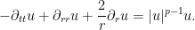
I’ve just uploaded to the arXiv my paper Finite time blowup for high dimensional nonlinear wave systems with bounded smooth nonlinearity, submitted to Comm. PDE. This paper is in the same spirit as (though not directly related to) my previous paper on finite time blowup of supercritical NLW systems, and was inspired by a question posed to me some time ago by Jeffrey Rauch. Here, instead of looking at supercritical equations, we look at an extremely subcritical equation, namely a system of the form

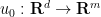
where 


for a scalar field 

We do not assume any Hamiltonian structure, so we do not require 


which (from the assumption that 

One might expect that one could keep iterating this and obtain a priori bounds on 


and

ensure that the map 


where there is a troublesome lower order term of size 


In medium dimensions, it is possible to use dispersive estimates for the wave equation (such as the famous Strichartz estimates) to overcome these problems. This line of inquiry was pursued (albeit for slightly different classes of nonlinearity 
In my paper, I complement these positive results with an almost matching negative result:
Theorem 1 If
and
, then there exists a nonlinearity
The construction crucially relies on the ability to choose the nonlinearity 


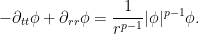
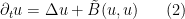
Let us first give some back-of-the-envelope calculations suggesting why there could be finite time blowup in eleven and higher dimensions. For sake of this discussion let us restrict attention to the sine-Gordon equation 


on 

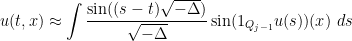
On 


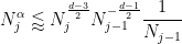
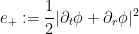
Next, when restricted to frequencies of order 

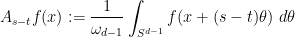
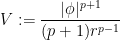
where 


on
Since 


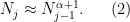
which when combined with our ansatz that
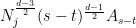
which on applying (2) gives the further constraint
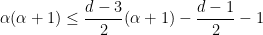
which can be rearranged as
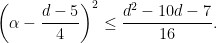
It is now clear that the optimal choice of 

and this blowup ansatz is only self-consistent when

or equivalently if
To turn this ansatz into an actual blowup example, we will construct 


for an arbitrary smooth function 

This precise and relatively simple formula for
It is not clear to me what to conjecture for 

…
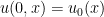
I’ve just uploaded to the arXiv my paper Finite time blowup for a supercritical defocusing nonlinear wave system, submitted to Analysis and PDE. This paper was inspired by a question asked of me by Sergiu Klainerman recently, regarding whether there were any analogues of my blowup example for Navier-Stokes type equations in the setting of nonlinear wave equations.
Recall that the defocusing nonlinear wave (NLW) equation reads

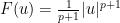
where 
where 


Formally, solutions to the equation (2) enjoy a conserved energy
![\displaystyle E[u] = \int_{{\bf R}^d} \frac{1}{2} \|\partial_t u \|^2 + \frac{1}{2} \| \nabla_x u \|^2 + F(u)\ dx.](https://s0.wp.com/latex.php?latex=%5Cdisplaystyle+E%5Bu%5D+%3D+%5Cint_%7B%7B%5Cbf+R%7D%5Ed%7D+%5Cfrac%7B1%7D%7B2%7D+%5C%7C%5Cpartial_t+u+%5C%7C%5E2+%2B+%5Cfrac%7B1%7D%7B2%7D+%5C%7C+%5Cnabla_x+u+%5C%7C%5E2+%2B+F%28u%29%5C+dx.&bg=ffffff&fg=000000&s=0&c=20201002)
Using this conserved energy, it is possible to establish global regularity for the Cauchy problem (2) in the energy-subcritical case when 


![\displaystyle \int_0^T \int_{{\bf R}^d} \frac{|u(t,x)|^{p+1}}{|x|}\ dx dt \lesssim E[u]](https://s0.wp.com/latex.php?latex=%5Cdisplaystyle+%5Cint_0%5ET+%5Cint_%7B%7B%5Cbf+R%7D%5Ed%7D+%5Cfrac%7B%7Cu%28t%2Cx%29%7C%5E%7Bp%2B1%7D%7D%7B%7Cx%7C%7D%5C+dx+dt+%5Clesssim+E%5Bu%5D+&bg=ffffff&fg=000000&s=0&c=20201002)
which can be proven by manipulating the properties of the stress-energy tensor
(with the usual summation conventions involving the Minkowski metric 

This leaves the question of global regularity for the energy supercritical case when 
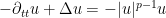

Our main result is that finite time blowup can in fact occur, at least for three-dimensional systems where the number 
Theorem 1 Let
,
, and
. Then there exists a smooth potential
The rather large lower bound of 
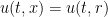
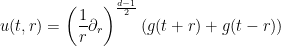
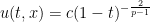
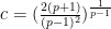
The blowup will in fact be of discrete self-similar type in a backwards light cone, thus
for some fixed 


Because of the discrete self-similarity, the finite time blowup solution will be “locally Type II” in the sense that scale-invariant norms inside the backwards light cone stay bounded as one approaches the singularity. But it will not be “globally Type II” in that scale-invariant norms stay bounded outside the light cone as well; indeed energy will leak from the light cone at every scale. This is consistent with the results of Kenig-Merle and Killip-Visan which preclude “globally Type II” blowup solutions to these equations in many cases.
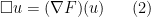
We now sketch the arguments used to prove this theorem. Usually when studying the NLW, we think of the potential 
Now, one cannot write down a completely arbitrary field

we see that

so the defocusing nature of

Furthermore, taking a derivative of (3) we obtain another constraining equation
that does not explicitly involve the potential

where 
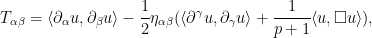
now written in a manner that does not explicitly involve
With this reformulation, this suggests a strategy for locating 


then the question of constructing an (injective) map 

Proposition 2 Let
be a smooth compact Riemannian
-manifold, and let
.
Proof: The Nash embedding theorem (in the form given in this ICM lecture of Gunther) shows that 
![{[-R,R]^{19}}](https://s0.wp.com/latex.php?latex=%7B%5B-R%2CR%5D%5E%7B19%7D%7D&bg=ffffff&fg=000000&s=0&c=20201002)

![{[-R,R]}](https://s0.wp.com/latex.php?latex=%7B%5B-R%2CR%5D%7D&bg=ffffff&fg=000000&s=0&c=20201002)


One can presumably improve upon the bound
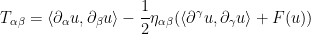
The remaining task is to construct the stress-energy tensor 

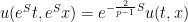
Making the substitution 

(This can be compared with the situation in higher dimensions, in which an undesirable zeroth order term 
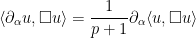
and the potential energy density
then one can verify the equation

which can be viewed as a transport equation for 


I’ve just uploaded to the arXiv the paper “Finite time blowup for an averaged three-dimensional Navier-Stokes equation“, submitted to J. Amer. Math. Soc.. The main purpose of this paper is to formalise the “supercriticality barrier” for the global regularity problem for the Navier-Stokes equation, which roughly speaking asserts that it is not possible to establish global regularity by any “abstract” approach which only uses upper bound function space estimates on the nonlinear part of the equation, combined with the energy identity. This is done by constructing a modification of the Navier-Stokes equations with a nonlinearity that obeys essentially all of the function space estimates that the true Navier-Stokes nonlinearity does, and which also obeys the energy identity, but for which one can construct solutions that blow up in finite time. Results of this type had been previously established by Montgomery-Smith, Gallagher-Paicu, and Li-Sinai for variants of the Navier-Stokes equation without the energy identity, and by Katz-Pavlovic and by Cheskidov for dyadic analogues of the Navier-Stokes equations in five and higher dimensions that obeyed the energy identity (see also the work of Plechac and Sverak and of Hou and Lei that also suggest blowup for other Navier-Stokes type models obeying the energy identity in five and higher dimensions), but to my knowledge this is the first blowup result for a Navier-Stokes type equation in three dimensions that also obeys the energy identity. Intriguingly, the method of proof in fact hints at a possible route to establishing blowup for the true Navier-Stokes equations, which I am now increasingly inclined to believe is the case (albeit for a very small set of initial data).
To state the results more precisely, recall that the Navier-Stokes equations can be written in the form

for a divergence-free velocity field 


purely for the velocity field, where 

An important feature of the bilinear operator

(using the 

This identity (and its consequences) provide essentially the only known a priori bound on solutions to the Navier-Stokes equations from large data and arbitrary times. Unfortunately, as discussed in this previous post, the quantities controlled by the energy identity are supercritical with respect to scaling, which is the fundamental obstacle that has defeated all attempts to solve the global regularity problem for Navier-Stokes without any additional assumptions on the data or solution (e.g. perturbative hypotheses, or a priori control on a critical norm such as the 
Our main result is then (slightly informally stated) as follows
Theorem 1 There exists an averaged version
of the bilinear operator
for some probability space
, some spatial rotation operators
for
, and some Fourier multipliers
of order
, for which one still has the cancellation law
and for which the averaged Navier-Stokes equation
admits solutions that blow up in finite time.


(There are some integrability conditions on the Fourier multipliers
Because spatial rotations and Fourier multipliers of order
It turns out that the particular averaged bilinear operator

where 


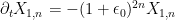
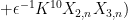
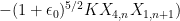
If we consider nonlinearities

where ![{X_n: [0,T] \rightarrow {\bf R}}](https://s0.wp.com/latex.php?latex=%7BX_n%3A+%5B0%2CT%5D+%5Crightarrow+%7B%5Cbf+R%7D%7D&bg=ffffff&fg=000000&s=0&c=20201002)


In principle, if the 


On the other hand, it was shown a few years ago by Barbato, Morandin, and Romito that (3) in fact admits global smooth solutions (at least in the dyadic case 

To get around this, I had to “engineer” an ODE system with similar features to (3) (namely, a quadratic nonlinearity, a monotone total energy, and the indicated exponents of 


where 


The coupling constants here range widely from being very large to very small; in practice, this makes the 


As in the previous heuristic discussion, the time between cascades from one frequency scale to the next decay exponentially, leading to blowup at some finite time 
There is a real (but remote) possibility that this sort of construction can be adapted to the true Navier-Stokes equations. The basic blowup mechanism in the averaged equation is that of a von Neumann machine, or more precisely a construct (built within the laws of the inviscid evolution 

Recent Comments