Polymath8b, IX: Large quadratic programs

21 February, 2014 in math.NA, polymath | Tags: polymath8 | by Terence Tao

This is the ninth thread for the Polymath8b project to obtain new bounds for the quantity

$\displaystyle H_m := \liminf_{n \rightarrow\infty} (p_{n+m} - p_n),$

either for small values of ${m}$ (in particular ${m=1,2}$ ) or asymptotically as ${m \rightarrow \infty}$ . The previous thread may be found here. The currently best known bounds on ${H_m}$ can be found at the wiki page.

The focus is now on bounding ${H_1}$ unconditionally (in particular, without resorting to the Elliott-Halberstam conjecture or its generalisations). We can bound ${H_1 \leq H(k)}$ whenever one can find a symmetric square-integrable function ${F}$ supported on the simplex ${{\cal R}_k := \{ (t_1,\dots,t_k) \in [0,+\infty)^k: t_1+\dots+t_k \leq 1 \}}$ such that

$\displaystyle k \int_{{\cal R}_{k-1}} (\int_0^\infty F(t_1,\dots,t_k)\ dt_k)^2\ dt_1 \dots dt_{k-1} \ \ \ \ \ (1)$

$\displaystyle > 4 \int_{{\cal R}_{k}} F(t_1,\dots,t_k)^2\ dt_1 \dots dt_{k-1} dt_k.$

Our strategy for establishing this has been to restrict ${F}$ to be a linear combination of symmetrised monomials ${[t_1^{a_1} \dots t_k^{a_k}]_{sym}}$ (restricted of course to ${{\cal R}_k}$ ), where the degree ${a_1+\dots+a_k}$ is small; actually, it seems convenient to work with the slightly different basis ${(1-t_1-\dots-t_k)^i [t_1^{a_1} \dots t_k^{a_k}]_{sym}}$ where the ${a_i}$ are restricted to be even. The criterion (1) then becomes a large quadratic program with explicit but complicated rational coefficients. This approach has lowered ${k}$ down to ${54}$ , which led to the bound ${H_1 \leq 270}$ .

Actually, we know that the more general criterion

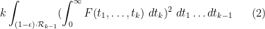
$\displaystyle k \int_{(1-\epsilon) \cdot {\cal R}_{k-1}} (\int_0^\infty F(t_1,\dots,t_k)\ dt_k)^2\ dt_1 \dots dt_{k-1} \ \ \ \ \ (2)$

$\displaystyle > 4 \int F(t_1,\dots,t_k)^2\ dt_1 \dots dt_{k-1} dt_k$

will suffice, whenever ${0 \leq \epsilon < 1}$ and ${F}$ is supported now on ${2 \cdot {\cal R}_k}$ and obeys the vanishing marginal condition ${\int_0^\infty F(t_1,\dots,t_k)\ dt_k = 0}$ whenever ${t_1+\dots+t_k > 1+\epsilon}$ . The latter is in particular obeyed when ${F}$ is supported on ${(1+\epsilon) \cdot {\cal R}_k}$ . A modification of the preceding strategy has lowered ${k}$ slightly to ${53}$ , giving the bound ${H_1 \leq 264}$ which is currently our best record.

However, the quadratic programs here have become extremely large and slow to run, and more efficient algorithms (or possibly more computer power) may be required to advance further.

119 comments

Comments feed for this article

21 February, 2014 at 12:29 pm

Anonymous

“ $sym$ ” –> “ $\mathrm{sym}$ ” (two times)

(Just remove the comment when noted.)

21 February, 2014 at 12:53 pm

Eytan Paldi

Concerning a previous suggestion to work with orthonormal basis, it has the advantage that the matrix $M_1$ (representing the denominator quadratic form) is the unit matrix. So (for such basis) the M-value is simply the largest eigenvalue of the matrix $M_2$ (representing the numerator quadratic form) – which should be simpler to compute (than for the generalized eigenproblem.)

21 February, 2014 at 1:13 pm

James Maynard

I’d just like to try to check in my own mind where we are for the different possible improvements in the unconditional setting. I’ve tried to recall all the main ideas for improvements to the $H_1$ bound, but I’ve probably forgotten one or two.

Use of general symmetric polynomial approximations: Currently implemented, although run-time restrictions mean that we are limited to degree at most about 18 at the moment. Potential to reduce k by 1 or 2 if we can feasibly calculate much larger degrees. Bottleneck is currently calculating the matrices $M_1,M_2$ .

Use of the epsilon trick: Currently implemented. Appears to reduce k by 1 or 2.

Using a piecewise polynomial decomposition: Not implemented. We don’t have a suitable decomposition of our region into a small number of polytopes where we can analytically write down a simple expression for integrating a monomial. For the vanilla region $\mathcal{R}_k$ this would probably only be of minor benefit anyway, whereas when we incorporate other ideas (such as the epsilon trick) we would expect this to make our polynomial approximations converge faster (as the degree increases). Doesn’t change the bound for $M_k$ , but can improve implementation.

Use of support restricted to products of k-1 variables small: Not implemented. This would require a difficult region to integrate over, and we do not know how to do this (as with piecewise polynomial problem). Would probably only reduce k by at most 1.

Functions with larger support but with vanishing marginals: Not implemented. The vanishing marginal condition is very restrictive for relatively low degree approximations unless we can split the support into different polytopes (which we do not know how to do effectively). Numerics from small $k$ suggest that this might not offer much potential improvement when combined with the epsilon trick.

Removing terms $1_{n+h_i,n+h_j}$ prime: Not implemented. Back of the envelope numerics suggest that this is only of small potential benefit for the size of k we are looking at. Since (by parity) we lose a factor of at least 2 in our upper bound, we find that the contribution of these terms (of size roughly $2(\log{k})^2/k^2$ ) is similar to the difference $M_{k-1}-M_k$ . Therefore this appears to only be of potential use if we are stuck at a numerical bound which just fails to decrease k by 1. Would probably only reduce $H_1$ by 2 even if this was the case.

Removing contributions when all the $n+h_i$ are not prime: Not implemented. Any possible benefit expected to be negligible.

Incorporation of Zhang/Polymath 8a technology: Not implemented. Since $2\varpi$ is similar in size to $1/k$ , the smoothness/dense divisibility restrictions to the moduli are rather non-trivial. Unfortunately this means that it appears difficult to obtain a suitably simple integral expression which can be evaluated easily like the monomials. Anything which does avoid the use of e.g. Dickman rho functions appears to throw out too much information to give a non-negligible benefit. There are also (again) issues to do with splitting of the polytope, since we would want to make full use of Bombieri-Vinogradov and only use Zhang/8a to estimate terms from a region outside of this. Would give a noticeable improvement if the restriction to smooth/densely divisible moduli was dropped, but it is slightly unclear to me how much benefit could be expected if this were able to be implemented (it would mainly hurt large divisors, which are the key ones to increase the chances of getting primes).

Would this count as a fair summary? Please correct me if not.

It appears that unless we come up with a effective means of doing a polytope decomposition or of incorporating Zhang/polymath 8a (or some new idea) then the remaining scope for improvement appears to just be enabling a higher degree approximation (by choosing only `good’ monomials, optimising the code, or by doing a larger computation).

21 February, 2014 at 2:21 pm

Eytan Paldi

Concerning the epsilon trick, Terry’s upper bound for
$M_{k, \epsilon}$ implies (at least currently) only that $k > 23$ . If this bound is sufficiently tight (as for the $M_k$ case), there is still some hope for significant improvement.

It should also be remarked that the optimal $F$ should vanish on a certain sub-region of $R$ (disjoint from the supports of the integrands for the numerator functionals $J^{(i)}_{k, \epsilon}(F)$ ) – resulting by a reduced denominator (since its integrand $F^2$ should be integrated over smaller region). Some preliminary analysis shows that this reduction of $F$ support happens only for $\epsilon > 1/(2 k -1)$ and grows with $\epsilon$ .

21 February, 2014 at 6:12 pm

Terence Tao

Yes, this is a good summary of the situation. I had the vague thought that perhaps some other bases than the polynomial basis may possibly provide some speedup (perhaps by making the relevant matrices better conditioned), but the price one pays for this is that the matrix coefficients are unlikely to be rational once we move away from the polynomial setting (e.g. they are likely to involve some logarithms, at the very least) and this will slow things down a lot of we insist on exact arithmetic.

One possible “cheap” way to implement the Polymath8a stuff is to calculate a good near-extremiser for an untruncated simplex, and then naively truncate it to a truncated simplex. But my feeling is that if one does this too crudely, the error terms are too big (because of the $\varpi \sim 1/k$ issue, or more precisely $\delta \sim 1/k$ ), and if one tries to be as sparing as possible with the terms to be cut off then one may be dealing with some tricky 50-dimensional integral for the error terms which does not look appetising at all to compute. In a sense, we’re victims of our own success here; it used to be that k was so large that there were all sorts of good ways to estimate the truncation error, but we’ve manged to get k so low that it is well out of the asymptotic regime (but not yet out of the “curse of dimensionality” regime, alas).

It’s possible that in the future, progress on EH advances to the point where the optimal k drops down to something like k=10 rather than k=50, at which point some of these currently infeasible options become feasible again. (But that would require quite a huge amount of progress on EH, I think.)

21 February, 2014 at 1:37 pm

Terence Tao

Pace, I wonder if you could give a high-level summary of the current methods for bounding $M_k$ and $M_{k,\varepsilon}$ with some estimation of which steps are the most memory and CPU intensive: is it the creation of the matrices $M_1,M_2$ , the inversion of $M_1$ , or the eigenvalue computation for $M_1^{-1} M_2$ that is the biggest cost? Also, I’m curious as to why the eigenvector ends up having rational coefficients rather than algebraic coefficients (or is one just getting an approximate eigenvector instead?).

I do like the idea of using imprecise (but possibly faster) methods to locate a good vector, and then doing a precise (and relatively quick) verification of the required quadratic inequality for that vector – this would also make the claims easier to reconfirm independently. Unfortunately some of the methods suggested so far (e.g. computing determinants of $M_2 - 4 M_1$ ) don’t automatically produce a vector (at least as far as I can tell), although they would still be useful for such tasks as finding the optimal epsilon for a given value of k.

21 February, 2014 at 2:33 pm

Eytan Paldi

It is still possible to compute (sufficiently good) approximation of the eigenvector corresponding to the largest eigenvalue of
$M_2 - 4 M_1$ – which should be useful for confirmation that $M_k > 4$ .

21 February, 2014 at 7:46 pm

Pace Nielsen

Here is a quick high-level summary. (Maybe not so high-level [and maybe not so quick!]. Ignore details as you choose. On the other hand, if you would like more details about any point, just let me know.)

The first step of the computation is finding the entries of symmetric matrices $M_1$ and $M_2$ , corresponding to the $I$ and $J$ -integrals respectively. This is done as described in Maynard’s work. The computation relies on Maynard’s formulas (7.4) and (7.5) from his preprint. These allow one to express the integral over $\mathcal{R}_k$ on a single arbitrary monomial, possibly multiplied by a power of $1-e_1$ , in terms of easily computed rational numbers. Similar formulas over the regions $(1\pm \varepsilon)\mathcal{R}_k$ follow similarly by the obvious substitutions, replacing $1-e_1$ with $1\pm \varepsilon-e_1$ as needed.

Fix some collection of symmetric polynomials $b_n:=b_n(x_1,\ldots, x_k)$ . (Ideally these polynomials are linearly independent.) We then take $F=\sum_{n} c_n b_n$ for indeterminates $c_n$ which correspond to coordinates of the matrices after squaring. In other words, the $(i,j)$ entry of $M_1$ is $\int_{\mathcal{R}_k} b_i b_j\ dx_1\ldots dx_k$ . So we need to find the types of monomials that occur in the product $b_i b_j$ , and how often they occur in order to apply James’ formula. A similar computation is done for the $J$ -integral although this is much slower, as the inner integral involves some expanding of terms. This part of the computation is highly parallelizable and is not memory or CPU intensive; just time intensive. [The computation is affected by the complexity of $\varepsilon$ , as we are doing exact arithmetic. As will be clear a bit later, we could work with real approximations here if necessary. This *might* speed things up, but I doubt it would be by much at present, and we would unfortunately lose our knowledge that the eventual output is a proven lower-bound.]

Currently this step takes a little more than half of the total time. However, some of this time can be saved if one pre-computes a table of the monomials that occur in products $b_i b_j$ and $\left(\int_{0}^{1-\sum_{i=1}^{k-1}} b_i\ dx_k\right)\left(\int_{0}^{1-\sum_{i=1}^{k-1}} b_j\ dx_k\right)$ . This look-up table computation is also highly parallelizable, but at present is memory intensive. If someone wants to work on finding a basis which (1) multiplies well, (2) integrates well with respect to the inner $J$ -integral, and (3) from which it is easy to find which monomials occur, that would be very useful. In particular, finding an algorithm to count the number and types of monomials in $e_1^{a_1}e_2^{a_2}\cdots e_k^{a_k}$ which is not memory intensive (and which is somewhat quick) would be very helpful. [I imagine this is not a hard problem. I just haven’t thought about it yet.]

At present, the second step in the computation is to find the *exact* inverse of $M_1$ . This is the most memory intensive part of the program, and simply won’t run in Mathematica without more than 64GB of RAM, when the degree gets to be about 20-22. I’m currently playing with the other option that has been discussed recently, of instead just solving the generalized eigenvalue problem. I don’t know yet if this is less memory intensive (as implemented in Mathematica), but I believe it probably is.

The third step is to compute $M_3= M_1^{-1}M_2$ exactly. This is relatively quick and easy.

Fourth, we compute a real approximation $M_3'$ to $M_3$ . This step is also very quick. In the past we’ve been using 150 digit approximations in every entry, but I’m currently thinking this may have been extreme overkill (and may slow down subsequent steps). We may be able to get by with many fewer digits (but not too many fewer, I’m still experimenting with this).

Fifth, we find an eigenvector $x'$ of $M_3'$ , corresponding to the largest eigenvalue. This step is not too long, nor too memory intensive; but I haven’t been able to explore this step in the past because the computation of $M_1^{-1}$ was usually the hang-up. We will likely replace this step with finding the generalized eigenvector. I expect the new computation to take about the same time as the old, but I don’t have a lot of data yet.

Sixth, we find a rational approximation $x$ of the vector $x'$ . This is again very quick and easy.

Finally, we compute $(x^{T}M_2 x)/(x^{T}M_1 x)$ using exact arithmetic. This is very quick, and the output is a proven lower bound on $M_{k,\varepsilon}$ .

If the generalized eigenvector functionality in Mathematica turns out to be less RAM intensive, then the new difficulty will be in building the look-up table for large degrees.

21 February, 2014 at 8:39 pm

Eytan Paldi

It should be remarked that since $M_3$ is not symmetric, some of the eigenvalues (and corresponding eigenvectors) of $M'_3$ may be complex (in particular, for clusters of eigenvalues). A related problem is that the algorithm for the eigenproblem of nonsymmetric $M_3$ is in general slower (with less numerical stability) than the corresponding algorithm for the generalized eigenproblem with the symmetric positive definite matrices $M_1, M_2$ .

22 February, 2014 at 6:52 am

andre

The numerical analysis mathematican’s standard questions are
1. Do you really need the matrices explicitly in memory?
2. Wouln’t it suffice to only use matrix-vector-products?
3. If your matrices are symmetric what could you say about their
L.D.L^T decomposition?
4. Is it possible to factor the L matrices again?

So perhaps on needs to check if there are somehow better polynomials
for easier decomposition of the $M_1$ and $M_2$ matrices.

22 February, 2014 at 7:33 am

Pace Nielsen

I woke up this morning, and realized there is the potential to get a huge speed up when doing multiple runs of the computation of the $J$ -integral by creating a second look-up table.

The first look-up table, for the $I$ -integral, yields the the number and types of monomials occurring in a product $b_i b_j$ . For the $J$ -integral, we first explicitly compute $\left(\int_{0}^{1-\sum_{t=1}^{k-1}x_t} b_i\ dx_k\right)\left(\int_{0}^{1-\sum_{t=1}^{k-1}x_t} b_j\ dx_k \right)$ , re-express this as a linear combination of products $b_i' b_j'$ , and then use the first look-up table. Ultimately, it would make more sense to just have a separate look-up table for these more complicated products (possibly still using the first look-up table to construct the second one).

22 February, 2014 at 8:08 am

Eytan Paldi

Pace, does “explicitly compute” means using symbolic computation?
(I’m asking that because symbolic computation can take much more time than numerical one).
Perhaps symbolic computation may be made only once (to prepare an additional table for the coefficients of the above linear combination of products – since these coefficients are dependent only on the indices $i ,j$ of the above products.)

22 February, 2014 at 10:12 am

Pace Nielsen

Right! The idea is to do the (symbolic) computation once to form the look-up table of coefficients.

22 February, 2014 at 1:46 am

Aubrey de Grey

Way back in https://terrytao.wordpress.com/2013/11/19/polymath8b-bounded-intervals-with-many-primes-after-maynard/#comment-251896 James gave approximate values for the entirely unenhanced M_k for k=10, 20 etc. I just realised that those entries can easily be checked using the code developed by James and Pace for use on k in the 50’s, and moreover that this can give at least a provisional guide to the dependence of M on d for values of k across the whole range still of interest. Accordingly, and after checking that the code duly gives the same M_k for k=3 and 4 that were obtained using other methods, I did a few runs and obtained the following improved values:

k=5: d=5, M=2.00679…
k=10: d=8, M=2.54478…; d=10, M=2.54534…
k=20: d=8, M=3.11055…; d=10, M=3.12136…; d=12, M=3.12543…
k=30: d=8, M=3.41946…; d=10, M=3.45095…; d=12, M=3.46744…
k=40: d=8, M=3.60972…; d=10, M=3.66230…; d=12, M=3.69443…
k=50: d=8, M=3.73521…; d=10, M=3.80574…; d=12, M=3.85268…

I’m presuming these are reliable; at least they do not contravene the upper bounds previously determined. But it’s interesting that they are so much closer to those bounds than the estimates we had before, and also that there is non-trivial dependence on d throughout, albeit diminishing as d approaches k.

I also did a little survey for k = 10 through 50 with Pace’s latest code that incorporates epsilon. Here are the optimal values that come out using d=10, with values for epsilon drawn only from reciprocals of integers:

k=10, eps=1/9, M=2.68235…
k=20, eps=1/15, M=3.21470…
k=30, eps=1/23, M=3.51943…
k=40, eps=1/34, M=3.71480…
k=50, eps=1/46, M=3.84772…

I think it would be possible to use small-d calculations of this kind to obtain a more accurate idea of how the optimal epsilon varies with d for a given k, leading to a better guess for what epsilon to explore in the highly CPU-intensive calculations currently in progress for k=52. I’ll probably have a go at that soon.

22 February, 2014 at 7:23 am

Pace Nielsen

If you are just using my code as-is, then these values are not reliable. You would need to add the restriction that signatures are limited to lengths at most size $k$ . (Now that I think about it, this should be an easy change. In the TermIntegral function, just return 0 if the length of T is larger than k. [You might also want to restrict the symmetric function generator as well.])

That said, thank you for this work! I hope you continue to find patterns, as these will be helpful.

22 February, 2014 at 9:21 am

Aubrey de Grey

Pace: I remembered your earlier comment about this, but I’m confused – I’m not (yet) exploring values of d exceeding k, so surely this issue doesn’t yet arise? (Indeed, since you exclude signatures with any element equal to 1, surely it wouldn’t arise until d exceeds 2k?) Please clarify. At any rate, I’ve made the change you suggest and for a couple of sample parameters I’m getting the same values I posted above.

22 February, 2014 at 10:09 am

Pace Nielsen

When computing the integrals you are squaring quantities. So for instance, when $k=10$ and $d=10$ , you will be squaring $m=m(2,2,2,2,2)$ , one term of which is $m(2,2,2,2,2,2,2,2,2,2)$ . This would (barely) have been okay, except that when computing the $J$ -integral (after the initial integration, one summand of which leaves $m$ alone) we now only have $k=9$ variables. (So, this probably does not have a large effect, but it does exist.)

22 February, 2014 at 10:32 am

Pace Nielsen

Looking more closely, the d=10, k=10 case should have been the only one where this problem arises.

22 February, 2014 at 11:11 am

Aubrey de Grey

Ah, I get it – many thanks. Yes, I’d just reached the same conclusion (we’re safe until d=k, and also for d=k when k is odd). Actually there seems to be some subtler reason why the specific case d=k, k even is also OK, because I’m not seeing a change in values even at 50-digit precision from excluding that signature. (By the way, for simplicity of audit trail I’m now only using your latest code, specifying epsilon as zero as desired.)

22 February, 2014 at 3:31 am

turcas

Reblogged this on George Turcas.

22 February, 2014 at 10:40 am

Pace Nielsen

One more data point. I ran the $d=22, \varepsilon=1/30, k=51$ computation (using only signatures with even entries) and got $M_{51,1/30}\geq 4.011910$ . This means we are down to $H\leq 252$ , and it looks probable that we can reduce $k$ once more with minimal effort.

It took 1 day 5 hours to form the matrices (not counting the time to make the look-up table). It took 2 hours to find the inverse matrix. Finally, it took a little less than 4 hours to find the eigenvector.

I also ran the generalized eigenvector computation, got the same answer, only used 50 digits real approximations, and the computation took 2.5 hours (as opposed to the 6 hours above).

I wasn’t near the computer during these computations, so have no idea about the RAM needs of each step (except that the matrix formation step didn’t require much RAM at all).

22 February, 2014 at 10:57 am

Terence Tao

Nice! Great to see that the improved matrix computation performance is translating into tangible gains in the degree, and thence in the value of k and H. (Amusingly, this already makes obsolete the value of H given in the recent survey of Ben Green at http://arxiv.org/abs/1402.4849 .) The fact that the two different matrix computations arrive at the same answer is also reassuring :)

22 February, 2014 at 12:05 pm

Eytan Paldi

Is it possible that the optimal $\epsilon$ (which by now is $1.7/k$ ) could be much larger than $1/k$ (for sufficiently large degree)?

Perhaps the dependence of optimal $\epsilon$ on the degree may be explained by the fact that the optimal $F$ vanishes on a certain simplex (whose size is growing with $\epsilon$ ) inside the whole simplex $R$ – so for polynomial approximation with larger degree it is easier to approximate zero (the value of optimal $F$ ) on this inner simplex for larger values of $\epsilon$ .

This indicates the possibility that by taking this inner simplex into account by taking the integral in the denominator over the (true) reduced support of $F$ , it may be possible to get much larger values of optimal $\epsilon$ (without using very large degrees) with larger M-values (for the same $k$ ).

22 February, 2014 at 1:43 pm

Aubrey de Grey

I’m currently doing some more precise computations of the optimal epsilon (using a simple binary chop) for small k and for d ranging up to k, and the trend seems to be that the optimal epsilon peaks when d is k-1 or k-2, and for d=k (which, unsurprisingly, always gives the best M) the optimal epsilon exceeds 1/k by a number that grows slowly with k, but the absolute value of the optimal epsilon for d=k still falls with increasing k. (Incidentally, I’m not exploring d exceeding k, because the code is throwing me singular-matrix errors then, but the growth of M (for optimal epsilon) with d decelerates really sharply as d approaches k so I don’t think this is an urgent issue.) I think when d=k=40 or 50 we will be looking at an optimal epsilon between 0.05 and 0.1, but I’ll be more confident once I’ve gathered more data points.

22 February, 2014 at 2:48 pm

Eytan Paldi

The (exact) matrix $M_1$ representing the denominator quadratic form should be positive definite for each degree $d$ (since we are working with linearly independent basis functions) – therefore its apparent singularity (for $d > k$ ) shows that there is some bug in the implementation of the algorithm!

More interesting than the behavior of optimal $\epsilon$ is the behavior of $k \epsilon$ (for optimal epsilon) – is it growing with $d$ (for each fixed $k$ )? could you please give some data about it (for several pairs $(k, d)$ ) to illustrate its behavior?

22 February, 2014 at 3:03 pm

Aubrey de Grey

Pace just confirmed to me that he does not expect his code to work for d greater than k, so there’s no concern there. As to your question, can you clarify? – clearly for a fixed k, ke grows with d iff e does, so I must not be understanding your question.

I’ll have some reasonably comprehensive trend summaries later today.

22 February, 2014 at 3:28 pm

Eytan Paldi

Concerning the behavior of $k \epsilon$ with respect to $d$ you are right (of course), but it is also interesting to see its behavior wrt $k$ (for sufficiently large d).
I have some indication (from a preliminary analysis) that optimal $\epsilon$ is decaying more slowly than $1/k$ . (i.e. that $k \epsilon$ for sufficiently large $d$ should grow unboundedly with $k$ ).

22 February, 2014 at 3:45 pm

Aubrey de Grey

Got it. So far I only have data for small d, but I can say that for d=5, ke rises with k at first but peaks at 1.097 when k=11 and is down to 0.67 by k=50. The peak for d=4 is also at k=11, but for d=3 it’s falling with rising k all the way from k=3, so I’ll have to look at slightly higher d to know what’s really going on here.

22 February, 2014 at 3:58 pm

Eytan Paldi

In other words, the idea is to estimate the “large d limit” of $k \epsilon$ for each fixed $k$ , and see its behavior as a function of $k$ .

22 February, 2014 at 4:08 pm

Aubrey de Grey

Well, now you’re confusing me again – that would be the same as the behaviour of the “large d limit” of epsilon as a function of k, which is as I noted above – it’s slightly over 1/k.

22 February, 2014 at 4:38 pm

Eytan Paldi

The meaning of the “large d limit” of $k \epsilon$ (for each fixed k) is simply to estimate the limit of $k\epsilon$ as $d$ tends to infinity. (e.g. for the current k=51 and $\epsilon = 1/30$ it seems that this limit should be larger than 51/30 = 1.7).
As stated above, $\epsilon > 1/k$ , so we know that this limit is larger than 1 and grows with k, but how fast it grows, as a function of k? (is it unbounded for large k, as I think, or not?)

22 February, 2014 at 4:43 pm

Pace Nielsen

Regarding the $d$ bigger than $k$ case: The old code should not work here, because the set of symmetric polynomials of the form $(1-e_1)^a m(\alpha)$ (with the signature $\alpha$ having entries bigger than 1) does not remain linearly independent when the degree of the signatures ranges over all possibilities up to and exceeding $k$ . (Try the case when $k=1$ for instance.) However, as far as I know, this should not cause a problem in the generalized eigenvector set-up (other than to slightly slow things down).

22 February, 2014 at 4:46 pm

Aubrey de Grey

Ah, OK. Well, as noted, I can’t test values of d exceeding k using Pace’s current code. I would expect that the best epsilon continues to rise with d beyond k for any fixed k, but I’m not sure that that’s worth exploring, because M seems to be very nearly maximal (i.e. it is growing with d much more slowly than before) before d reaches k.

22 February, 2014 at 5:05 pm

Eytan Paldi

What is really interesting is the behavior of the “large d limit” of $k \epsilon$ . Is it bounded as a function of k (as previously assumed), or is it unbounded (as seems to me now)?
If it is unbounded, the optimal $\epsilon$ can be much larger (with sufficiently large d) – which may indicate a significant improvement in k.
(Note that the current upper bound on $M_{k, \epsilon}$ implies only that $k > 23$ ).

22 February, 2014 at 1:59 pm

Aubrey de Grey

Just to fill in the gap in the world-records column of current interest: for k=5, d=5 I get M=2.20264… (with an optimal epsilon of 0.2048).

[Added, thanks – T.]

22 February, 2014 at 4:12 pm

Aubrey de Grey

Here’s a question I just asked Pace but he thought others (especially Eytan, I suspect) might have a better idea. I checked k=d=4 using Pace’s code, and the best M I get is 2.062926693 (with epsilon = 0.22956). This is greater than the value of 2.01869 that Pace obtained with epsilon=0.18 (in https://terrytao.wordpress.com/2013/12/20/polymath8b-iv-enlarging-the-sieve-support-more-efficient-numerics-and-explicit-asymptotics/#comment-262158), so I tried that value of epsilon and I still got a bigger value than Pace’s, 2.054687. So, remembering the issue of signatures of length exceeding k, I stepped back to d=3 – but I get 2.045786, still well above Pace’s value. Should I be worried about this? I don’t properly understand the maths behind Eytan’s idea described in https://terrytao.wordpress.com/2013/12/20/polymath8b-iv-enlarging-the-sieve-support-more-efficient-numerics-and-explicit-asymptotics/#comment-261838 (which was the basis of Pace’s computation), so I thought I should check.

22 February, 2014 at 4:37 pm

Terence Tao

If you can post (or put on dropbox) the polynomials used, say for d=3, together with the J and I values, I could verify them with Maple.

22 February, 2014 at 4:40 pm

Aubrey de Grey

Many thanks! However, here I’m using the code that Pace developed for large k, from which I don’t know how to extract the explicit polynomials. If Pace can offer guidance on how to do that, I’ll do as you suggest.

22 February, 2014 at 5:31 pm

Pace Nielsen

I double checked it and my program seems to work out. Take $k=4, \varepsilon=18/100$ . Let $c_1,\ldots, c_7$ be the entries of

{35958260/235553951, -(50078641/92388318), 79192071/282465067, -(
48604192/195227029), -(78520320/199602007), -(81680335/
131295067), 8512013/371894111}

Take $F=c_1*1 + c_2*p_2 + c_3 p_3 + c_4*(1+\varepsilon-e_1) + c_5*(1+\varepsilon-e_1)p_2+c_6*(1+\varepsilon-e_1)^2+ c_7(1+\varepsilon-e_1)^3$ where $e_1=x_1+x_2+x_3+x_4$ , $p_2=x_1^2+x_2^2+x_3^2+x_4^2$ and $p_3=x_1^3+x_2^3+x_3^3+x_4^3$ .

You should get $M_{4,18/100}\geq 2.04579$ .

22 February, 2014 at 8:06 pm

Terence Tao

I actually get $M_{4,18/100} \geq 2.045655896$ from this, but I’ll call it close enough (presumably it is coming from rounding the eigenvector?).

eps := 18/100;


c1 := 35958260/235553951;

c2 := -(50078641/92388318);

c3 := 79192071/282465067;

c4 := -(48604192/195227029);

c5 := -(78520320/199602007);

c6 := -(81680335/131295067);

c7 := 8512013/371894111;
e1 := x1+x2+x3+x4;

p2 := x1^2+x2^2+x3^2+x4^2;

p3 := x1^3+x2^3+x3^3+x4^3;

F := c1*1 + c2*p2 + c3 *p3 + c4*(1+eps-e1) + c5*(1+eps-e1)*p2+c6*(1+eps-e1)^2+ c7(1+eps-e1)^3;
Iint := int(int(int(int(F*F, x4=0..1+eps-x1-x2-x3),x3=0..1+eps-x1-x2),x2=0..1+eps-x1),x1=0..1+eps);
marginal := int(F, x4=0..1+eps-x1-x2-x3);
Jint := 4 * int(int(int( marginal*marginal, x3=0..1-eps-x1-x2), x2=0..1-eps-x1), x1=0..1-eps);

evalf(Jint/Iint);

22 February, 2014 at 9:19 pm

Pace Nielsen

That discrepancy is strange! It isn’t round-off on my end. The value I’m getting for Jint/Iint (using those rational coefficients) is exactly

2875735523016629068741175964840742575048112964757776538183474000859721435716670538831465909183618392849627156512838669025828999932027/
1405687353551049804337736122604236419384565626408790839655020559027003306701017406210501472288913119227666603789342318453993312108750

So $M_{4,18/100}\geq 2.045786010489\ldots$ . Maybe round-off error on your end?

22 February, 2014 at 10:13 pm

Terence Tao

I am getting

Jint/Iint =

112805940582930117839342308454515665732548154445069213111398986990206498514376044710654769998982151256045268574930189154070867853942748204311984028009988367010311873424
/
55144142657853654365564445664600642139014017 646291100083550438379226357318392264559974985439172491855197950450119863075917734899756314238903142624644107058773523923075

with

Jint= 7050371286433132364958894278407229108284259652816825819462436686887906157148502794415923124936384453502829285933136822129429240871421762769499001750624272938144492089
/
1503397131218453159163272735128833401375525832080327795183919892914673536996939361897130816655717647821109961157503227305815102605266463600374304201477050781250000000000
= 0.004689626673

and

Iint=353658121903823340487827132689438141023017589522469777672281150419922124857413914125220365170258084689420878307647029507248580405684234336399824432541972478906679
/
154268745226841433680374306634993326419807043856246559069698369643320677197056468111939028805460845695929192743434674599281973010641420026333101601562500000000000000
= 0.002292480706

so there is some weird discrepancy here that we should probably track down. (My maple code is just the one posted above, so if you have maple, you may be able to do a side-by-side comparison with your Mathematica code.)

23 February, 2014 at 1:04 am

Anonymous

I’m getting the same as Pace Nielsen; see http://speedy.sh/revYz/output.jpg.

23 February, 2014 at 5:43 am

Pace Nielsen

I ran your code in Maple and got the same answer as you did. Then I added the symbol * in the definition of F after the c7, reran the code, and got my answer. It is amazing how picky these computing platforms can be!

23 February, 2014 at 8:30 am

Terence Tao

Ah, so that was it! (Actually, it would have been better if Maple was _more_ picky, and complained on the lack of *, rather than silently deciding to treat constants as functions (which I suppose is a useful convention elsewhere…).) Anyway, good catch – I had scanned over the code several times and didn’t pick it up.

22 February, 2014 at 5:33 pm

Eytan Paldi

Aubrey: that comment of mine was for the exact computation of $M_{k, \epsilon}^{1D}$ – a (1D) modification for $M_{k, \epsilon}$ .

22 February, 2014 at 5:41 pm

Aubrey de Grey

Ah, excellent – thanks – I didn’t realise it was for d=1. I get 2.0055 as the best M for k=4 and d=1 (the epsilon being 0.16841). Does the fact that your value of 2.01869 is slightly bigger imply that there is still some unexplored space here? – for example, scope to increase M using partitioning, or non-polynomials? (0.003 isn’t much, but I guess there might be a greater disparity for larger k and/or d.)

22 February, 2014 at 6:00 pm

Eytan Paldi

This M-value modification is for optimizing $F(t_1,...,t_k)$ of the particular (1D) type: $F = f(\sum_i t_i)$ , where $f$ is a function of one variable. Therefore this M-value is smaller than the usual (with more general F) $M_{k, \epsilon}$ .

The optimal $f$ is not a polynomial (so the degree d is meaningless here!)

22 February, 2014 at 4:57 pm

Terence Tao

Some comments on trying to implement the Polymath8a stuff. For simplicity I’ll only work with the $MPZ[\varpi,\delta]$ estimates and not the more complicated $MPZ^{(i)}[\varpi,\delta]$ estimates. I’ll also avoid any use of the Dickman function, which in principle can be used to claw back a lot of the losses from the truncation to smooth moduli, but looks very complicated to analyse and implement.

Let A denote the region of integration for the J functional, and B the support of the F marginal $\int F\ dt_k$ . Right now we are taking $A = (1-\varepsilon) \cdot {\cal R}_{k-1}$ and $B = (1+\varepsilon) \cdot {\cal R}_{k-1}$ . The key relation between these two sets is that whenever $(a_1,\dots,a_{k-1}) \in A$ and $(b_1,\dots,b_{k-1}) \in B$ , we have

$a_1+\dots+a_{k-1}+b_1+\dots+b_{k-1} \leq 2$ (*)

which roughly speaking means that we can use the Bombieri-Vinogradov theorem to control interactions between A and B.

If we use $MPZ[\varpi,\delta]$ instead of Bombieri-Vinogradov for some fixed choice of $\varpi,\delta$ , we get to replace this condition (*) with the conjunction of

$a_1+\dots+a_{k-1}+b_1+\dots+b_{k-1} \leq 2 (1+4\varpi)$ (**)
and

$a_1,\dots,a_{k-1},b_1,\dots,b_{k-1} \leq 4\delta.$ (***)

The condition (**) is more generous than (*), but the price one pays for this is the new restriction (***).

By the way, it would be OK if for some choices of $(a_1,\dots,a_{k-1}) \in A$ and $(b_1,\dots,b_{k-1}) \in B$ , we had (*), whilst for other choices one had (**) and (***), and one could also have $\varpi,\delta$ vary with the a and b’s. But for simplicity I’ll stick with a single choice of $\varpi,\delta$ and just use (**) and (***) for that choice. Then one natural choice for the polytopes A,B would be

$A = \{ (a_1,\dots,a_{k-1}: a_1+\dots+a_{k-1} \leq (1-\varepsilon)(1+4\varpi);$
$a_1,\dots,a_{k-1} \leq 4\delta \}$

$B = \{ (b_1,\dots, b_{k-1}): b_1+\dots+b_{k-1} \leq (1+\varepsilon) (1+4\varpi);$
$b_1,\dots,b_{k-1} \leq 4\delta \}$

so one could try to maximise the ratio J/I for functions F supported on $\{ (t_1,\dots,t_k): t_1+\dots+t_k \leq (1+\varepsilon)(1+4\varpi); t_1,\dots,t_k \leq 4\delta\}$ , with the J integration being on A.

Our most optimistic numerology for $\varpi,\delta$ currently is roughly $83 \varpi + 25 \delta < 1$ , so if we split the difference we could take for instance $\varpi \approx 1/166, \delta \approx 1/50$ . The enlarging of the simplex by $1+4\varpi \approx 1.02$ is in principle equivalent to lowering the threshold for $M_k$ from 4 to about 3.92, which would in principle reduce k by about 5. But we have to truncate all the coefficients $t_i$ to $4\delta \approx 4/k$ , which looks like a pretty serious truncation. If $t_1,\dots,t_k$ are chosen uniformly on the simplex, then each $t_i$ behaves roughly like an exponential random variable of mean $1/k$ , so that it hits $4/k$ pretty often. I’m not exactly sure how things change when one weights by F^2, but from the large k analysis it looks like each of the $t_i$ behave like Cauchy random variables of mean about 1/k, so asking for all k of these variables to stay below $4/k$ looks like quite a big ask. So this suggests that the “naive” strategy of taking an optimiser for the untruncated problem and simply lopping off the regions where $t_1,\dots,t_k \geq 4\delta$ may give poor results. (But this doesn’t preclude a direct optimisation of the truncation problem giving better results than what we currently have, although we are still faced with the difficult problem of computing the relevant integrals such as $\int b_j b_k$ properly.)

22 February, 2014 at 9:41 pm

James Maynard

Note that if we restrict all variables to be less than $c/k$ and drop all other restrictions, the optimal function is just a constant (by Cauchy-Schwarz), which then gives a ratio of $c$ . So the $c=4$ case from above will certainly be too restrictive.

22 February, 2014 at 10:22 pm

Terence Tao

Good point! We have the room to double $\delta$ , but this gives up all the gain in $\varpi$ . So it may well be that k is now too small for the Polymath8a estimates to be of much use.

In principle we can be much less drastic than forcing all of the $t_k$ to be bounded by $4\delta$ ; it should be enough that most of them are bounded by this, as long as the exceptional ones are not too huge (here we would need the more refined $MPZ^{(i)}$ estimates that only require dense divisibility on the moduli). Then there is also the Dickman function card to play, since a significant fraction of those numbers above $x^\delta$ would still be $x^\delta$ -smooth. This all looks rather complicated though (and may not play well with the epsilon trick, which is currently giving almost all of our recent improvements).

23 February, 2014 at 2:42 pm

Aubrey de Grey

I’ve been exploring variations on Pace’s initially-accidental restriction of monomial signatures to those in which all elements are even, and I can report substantial progress (although the pattern of which values give the best trade-off between execution time and M remains thoroughly mysterious).

I’ve been using k=20 as a benchmark. The bottom line is that it’s essential to include 2 in signatures in order to keep M competitive, but thereafter we can be quite sparse with not much loss in M. A fairly thorough survey using d=6, 10, 12 and 14 reveals that, relative to using all even numbers, particularly good performance arises from restricting signature entries to just the values 2, 6 and 10 – it loses only about 0.02 in M (which equates to about one increment of k at present), and it improves execution time by a factor of 4 for d=10, 7 for d=12 and 13 for d=14. I don’t have a feel for what are the ideal subsequent numbers to allow in signatures (presumably some will be needed to maintain an acceptable shortfall in M as k rises), but 4n+2 should be pretty good.

I don’t know whether these speed gains will still be so big after the new code enhancements (especially the second lookup table), and I also don’t know what the RAM implications are, but I’d hope this will still help quite a bit in progressing us to the goal of computing M for d=k for k in the 40-50 range. (Simplistically it would seem to get us to computability of d=40 on its own, but let’s see!)

23 February, 2014 at 4:05 pm

anon

“us”?

23 February, 2014 at 5:57 pm

Aubrey de Grey

Update: it seems that adding back 8 as an admissible member of signatures makes more and more difference to M as k rises, and with only modest impact on execution time. It may be that for k in the region of current interest most of the benefit in execution time from these restrictions on signatures (over and above just restricting to even numbers) arises just from deleting 4 from the list of allowed values, i.e. from using 2, 6, 8, 10, 12 etc. Deleting both 4 and 6 costs too much in M for d up to 16, but is probably the next thing to look at for d in the 20s (which is beyond my puny MacBook’s ability to explore using the currently-available code).

24 February, 2014 at 2:22 am

Johan Commelin

Is there a central repository with up to date code/notebooks? On the wiki there are some notes by Pace Nielsen, but all the other code is rather outdated. I can imagine that a github repository, or maybe just a dropbox directory could really help. Currently there are some snippets of code in the comments, but I have a hard time finding the most current versions…

24 February, 2014 at 6:50 am

Aubrey de Grey

The repository being used at present is https://www.dropbox.com/home/Polymath8/Polymath8b . The code from Pace that was deposited there on Feb 19th doesn’t have the latest ideas (precomputing a second lookup table for the J matrix, restricting the values allowed in signatures) but otherwise I think it has everything that has been discussed here concerning the unconditional (i.e. theta=1/2) setting).

24 February, 2014 at 6:55 am

Johan Commelin

Is it possible that the link you provided is not public? Even with a dropbox account I cannot access it.

24 February, 2014 at 6:58 am

Aubrey de Grey

Ah – I’m not sure, since I only accessed it after receiving an “invitation” email from Terry. I’m sure Terry will advise.

24 February, 2014 at 8:38 am

Anonymous

I’m rather sure that Terry needs to invite Johan Commelin before he can get access to the folder.

24 February, 2014 at 8:57 am

Eckhard

https://www.dropbox.com/sh/j2r8yia6lkzk2gv/raL055WXr5/Polymath8b is the correct dropbox link, I believe.

25 February, 2014 at 9:40 am

Aubrey de Grey

James – concerning your summary in https://terrytao.wordpress.com/2014/02/21/polymath8b-ix-large-quadratic-programs/#comment-272402 of the situation regarding functions with larger support than R_k,epsilon but with vanishing marginals, I am wondering about two ideas raised in posts from December:

1) In https://terrytao.wordpress.com/2013/12/08/polymath8b-iii-numerical-optimisation-of-the-variational-problem-and-a-search-for-new-sieves/#comment-256158 Pace proposed (based on something he credited to you) a relatively simple way to dissect R’_k that seems not to involve any marginals (but does it work for R’_k,epsilon?);

2) In https://terrytao.wordpress.com/2013/12/20/polymath8b-iv-enlarging-the-sieve-support-more-efficient-numerics-and-explicit-asymptotics/#comment-258264 Terry proposed (and Pace refined in https://terrytao.wordpress.com/2013/12/20/polymath8b-iv-enlarging-the-sieve-support-more-efficient-numerics-and-explicit-asymptotics/#comment-258471) a method for satisfying marginals automatically on 2R_k.

Do either of these lines of thought lead to a more optimistic prognosis for going beyond R_k,epsilon, at least for large k and d? (I ask especially because the past day’s exploration has sharply reducied my earlier optimism concerning improvements to the trick of only allowing even numbers in monomials.)

26 February, 2014 at 3:34 pm

interested non-expert

Hello!
In this weeks issue of Nature journal, there is a small text about scientific crowd-sourcing. Among others, about this polymath project
http://www.nature.com/news/parallel-lines-1.14759?WT.ec_id=NATURE-20140227

28 February, 2014 at 4:51 pm

Anonymous visitor

As a visitor who knows very little about this, I wonder if there is some form to the functions F that satisfy condition 1 particularly well. I mean, can one construct such a function to be ideal? And I wonder about the constant 4, what is the maximum such constant for each k (assuming equality is included)?

1 March, 2014 at 10:25 am

Terence Tao

This is a great question. For large k (setting epsilon to zero for simplicity), it appears that functions F that are roughly of the form $F(t_1,\dots,t_k) := \prod_{i=1}^k \frac{1}{1+At_i}$ for a well-chosen parameter A works quite well, though it is not quite the optimal function. For k=2, which is the only case in which we have found the exact optimiser, the optimal function F (when epsilon is zero) is the rather strange function

$F(t_1,t_2) = \frac{1}{M_2-1+t_1} + \frac{1}{M_2-1+t_2} + \frac{1}{2M_2-1} \log \frac{M_2-t_1}{M_2-1+t_1} \frac{M_2-t_2}{M_2-1+t_2},$

where $M_2 = 1/(1-W(1/e)) = 1.38593...$ . This unfortunately does not give many clues as to what the general structure of the optimiser is like.

We’ve used $M_k$ to denote the optimal value of the constant in place of 4 (at least in the simpler case $\varepsilon=0$ ). The best lower and upper numerical bounds on this quantity that we have can be found at http://michaelnielsen.org/polymath1/index.php?title=Selberg_sieve_variational_problem#World_records . Asymptotically we know that $M_k= \log k + O(1)$ , so we can exceed 4 for k large enough; the challenge is to exceed 4 for explicit values of k such as 50.

28 February, 2014 at 5:27 pm

Warren D Smith

Just on grounds of mathematical naturalness alone, it seems to me that
you might want to consider putting in nonpolynomial factors of
exp(A*(x1+x2+…+xk))
into the ansatz definition for F, for various constants A.

1 March, 2014 at 10:32 am

Terence Tao

I played around with this some time ago. When working with functions $F(t_1,\dots,t_k)$ that is homogeneous of degree d, thus $F(\lambda t_1,\dots,\lambda t_k) = \lambda^d F(t_1,\dots,t_k)$ for all $\lambda>0$ , then there is a clean relationship between integration on the solid simplex, the boundary, and against exponential weights: we have

$\int_{t_1,\dots,t_k \geq 0} e^{-a(t_1+\dots+t_k)} F(t_1,\dots,t_k)\ dt_1 \dots dt_k$
$= a^{-d-k} \Gamma(d+k) \int_{t_1+\dots+t_k=1} F(t_1,\dots,t_k)\ dt_1 \dots dt_{k-1}$
$= a^{-d-k} \Gamma(d+k+1) \int_{t_1+\dots+t_k \leq 1} F(t_1,\dots,t_k)\ dt_1 \dots dt_k$

which was useful for us in integrating monomial functions on the simplex. Unfortunately, when F is not homogeneous, then the relationship is much messier and we have not been able to exploit it. If one adds in weights such as $\exp(A(t_1+\dots+t_k))$ , then one begins to see the incomplete Gamma function appear in the formulae, and this does not look very appealing (especially since our current optimisation methods rely on writing all the coefficients as exact rationals).

1 March, 2014 at 9:01 pm

Anonymous

@TT: What’s going on in the last line of your comment? :)

[Deleted, thanks – T.]

1 March, 2014 at 5:17 pm

arch1

It seems odd that a post such as this received so many downvotes, when the blog host has advised that downvoting be used sparingly. (Posted in the possibly-vain hope that this will be taken as food for thought rather than as fodder for debate:-)

[This was possibly related to a further comment on this post which has since been deleted. -T]

28 February, 2014 at 5:43 pm

Warren D Smith

Or, if you could reformulate the problem somehow to change the region of integration from being x1>0, x2>0, …, xk>0, x1+x2+…+xk< 1; x1> 0, x2>0, …, xk>0, but now with the weighting function exp(-x1-x2-…-xk), then that would be more natural. I’m saying this out of total ignorance of where this comes from, but just because it is a common experience that you get nicer results in problems of this sort if you can do this.

Another more-elegant region of integration (if it can be done) is
the REGULAR simplex x1>0, x2>0, …, xk>0
with x1+x2+…+xk=1 (this is 1-less dimensional).

3 March, 2014 at 7:54 am

Terence Tao

A podcast discussing bounded gaps between primes and Polymath8: http://podacademy.org/podcasts/maths-isnt-standing-still/

4 March, 2014 at 3:00 am

luoyu4304

Professor Tao, I am an amateur in number theory. I’ve been paying attention to this project for a couple of month. When I heard the big news of Zhang’s breakthrough in the twin prime conjecture, I began to search for more information about Zhang and the conjecture. At first, I tried to read Zhang’s paper, but soon I found it too difficult for me. Then I learned elementary number theory and a little analysis number theory by myself, and read the paper again. This time I can only understand no more than ten pages of the paper, it is still so difficult for me. So I was just want to quit and back to my study. And later I noticed this project by accident, I was shocked by the names of the members of this project. So I bagan to read your blogs, I’ve learned a lot and understood more details of zhang’s paper during this period. And then I know that James maynard have got the amazing H1of 600 and 12(under EH). Inspired by this news, I decided to read james’ paper. This time, I can understand most of his paper except for some complicated calculations. And I noticed that most members of the project are focusing on improving the value of Mk and other vertions of Mk’……Unfortunately, I’ve never used the mathematics and maple , I even donnot have a maple installed in my notebook. And I doubt the possibility of getting the most promising result（2）only by improving the value of Mk. Why not try to improve the “lambda function”（in james’ paper）and build a new Mk instead? Maybe I was asking a boring question, I just want to know more……

4 March, 2014 at 9:52 am

Terence Tao

It looks like the choice $\lambda_{d_1,\dots,d_k} = \mu(d_1 \dots d_k) F(\frac{\log d_1}{\log R},\dots,\frac{\log d_k}{\log R})$ that we use (this is slightly different from the choice in Maynard’s paper, but the differences are negligible for the purposes of computing $M_k$ quantities) is basically optimal for Selberg-type sieves (in which $\nu$ is the square of a divisor sum), with the only remaining task being to optimise in F. For instance, it looks like the upper bounds we have for $M_k$ using our current choices of $\lambda$ are also present for other choices too (see this comment https://terrytao.wordpress.com/2013/11/22/polymath8b-ii-optimising-the-variational-problem-and-the-sieve/#comment-253118 for details).

It’s conceivable that non-Selberg sieves could also give good results, but we tried for quite a while to search for these, and thus far it appears that such sieves (while they exist) are not superior to the Selberg sieve (which appears to be some sort of “local optimum” for these sorts of problems).

4 March, 2014 at 7:51 pm

luoyu4304

You mean that the lambda function we are using are the best for selberg seive method? And the remaining task is finding an optimal F . I think I’ve got it. Many thanks!

4 March, 2014 at 8:38 am

Ignace Bogaert

Hello! I have only been (quietly) following this blog for the last two months. My normal research has got nothing to do with number theory, but rather with solving large linear systems, usually by means of Krylov subspace methods. Since this and previous posts have made the link between quadratic forms and bounded gaps between primes, I have gotten interested in applying Krylov subspaces for the problem of computing M_k. (I know that other regions than the unit simplex allow better values for k to be found, but I wanted to start with a relatively doable problem.)

I have tried a different (and hopefully interesting) way to compute M_k, based on associating a linear operator with the relevant quadratic form. A description of the approach (KrylovMk.pdf) and accompanying Maple files with the calculations can be found at the following location:

http://users.ugent.be/~ibogaert/KrylovMk/

At the least, it confirms Pace’s result that M_{54} > 4 and improves many of the lower bounds listed on http://michaelnielsen.org/polymath1/index.php?title=Selberg_sieve_variational_problem. Hopefully, it also contains some ideas that are useful for the other regions M_{k,\varepsilon}…

4 March, 2014 at 9:37 am

Terence Tao

Thanks very much for this (and for confirming and improving previous numerical lower bounds for $M_k$ )! We had considered the power method a long time ago (see e.g. https://terrytao.wordpress.com/2013/11/19/polymath8b-bounded-intervals-with-many-primes-after-maynard/#comment-252133 ) but never tried implementing it, and the additional trick of combining the power method with the quadratic program method by taking linear combinations of powers ${\cal A}_k^i 1$ (which we would call ${\cal L}^i 1$ in our notation) is a clever one. It’s interesting though that the memory and CPU costs seem to be roughly comparable with our existing methods; if I understand your notes, you are computing the coefficients $\langle 1, {\cal A}_k^i 1 \rangle$ for degrees i up to 51 or so to create $25 \times 25$ Hankel matrices $(\langle 1, {\cal A}_k^{i+j} 1 \rangle)_{1 \leq i,j \leq r}$ and $(\langle 1, {\cal A}_k^{i+j+1} 1 \rangle)_{1 \leq i,j \leq r}$ to perform quadratic optimisation over, so you have much smaller matrices than we do with our existing method, but the time and memory needed to compute the coefficients looks to be much larger.

Do you have any sense as to the relationship between degree (I guess you call this parameter r) and accuracy? If the bounds for low r are already reasonably good, then there is a good chance that we could use this technique for truncated simplices, opening up the possibility of actually using the Polymath8a results. But we may have to work with very small values of r, as we’re going to get piecewise polynomials showing up pretty quickly. Similarly if we try to attack the $M_{k,\varepsilon}$ problem this way; the analogue of the ${\cal A}$ operator in this case is

${\cal L}_{k,\varepsilon} F(t_1,\dots,t_k) := \sum_{i=1}^k 1_{t_1+\dots+t_{i-1}+t_{i+1}+\dots+t_k \leq 1-\varepsilon}$
$\int_0^{1+\varepsilon-t_1-\dots-t_{i-1}-t_{i+1}-\dots-t_k} F(t_1,\dots,t_{i-1},t'_i,t_{i+1},\dots,t_k)\ dt'_i$

which generates piecewise polynomials rather quickly.

4 March, 2014 at 2:50 pm

Eytan Paldi

This confirmation (by the power method) of $k=54$ should be added to the timeline page.

[Done – T.]

4 March, 2014 at 10:02 am

Eytan Paldi

Nice work! (It seems that the “ $\epsilon$ – trick” is really necessary to reduce $k$ below 54.)

4 March, 2014 at 11:50 am

Pace Nielsen

Ignace, this looks very promising. Hopefully the methods can be adapted to the $\varepsilon$ setting, and make all of my computations obsolete!

———————-

I thought I’d also give an update on the computations I’ve been doing. I still haven’t found time to try to optimize the symmetric polynomial multiplier, or make a second look-up set, so I’ve just been running the existing code as is. I found that the optimal epsilon in the $k=51$ case was $1/28$ (using the limited set of polynomials I’ve used previously–with only signatures with even entries).

I then raised the power on $(1-e_1)$ by 2, which made the 1280×1280 matrices grow to size 1614×1614. The new computation uses 14 GB of RAM (on a 64 GB machine), almost all of which is simply storing the entries of the two matrices. (The generalized eigenvalue part used maybe 1-2GB is all.) The matrix formation takes 62 hours, while the generalized eigenvalue part takes about 8 hours. Taking $\varepsilon=1/25$ I get $M_{50,1/25}\geq 3.9971$ .

4 March, 2014 at 11:51 am

Pace Nielsen

Ooops, the 1/28 optimal epsilon was for the k=50 case (with the 1280×1280 matrices), in which case I get 3.995…

5 March, 2014 at 1:23 am

Ignace Bogaert

Thanks for all the feedback!

@Terence: Indeed, the computation of the matrix entries is the real bottleneck in this approach. The r = 25 case was the furthest that I could push the code (the computation for the last matrix entry took about a day and used 30GB), and it just barely managed to get \sigma_k larger than 4 at k = 54.

With regard to the convergence rate: it decreases substantially for higher k. Convergence is more or less exponential in r (in the 2D case, this can be expected because of the eigenfunction’s singularities that surround the simplex). Hence, I have approximated the convergence as \sigma_k = M_k – C exp(-Lambda * r). Using some (very approximate) finite differences, I get the following values for Lambda (for various values of k):

k, Lambda
2, 2.34
7, 0.92
12, 0.66
17, 0.52
22, 0.44
27, 0.39
32, 0.35
37, 0.30
42, 0.25
47, 0.22
52, 0.20
57, 0.17

Therefore, a small r will most likely not be good enough. Also, the piecewise polynomials might mess with the convergence rate.

@Pace: I was hoping to extend this method to the \varepsilon setting, but the point Terence made about the piecewise polynomials appears troubling indeed. I’ll give it some further thought, but it seems your computations may be the only viable ones for this problem…

5 March, 2014 at 5:35 am

Eytan Paldi

Since any polynomial basis can be used to approximate
$M_{k, \epsilon}$ , your current (quite efficient) polynomial basis
$\mathcal A_k^i 1$ (used to approximate $M_k$ ) can still be used to approximate $M_{k, \epsilon}$ (replacing the less efficient polynomial basis currently used by Pace).

5 March, 2014 at 7:44 am

Aubrey de Grey

Might it be possible to adapt Ignace’s new method to the epsilon setting by using the “cheap scaling trick” that Terry mentioned in January (https://terrytao.wordpress.com/2014/01/08/polymath8b-v-stretching-the-sieve-support-further/#comment-263500)? Would this not avoid the need to use the complicated analogue of A that Terry gave above?

4 March, 2014 at 9:09 am

Aubrey de Grey

Terry: I just noticed that you have added my Feb 22 value of 2.062926693 for M_4,epsilon to the world records table. Since this was with d=k and k even, it potentially falls foul of the issue that Pace pointed out in which there is one signature whose length exceeds k. Even though I was unable to confirm that excluding that signature reduces M_k in the case d=k=10, the question must be viewed as unresolved, so I think for now it is better to enter the value 2.05411, which is what I get for k=4, d=3 and epsilon optimised to 0.2294921875.

[Corrected, thanks – T.]

9 March, 2014 at 9:03 am

Aubrey

FWIW I guess that same value should be entered for Mhat_4,epsilon,1. Also a typo has occurred in copying Mhat_2,epsilon,1 to M_2,epsilon,1/2 – it should be 1.69… not 1.68…

[Updated, thanks – T.]

4 March, 2014 at 11:09 am

Eytan Paldi

Is it possible to derive lower bounds on $M_{k, \epsilon}$ from its upper bound (as done for $M_k$ )?
Such upper bounds may be used to improve the current numerical bounds on $H_m$ for $m = 2, 3, ...$

8 March, 2014 at 11:55 pm

Eytan Paldi

It seems that the conjectural $H_m$ in the main page refers simply to $H(m)$ – defined as the smallest width for admissible m-tuples (if so, perhaps this should be explicitly stated there).
Is it true that $H(m) \leq H_m$ unconditionally? (If so, than the conjecture $H_m = H(m)$ is best possible!)

9 March, 2014 at 8:58 am

Terence Tao

More precisely, $H(m+1) \leq H_m$ unconditionally, because any interval that does not contain any admissible m+1-tuple, cannot contain m+1 primes if shifted sufficiently far to the right. For instance, $H_2$ cannot be less than 6, since no interval $[n,n+5]$ can contain 3 primes once $n > 3$ (such a triplet would then be an admissible 3-tuple).

9 March, 2014 at 11:21 am

Eytan Paldi

Thanks! (this shows that admissible tuples are closely related to $H_m$ – not merely limited to a particular technique for obtaining upper bounds for $H_m$ ).
So perhaps the (best possible) conjecture should be $H_m = H(m+1)$ .

10 March, 2014 at 12:02 pm

Gergely Harcos

Yes, the conjecture $H_m=H(m+1)$ follows from the Dickson-Hardy-Littlewood conjectures. That is why we use the notation DHL(k,m). Sorry if I missed something, I am fighting some nasty illness at the moment.

12 March, 2014 at 8:25 am

Terence Tao

I have a possible thought on how to use the Krylov subspace machinery that Ignace introduced to this problem for the modified problems $M'_{k,\varepsilon}$ , etc. Basically, the idea is to replace the initial function F=1 by something that we already suspect to be close to the optimiser, namely a function of the form $F(t_1,\dots,t_k) = \prod_{i=1}^k \frac{1}{1+At_i}$ . It looks like the first few inner products $\langle F, {\mathcal L}^i F \rangle$ could be computable for small i (e.g. i=1,2,3); these experssions seem to be expressible as low-dimensional integrals where one factor in the integrand is something like a $k-O(1)$ -fold convolution of $\frac{1}{(1+At)^2}$ , but one may be able to compute these convolutions using Fourier analysis or Laplace transforms. The hope is that by selecting an initial F that is already pretty good, we won’t need to work with really large values of r. I have to run now, but I’ll try to flesh out this idea more in a little bit.

12 March, 2014 at 6:28 pm

Terence Tao

OK, here are a few more details. I’ll work on functions F supported on the orthant $\{ t_1,\dots,t_k \geq 0 \}$ , restricting to simplices as necessary. Let’s first work with $M_k$ for simplicity. We have an operator ${\cal L} = {\cal L}_1+\dots+{\cal L}_k$ , where

$\displaystyle {\cal L}_k F(t_1,\dots,t_k) = 1_{t_1+\dots+t_k \leq 1} \int_0^\infty 1_{t_1+\dots+t_{k-1}+s_k \leq 1}$
$\displaystyle F(t_1,\dots,t_{k-1},s_k)\ ds_k$

and similarly for permutations. Thus for instance

$\displaystyle \langle F, {\cal L}_k F \rangle = \int_{t_1+\dots+t_k, t_1+\dots+t_{k-1}+s_k \leq 1}$
$\displaystyle F(t_1,\dots,t_k) F(t_1,\dots,t_{k-1},s_k)\ dt_1 \dots dt_k ds_k$

$\displaystyle \langle F, {\cal L}_{k-1} {\cal L}_k F \rangle = \int_{t_1+\dots+t_k, t_1+\dots+t_{k-1}+s_k,t_1+\dots+t_{k-2}+s_{k-1}+s_k \leq 1}$
$\displaystyle F(t_1,\dots,t_k) F(t_1,\dots,t_{k-2},s_{k-1},s_k)\ dt_1 \dots dt_k ds_{k-1} ds_k$

$\displaystyle \langle F, {\cal L}_k^2 F \rangle = \int_{t_1+\dots+t_k, t_1+\dots+t_{k-1}+s_k,t_1+\dots+t_{k-1}+u_k \leq 1}$
$\displaystyle F(t_1,\dots,t_k) F(t_1,\dots,t_{k-1},u_k)\ dt_1 \dots dt_k ds_k du_k$

and so forth. If F is symmetric, we also have

$\displaystyle \langle F, {\cal L} F \rangle= k \langle F, {\cal L}_k F \rangle$

$\langle F, {\cal L}^2 F \rangle= k \langle F, {\cal L}_k^2 F \rangle + k(k-1) \langle F, {\cal L}_k {\cal L}_{k-1} F \rangle$

and so forth. If F takes the tensor product form

$\displaystyle F(t_1,\dots,t_k) = g(t_1) \dots g(t_k)$

then we have

$\displaystyle \langle F, F \rangle = \int_0^1 (g^2)^{*k}(T)\ dT$

$\displaystyle \langle F, {\cal L} F \rangle = k \int_{T+t_k, T+s_k \leq 1} (g^2)^{*k-1}(T) g(t_k) g(s_k)\ dT dt_k ds_k$

$\displaystyle \langle F, {\cal L} F^2 \rangle = k \int_{T+t_k, T+s_k, T+u_k \leq 1} (g^2)^{*k-1}(T) g(t_k) g(u_k)\ dT dt_k ds_k$
$\displaystyle + k(k-1) \int_{T+t_{k-1}+t_k, T+t_{k-1}+s_k, T+s_{k-1}+s_k \leq 1}$
$(g^2)^{*k-2}(T) g(t_{k-1}) g(t_k) g(s_{k-1}) g(s_k)\ dT dt_{k-1} dt_k ds_{k-1} ds_k$

and so forth, where $(g^2)^{*k}$ is the $k$ -fold convolution of $g^2$ . This can be computed via Laplace or Fourier transforms.

For $M'_{k,\varepsilon}$ , the situation is similar, with ${\cal L}_k$ replaced by

$\displaystyle {\cal L}_{k,\varepsilon} F(t_1,\dots,t_k) = 1_{t_1+\dots+t_k \leq 1+\varepsilon; t_1+\dots+t_{k-1} \leq 1-\varepsilon}$
$\displaystyle \int_0^\infty 1_{t_1+\dots+t_{k-1}+s_k \leq 1+\varepsilon} F(t_1,\dots,t_{k-1},s_k)\ ds_k$

with corresponding changes elsewhere.

15 March, 2014 at 8:21 am

Pace Nielsen

I wrote a short program which converts products of elementary symmetric polynomials into a list of the corresponding signatures for monomial symmetric polynomials. The Mathematica file is available in dropbox. I have done a moderate amount of testing, but others may want to give it a double check to make sure it is working properly. The program is currently written to run on a single machine, but it could easily be rewritten to work on multiple computers independently.

There is one issue that makes me a little wary of this approach. While the computation now takes almost no RAM, it is incredibly slow. It would appear that this could be mitigated by distributing the computation, but the slowness (I believe) arises from the fact that expanding something like $e_2^{15}$ involves a large number of different signatures. So this will ultimately slow down the creation of the appropriate matrices as well. Thus, it appears that any time saved by having a nice basis (with respect to squaring) will be lost when finding the exact rational entries of the corresponding integrals. I will have to do more testing to see if I’m correct in this guess.

I should also mention something else I’ve run into lately, that could be another problem. Namely, the size of the rational fractions being used to create the entries of these matrices, in conjunction with the linear algebra step, can sometimes result in the creation of incredibly small real number approximations–small enough to give a warning in Mathematica. Thus, while our exact arithmetic step will still give us valid outputs, there begins to be the chance for inefficiency in the optimum eigenvector.

20 March, 2014 at 6:43 am

Pace Nielsen

I have a pleasant (and somewhat embarrassing) surprise. After realizing that converting products of elementary symmetric polynomials to linear combinations of monomial symmetric polynomials was costly, I went back to my original program (which just multiplies monomial symmetric polynomials) to see if I couldn’t speed it up. I realized that the major slowdown in my program was that while computing the number of times a signature appears in a product I wasn’t using multinomials, but rather computing a giant permutation set and then looking at the size of the set. This was completely unnecessary.

So, I fixed that problem, and the multiplier function is now extremely fast and does not run into any RAM issues (for reasonably sized degrees). So, for instance, to build the look-up set for such products on a single machine it takes approximately 10 minutes for degree 18, 50 minutes for degree 20, and 5 hours for degree 22.

The program overall still takes a lot of RAM to run the generalized eigenvector routine. [It appears I was wrong when I had previously said it took little RAM for this step.] The program also takes a lot of time to build the matrices; although this can be parallelized. I’m going to be out of town this weekend, so I won’t be able to do much testing. I’ll probably upload the new program sometime in the next week or two after playing around with it some more. I expect we should be able to at least get down to k=50 or k=49 without doing any parallelization.

26 March, 2014 at 12:57 am

Gergely Harcos

The following preprint can be added to the relevant wiki page (http://michaelnielsen.org/polymath1/index.php?title=Bounded_gaps_between_primes): http://arxiv.org/abs/1403.5808

[Added, thanks – T.]

27 March, 2014 at 2:40 am

Anonymous

Just out of curiosity: What is the status of the project? Has it finished at $H_{1} = 252$ or are there still things going on?

(Asked by an interested amateur who follows this blog.)

27 March, 2014 at 2:24 pm

Gergely Harcos

My understanding of Pace Nielsen’s last comment (20 March, 2014 at 6:43 am) is that he and others are still improving the optimization algorithm so that hopefully $H_1=246$ or even $H_1=240$ can be achieved. Check out http://math.mit.edu/~primegaps/ with $k=50$ and $k=49$ .

28 March, 2014 at 6:05 pm

Another interested amateur

Is the rest of the reduction pretty much relying on computer code now?

29 March, 2014 at 3:47 am

Aubrey de Grey

Oh, by no means. The computations are essential, certainly, but in addition there are quite a few potential ways forward that would change what is being computed and would thereby reduce k and thence H. There have been occasional posts here that have summarised the current state of play in that regard; I think the most recent was by James Maynard on February 21st, which is the third post on this page. Also, of course there is always the possibility of new ideas that will allow further improvements – given the pace of progress over recent months, it would rather surprise me if nothing new comes up in the next month or two.

31 March, 2014 at 8:18 am

Pace Nielsen

One more data point. I finished a computation I began before the latest fix to my code, so it doesn’t represent the best we can do (definitely using a substandard set of monomials), but it does give some information about the speed of the computation.

Using most (but not all) of the polynomials of the form $e_1^a m(\alpha)$ where $\alpha$ is a signature consisting of only even entries and total degree at most 22, and the total degree of the monomial is at most 29, we form matrices of size 2382 x 2382. The matrix formation step takes 8 days, and about 4 GB of ram. Solving for the eigenvector takes less than one day, but it turns out that 50 digit real approximations for the matrix entries is not enough to give accurate numerics! So taking 100 digit approximations, using $\varepsilon=1/27$ , the eigenvector step takes 2 days, and we get as output $M\geq 3.99767$ .

While I wasn’t around for some parts of the computation, it appears that the entire computation takes only about 4 GB of RAM, with most of it used to store the matrices.

I’ve uploaded the code (filename MonomialMultiplier05.nb) to dropbox to do the computation for a basis consisting of all symmetric polynomials of a given degree, but I’m going to continue playing around with the even signature case. Any data on the optimal epsilons for differing degrees and k=48 would be useful to me.

We may want to start writing up the paper, and then decide how much further we want to push these computations. I would guess that in a few weeks we should have k down to 50 or 49, but not get much more out of it.

31 March, 2014 at 8:56 am

Terence Tao

Thanks for this! What value of k is this for?

I’ve been distracted by other things recently, but I should be able to start on the writing process for this paper in a week or so (and also to work on the retrospective article, which has languished a bit).

31 March, 2014 at 9:59 am

Pace Nielsen

Oops! k=50.

If you need me to write anything let me know.

4 April, 2014 at 11:17 pm

Gergely Harcos

In the paper to be written, it would be worthwhile to note that $M_{50} < 4$ by Terry's upper bound $M_k \leq \frac{k}{k-1}\log k$ , hence $k=50$ requires a larger support than the simplex ${\cal R}_k$ . This also shows that the current value $k=51$ is remarkably good.

8 April, 2014 at 7:55 am

Terence Tao

Thanks for this! Incidentally I now have a bit of time to devote to writing up the paper, and have started doing so at https://www.dropbox.com/sh/j2r8yia6lkzk2gv/uk2C-pj8Eu/Polymath8b/ (with the compiled PDF at https://www.dropbox.com/sh/j2r8yia6lkzk2gv/uk2C-pj8Eu/Polymath8b/newergap.pdf ). Nowhere near done yet; For now I’m focusing mainly on the sieve-theoretic side of things, that reduces the task of bounding H_k to that of solving various variational problems. At some point I’ll turn to the asymptotic bounds for M_k at which point this remark would fit in very well.

8 April, 2014 at 8:14 am

Anonymous

Abstract: Shouldn’t it be “ $H_1 \leq 270$ ” –> “ $H_1 \leq 252$ ” and “ $me^{(4-\frac{28}{157})m}$ ” –> “ $me^{(4-\frac{4}{43})m}$ ” accroding to http://michaelnielsen.org/polymath1/index.php?title=Bounded_gaps_between_primes#Current_records or am I missing something?

8 April, 2014 at 9:14 am

Terence Tao

Thanks for the correction. Regarding the current records page, there is an issue which I guess we should discuss: most of the results on the “Without EH” column are contingent on a certain distributional estimate on the primes (more precisely, $MPZ[\varpi,\delta]$ for $1080 \varpi + 330 \delta < 13$ ) which we believe to be true, but have not actually proven (there is a tricky algebraic geometry component that we have not yet looked at). I think the initial plan was to try to prove this estimate if it turned out that it led to the best bound on H_1. However the current bound of 252 in fact only uses Bombieri-Vinogradov, with the MPZ estimate only needed for the $m \geq 2$ estimates, and so it may be simpler just to revert back to the slightly weaker MPZ estimates in Polymath8a (which hold for $600 \varpi + 180 \delta < 7$ ) as this will shorten the paper (but at the cost of worsening the $m \geq 2$ estimates slightly. We would have to recalculate the numerology of course; but there is also some potential for improving the analysis of the $m=2,3,4,5$ cases by being more efficient in bounding $M_k$ (and maybe we could also try to use $M_{k,\varepsilon}$ technology).

8 April, 2014 at 10:41 am

Eytan Paldi

In theorem 1.3(v), $m^3$ should be $m$ .

[That improved result is Theorem 1.4(xi); it uses a bound on M_k that is not present in Maynard’s paper. -T.]

8 April, 2014 at 3:01 pm

Eytan Paldi

Thanks! (so theorem 1.3(v) should be considered as directly implied by Maynard’s paper.)

11 April, 2014 at 2:04 pm

James Maynard

I’ve been busy for the past few weeks, but I’m much freer now. I’m happy to help with the writing in whatever way is most useful; I’m happy to write a couple of sections myself, or to let others write a first draft and then to check through the details and language. What would you prefer?

11 April, 2014 at 9:54 pm

Terence Tao

Either would be very helpful :). I’ve written down most of the sieving stuff that reduces the task of proving DHL[k,j] to that of performing a variational problem, but it was surprisingly lengthy, particularly the bit where one uses GEH to go outside the simplex. There’s one more section on that part still to write, because I’ve only computed the asymptotics when the multidimensional cutoff is a finite linear combination of tensor products of smooth functions, and there is a slightly tricky approximation argument to replace this with the case of piecewise polynomial cutoffs (which is what we use in practice). I’ll try to finish that off in a few days and then you could have a look at those sections. Then there are the sections in which we actually try to solve the variational problem, which have not been started on yet.. for the 3D stuff I remember Pace had some nice writeup here with pictures, maybe if he could donate his source files to the Dropbox then we could merge them in somehow.

14 April, 2014 at 9:58 am

James Maynard

OK, when you’ve finished the sieve argument I’ll try to go through it all thoroughly.

1 April, 2014 at 11:02 am

Gergely Harcos

I think that Maynard’s lower bound $M_k > \log k-2\log\log k-2$ is valid for all $k$ . See my comment (with annoying parsing errors) under https://terrytao.wordpress.com/2013/11/19/polymath8b-bounded-intervals-with-many-primes-after-maynard/

13 April, 2014 at 8:49 am

Anonymous

I am a novice, my comments might be misplaced. How about an approach that goes like this.

1. there are infinitely many natural numbers. 1, 2, 3, ..
2. each interval of N^2 and (N+1)^2 has at least one set of twin primes

Is there a way to prove this?

13 April, 2014 at 9:50 am

Anonymous

The second assertion is false for N=1

13 April, 2014 at 12:18 pm

Andre

http://oeis.org/A091592 gives many counter examples

14 April, 2014 at 5:46 am

Pace Nielsen

We now have k=50. I’ve uploaded the file “DegreeOptimizer-2014-03-31.nb” to the dropbox. It contains the printout of the computations. Here are some details.

I took epsilon=1/25 (I have no idea if this is optimal, but I believe it is close–others are welcome to run the code with different epsilons to test this). My basis of polynomials was of the form $e_1^a m(\alpha)$ where $\alpha$ is an arbitrary signature with only even entries of degree at most 26, and the total degree of the monomials is at most 27. The corresponding matrices have size 2526×2526, and the matrix formation step took almost two weeks. The generalized eigenvector step took 2 days; and we get $M\geq 4.0043$ . If people are interested, I printed two arbitrary entries from the matrices, so this can serve as a double-check if people want to verify that those entries are correct.

I next plan to run a similar computation using signatures of degree at most 28.

————

On the newergap paper, I’ve uploaded to dropbox my source files for my write-up of the 3D computation. The main file is “BddGapsSize6.tex”, with the picture file “xyplot.pdf”. This version doesn’t contain some of the nice color graphics that an earlier write-up had, because I didn’t know at the time if we were going to simplify things further. (For instance, I believe that James showed we don’t have to break up the F-region any further.) However, I have uploaded the file “RegionPlots-BddGapsSize6.nb” which is the mathematica file that can be used to create 3D graphics. All you do is save the associated region plot as a pdf file, and then open up the pdf and re-save it in a condensed format (otherwise the graphic is too unwieldy). For brighter-better graphics, you can increase the plotpoint count. One can also remove the bounding box, the coordinates, etc… or add other information.

If this is too confusing, and there are specific graphics you would like me to make, I’m happy to do that.

14 April, 2014 at 7:38 am

Eytan Paldi

Nice work! (it is still possible that the optimal epsilon is much larger – due to the fact that the optimal $F$ should vanish on a certain inner simplex whose size increases with epsilon – making it difficult to approximate $F$ by a single polynomial over the whole simplex.)

14 April, 2014 at 8:57 am

Terence Tao

Great news! I’ve incorporated this new info on the wiki and will shortly do so on the paper as well, and will also start a new thread focused on writing the paper, and clearing up any further loose ends. I think hitting the nice round number of k=50 (and hence $H_1 \leq 246$ ) is a nice place at which to “declare victory”; even though there may still be one or two more values of k we could squeeze out with enormous effort, it may be smarter to actually let things rest for a while in case some external development makes further progress a lot easier (similar to the situation with Polymath8a).

14 April, 2014 at 1:55 pm

Polymath8b, X: writing the paper, and chasing down loose ends | What's new

[…] the previous thread may be found here. […]

16 May, 2019 at 6:00 pm

Tutto quello che dovete sapere sui numeri primi - Galileo

[…] coppie di numeri primi distanti tra loro meno di 70 milioni. Successivamente altri matematici hanno ulteriormente affinato tale dimostrazione, riducendo la differenza a […]

	Anonymous on Infinite partial sumsets in th…
	Anonymous on A Banach algebra proof of the…
	Anonymous on A Banach algebra proof of the…
	Aleksandar on 245C, Notes 4: Sobolev sp…
	Anonymous on Erratum for “An inverse…
	Anonymous on Erratum for “An inverse…
	Anonymous on Erratum for “An inverse…
	Anonymous on Erratum for “An inverse…
	Terence Tao on 245C, Notes 4: Sobolev sp…
	Terence Tao on 275A, Notes 3: The weak and st…
	Terence Tao on What is a gauge?
	Terence Tao on Erratum for “An inverse…
	Terence Tao on 275A, Notes 3: The weak and st…
	Terence Tao on An epsilon of room: pages from…
	Aleksandar on 245C, Notes 4: Sobolev sp…

Polymath8b, IX: Large quadratic programs

Recent Comments

Articles by others

Diversions

Mathematics

Selected articles

Software

The sciences

Top Posts

Archives

Categories

The Polymath Blog

119 comments

Leave a comment Cancel reply

For commenters

Polymath8b, IX: Large quadratic programs

Share this:

Recent Comments

Articles by others

Diversions

Mathematics

Selected articles

Software

The sciences

Top Posts

Archives

Categories

The Polymath Blog

119 comments

Leave a comment Cancel reply

For commenters