Throughout this post we shall always work in the smooth category, thus all manifolds, maps, coordinate charts, and functions are assumed to be smooth unless explicitly stated otherwise.
A (real) manifold  can be defined in at least two ways. On one hand, one can define the manifold extrinsically, as a subset of some standard space such as a Euclidean space
  . On the other hand, one can define the manifold intrinsically, as a topological space equipped with an atlas of coordinate charts. The fundamental embedding theorems show that, under reasonable assumptions, the intrinsic and extrinsic approaches give the same classes of manifolds (up to isomorphism in various categories). For instance, we have the following (special case of) the Whitney embedding theorem:
Theorem 1 (Whitney embedding theorem) Let be a compact manifold. Then there exists an embedding  from to a Euclidean space .
In fact, if is  -dimensional, one can take
  to equal
  , which is often best possible (easy examples include the circle
  which embeds into
  but not
  , or the Klein bottle that embeds into
  but not
  ). One can also relax the compactness hypothesis on to second countability, but we will not pursue this extension here. We give a “cheap” proof of this theorem below the fold which allows one to take equal to
  .
.
A significant strengthening of the Whitney embedding theorem is (a special case of) the Nash embedding theorem:
Theorem 2 (Nash embedding theorem) Let  be a compact Riemannian manifold. Then there exists a isometric embedding from to a Euclidean space .
In order to obtain the isometric embedding, the dimension has to be a bit larger than what is needed for the Whitney embedding theorem; in this article of Gunther the bound

is attained, which I believe is still the record for large . (In the converse direction, one cannot do better than  , basically because this is the number of degrees of freedom in the Riemannian metric
  .) Nash’s original proof of theorem used what is now known as Nash-Moser inverse function theorem, but a subsequent simplification of Gunther allowed one to proceed using just the ordinary inverse function theorem (in Banach spaces).
I recently had the need to invoke the Nash embedding theorem to establish a blowup result for a nonlinear wave equation, which motivated me to go through the proof of the theorem more carefully. Below the fold I give a proof of the theorem that does not attempt to give an optimal value of , but which hopefully isolates the main ideas of the argument (as simplified by Gunther). One advantage of not optimising in is that it allows one to freely exploit the very useful tool of pairing together two maps  ,
,  to form a combined map
  that can be closer to an embedding or an isometric embedding than the original maps
  . This lets one perform a “divide and conquer” strategy in which one first starts with the simpler problem of constructing some “partial” embeddings of and then pairs them together to form a “better” embedding.
In preparing these notes, I found the articles of Deane Yang and of Siyuan Lu to be helpful.
— 1. The Whitney embedding theorem —
To prove the Whitney embedding theorem, we first prove a weaker version in which the embedding is replaced by an immersion:
Theorem 3 (Weak Whitney embedding theorem) Let be a compact manifold. Then there exists an immersion from to a Euclidean space .
Proof: Our objective is to construct a map such that the derivatives  are linearly independent in for each
  . For any given point
  , we have a coordinate chart
  from some neighbourhood
  of
of  to
to  . If we set
  to be
to be  multiplied by a suitable cutoff function supported near , we see that
  is an immersion in a neighbourhood of . Pairing together finitely many of the and using compactness, we obtain the claim.
Now we upgrade the immersion  from the above theorem to an embedding by further use of pairing. First observe that as is smooth and compact, an embedding is nothing more than an immersion that is injective. Let be an immersion. Let
  be the set of pairs
  of distinct points
  such that
  ; note that this set is compact since is an immersion (and so there is no failure of injectivity when is near the diagonal). If
  is empty then is injective and we are done. If contains a point , then by pairing with some scalar function
  that separates
  and
and  , we can replace by another immersion (in one higher dimension
  ) such that a neighbourhood of and a neighbourhood of get mapped to disjoint sets, thus effectively removing an open neighbourhood of from . Repeating these procedures finitely many times, using the compactness of , we end up with an immersion which is injective, giving the Whitney embedding theorem.
At present, the embedding of an -dimensional compact manifold could be extremely high dimensional. However, if  , then it is possible to project from to
  by the random projection trick (discussed in this previous post). Indeed, if one picks a random element
  of the unit sphere, and then lets
  be the (random) orthogonal projection to the hyperplane
  orthogonal to
  , then it is geometrically obvious that
  will remain an embedding unless either is of the form
  for some distinct
  , or lies in the tangent plane to
  at
at  for some . But the set of all such excluded is of dimension at most (using, for instance, the Hausdorff notion of dimension), and so for almost every in
  will avoid this set. Thus one can use these projections to cut the dimension down by one for
  ; iterating this observation we can end up with the final value of
  for the Whitney embedding theorem.
Remark 4 The Whitney embedding theorem for  is more difficult to prove. Using the random projection trick, one can arrive at an immersion
  which is injective except at a finite number of “double points” where meets itself transversally (think of projecting a knot in randomly down to ). One then needs to “push” the double points out of existence using a device known as the “Whitney trick”.
— 2. Reduction to a local isometric embedding theorem —
We now begin the proof of the Nash embedding theorem. In this section we make a series of reductions that reduce the “global” problem of isometric embedding a compact manifold to a “local” problem of turning a near-isometric embedding of a torus into a true isometric embedding.
We first make a convenient (though not absolutely necessary) reduction: in order to prove Theorem 2, it suffices to do so in the case when is a torus  (equipped with some metric which is not necessarily flat). Indeed, if is not a torus, we can use the Whitney embedding theorem to embed (non-isometrically) into some Euclidean space
  , which by rescaling and then quotienting out by
  lets one assume without loss of generality that is some submanifold of a torus
  equipped with some metric . One can then use a smooth version of the Tietze extension theorem to extend the metric smoothly from to all of ; this extended metric
  will remain positive definite in some neighbourhood of , so by using a suitable (smooth) partition of unity and taking a convex combination of with the flat metric on , one can find another extension
  of to that remains positive definite (and symmetric) on all of , giving rise to a Riemannian torus
  . Any isometric embedding of this torus into will induce an isometric embedding of the original manifold , completing the reduction.
The main advantage of this reduction to the torus case is that it gives us a global system of (periodic) coordinates on , so that we no longer need to work with local coordinate charts. Also, one can easily use Fourier analysis on the torus to verify the ellipticity properties of the Laplacian that we will need later in the proof. These are however fairly minor conveniences, and it would not be difficult to continue the argument below without having first reduced to the torus case.
Henceforth our manifold is assumed to be the torus equipped with a Riemannian metric  , where the indices
  run from
  to . Our task is to find an injective map
  which is isometric in the sense that it obeys the system of partial differential equations
for  , where
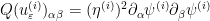
  denotes the usual dot product on . Let us write this equation as

where  is the symmetric tensor

The operator  is a nonlinear differential operator, but it behaves very well with respect to pairing:

We can use (2) to obtain a number of very useful reductions (at the cost of worsening the eventual value of , which as stated in the introduction we will not be attempting to optimise). First we claim that we can drop the injectivity requirement on , that is to say it suffices to show that every Riemannian metric on is of the form  for some map into some Euclidean space . Indeed, suppose that this were the case. Let
  be any (not necessarily isometric) embedding (the existence of which is guaranteed by the Whitney embedding theorem; alternatively, one can use the usual exponential map
  to embed into ). For
  small enough, the map
  is short in the sense that
  pointwise in the sense of symmetric tensors (or equivalently, the map is a contraction from to ). For such an
  , we can write
  for some Riemannian metric . If we then write
  for some (not necessarily injective) map
  , then from (2) we see that
  ; since
  inherits its injectivity from the component map
  , this gives the desired isometric embedding.
Call a metric on good if it is of the form for some map into a Euclidean space . Our task is now to show that every metric is good; the relation (2) tells us that the sum of any two good metrics is good.
In order to make the local theory work later, it will be convenient to introduce the following notion: a map is said to be free if, for every point  , the vectors ,
  and the
  vectors
  ,
,  are all linearly independent; equivalently, given a further map
  , there are no dependencies whatsoever between the
  scalar functions
  , and
, and  , . Clearly, a free map into is only possible for
  , and this explains the bulk of the formula (1) of the best known value of .
For any natural number  , the “Veronese embedding”
  defined by

can easily be verified to be free. From this, one can construct a free map  by starting with an arbitrary immersion
  and composing it with the Veronese embedding (the fact that the composition is free will follow after several applications of the chain rule).
Given a Riemannian metric , one can find a free map which is short in the sense that  , by taking an arbitrary free map and scaling it down by some small scaling factor . This gives us a decomposition

for some Riemannian metric .
The metric is clearly good, so by (2) it would suffice to show that is good. What is easy to show is that is approximately good:
Proposition 5 Let be a Riemannian metric on . Then there exists a smooth symmetric tensor  on with the property that
  is good for every .
Proof: Roughly speaking, the idea here is to use “tightly wound spirals” to capture various “rank one” components of the metric , the point being that if a map “oscillates” at some high frequency  with some “amplitude”
  , then is approximately equal to the rank one tensor
  . The argument here is related to the technique of convex integration, which among other things leads to one way to establish the -principle of Gromov.
By the spectral theorem, every positive definite tensor  can be written as a positive linear combination of symmetric rank one tensors
  for some vector
  . By adding some additional rank one tensors if necessary, one can make this decomposition stable, in the sense that any nearby tensor is also a positive linear combination of the . One can think of
  as the gradient
  of some linear function
  . Using compactness and a smooth partition of unity, one can then arrive at a decomposition
for some finite , some smooth scalar functions  (one can take
  to be linear functions on small coordinate charts, and
  to basically be cutoffs to these charts).
For any and  , consider the “spiral” map
  defined by
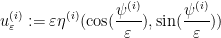
Direct computation shows that

and the claim follows by summing in  (using (2)) and taking
 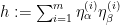 .
.
The claim then reduces to the following local (perturbative) statement, that shows that the property of being good is stable around a free map:
Theorem 6 (Local embedding) Let be a free map. Then  is good for all symmetric tensors sufficiently close to zero in the
  topology.
Indeed, assuming Theorem 6, and with as in Proposition 5, we have  good for small enough. By (2) and Proposition 5, we then have
  good, as required.
The remaining task is to prove Theorem 6. This is a problem in perturbative PDE, to which we now turn.
— 3. Proof of local embedding —
We are given a free map and a small tensor . It will suffice to find a perturbation  of that solves the PDE
We can expand the left-hand side and cancel off to write this as

where the symmetric tensor-valued first-order linear operator  is defined (in terms of the fixed free map ) as

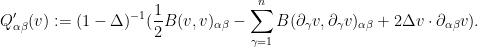
To exploit the free nature of , we would like to write the operator in terms of the inner products and . After some rearranging using the product rule, we arrive at the representation

Among other things, this allows for a way to right-invert the underdetermined linear operator . As is free, we can use Cramer’s rule to find smooth maps  for (with
  ) that is dual to
  in the sense that


where  denotes the Kronecker delta. If one then defines the linear zeroth-order operator from symmetric tensors
  to maps
  by the formula
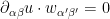
then direct computation shows that  for any sufficiently regular
  . As a consequence of this, one could try to use the ansatz
  and transform the equation (3) to the fixed point equation
One can hope to solve this equation by standard perturbative techniques, such as the inverse function theorem or the contraction mapping theorem, hopefully exploiting the smallness of to obtain the required contraction. Unfortunately we run into a fundamental loss of derivatives problem, in that the quadratic differential operator loses a degree of regularity, and this loss is not recovered by the operator (which has no smoothing properties).
We know of two ways around this difficulty. The original argument of Nash used what is now known as the Nash-Moser iteration scheme to overcome the loss of derivatives by replacing the simple iterative scheme used in the contraction mapping theorem with a much more rapidly convergent scheme that generalises Newton’s method; see this previous blog post for a similar idea. The other way out, due to Gunther, is to observe that  can be factored as

where  is a zeroth order quadratic operator , so that (3) can be written instead as
and using the right-inverse , it now suffices to solve the equation
(compare with (4)), which can be done perturbatively if is indeed zeroth order (e.g. if it is bounded on Hölder spaces such as  ).
).
It remains to achieve the desired factoring (5). We can bilinearise as  , where

The basic point is that when  is much higher frequency than
  , then

which can be approximated by applied to some quantity relating to the vector field  ; similarly if is much higher frequency than . One can formalise these notions of “much higher frequency” using the machinery of paraproducts, but one can proceed in a slightly more elementary fashion by using the Laplacian operator
  and its (modified) inverse operator
  (which is easily defined on the torus using the Fourier transform, and has good smoothing properties) as a substitute for the paraproduct calculus. We begin by writing

The dangerous term here is  . Using the product rule and symmetry, we can write
The second term will be “lower order” in that it only involves second derivatives of , rather than third derivatives. As for the higher order term  , the main contribution will come from the terms where
  is higher frequency than (since the Laplacian accentuates high frequencies and dampens low frequencies, as can be seen by inspecting the Fourier symbol of the Laplacian). As such, we can profitably use the approximation (7) here. Indeed, from the product rule we have

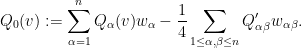
Putting all this together, we obtain the decomposition

where

and
If we then use Cramer’s rule to create smooth functions  dual to the
  in the sense that

then we obtain the desired factorisation (5) with
Note that  is the smoothing operator applied to quadratic expressions of up to two derivatives of . As such, one can show using elliptic (Schauder) estimates to show that is Lipschitz continuous in the Holder spaces
  for
for  (with the Lipschitz constant being small when has small norm); this together with the contraction mapping theorem in the Banach space is already enough to solve the equation (6) in this space if is small enough. This is not quite enough because we also need to be smooth; but it is possible (using Schauder estimates and product Hölder estimates) to establish bounds of the form

for any  (with implied constants depending on
  but independent of
  ), which can be used (for small enough) to show that the solution constructed by the contraction mapping principle lies in
  for any (by showing that the iterates used in the construction remain bounded in these norms), and is thus smooth.


29 comments
Comments feed for this article
12 May, 2016 at 12:43 am
Bo Jacoby
Does theorem 2 imply that space-time around a star can be imbedded in some higher dimensional euclidean space?
12 May, 2016 at 8:29 am
Terence Tao
Spacetime is pseudo-Riemannian rather than Riemannian, and so cannot be embedded in any Riemannian space. I guess the natural conjecture would be that a -dimensional spacetime may be locally isometrically embedded into some high dimensional Minkowski spacetime, but I don’t know if there are such results in the literature. (Global embedding is unrealistic because the spacetime may contain causal loops, which Minkowski spacetime, which of course doesn’t have any.) There are at least two obstacles to extending the arguments in this post to the pseudo-Riemannian setting: firstly, the Cartesian product of two Minkowski spacetimes is not a Minkowski spacetime, making the pairing operation much less useful; and secondly, the d’Lambertian (the natural analogue of the Laplacian in this setting) is no longer elliptic. But the latter obstacle at least might still be manageable using the original Nash-Moser method, which can tolerate some loss of derivatives in the nonlinearity.
12 May, 2016 at 9:59 am
Harshvardhan Tandon
Sir I am a high school student and a big fan of yours. I was a bit curious regarding your thoughts about the hotly debated ABC conjecture(about which I believe you must have given some thought). So what do you think about the enormous proof posed by Shinichi Mochizuki?Is it anywhere close to being correct or is it just a pointless and confusing pursuit which will not lead to anything important?
12 May, 2016 at 1:38 pm
Terence Tao
This recent post by Brian Conrad is probably the best summary of the current state of affairs: https://mathbabe.org/2015/12/15/notes-on-the-oxford-iut-workshop-by-brian-conrad/
26 August, 2016 at 12:35 am
Olaf Müller
Fortunately, your conjecture has a positive answer Miguel Sánchez and I found some years ago:
https://arxiv.org/abs/0812.4439
As you say, noncausality is an obstruction to the existence of an isometric embedding into a Minkowski space-time. An equivalent characterization for the existence is the existence of a steep temporal function, i.e. a function whose gradient v satisfies g(v,v) <-1, and such a function exists in every globally hyperbolic space-time. (If we asked for a conformal embedding instead of an isometric one, then the embeddable space-times would be exactly the stably causal ones.)
Now, if we focus on the local question, then we can use that in every space-time, every point has a globally hyperbolic neighborhood, thus, indeed, the local question is unobstructed.
Best,
-olaf.
18 August, 2020 at 10:26 am
rogerwest
What is meant by “causal” here? And why does it surface here, while the main article doesn’t allude to it?
20 August, 2020 at 2:19 pm
Terence Tao
Lorenztial spacetimes have causal structure, but Riemannian manifolds (the focus of the main article) do not.
13 May, 2016 at 12:44 pm
lewallen
Thanks a lot for the notes, great reading. I was a bit confused early on until I realized that by “pairing” two functions you meant the cartesian product (is that right?) — I’d never seen that particular terminology. What do you think about making that more explicit (e.g. in the proof of the Whitney immersion theorem)?
13 May, 2016 at 12:48 pm
lewallen
hah I just noticed that you explicitly defined it in the introduction, in fact it’s a central technique is you point out ;). Ok, sorry about that!
14 May, 2016 at 2:15 am
Paul Bryan
The paragraph on upgrading the weak Whitney theorem to an embedding is a little unclear. The immersion is locally an embedding, so is injective in a neighbourhood of any point. The statement, “if
  , then
  is injective on a neighbourhood of
  …” is thus a little odd. It may also be helpful to remark that, although an injective immersion is not in general an embedding, for
  compact, it is since any continuous bijection from a compact space to a Hausdorff space is a homeomorphism.
[Text modified, thanks – T.]
14 May, 2016 at 8:08 pm
Anonymous
nice
15 May, 2016 at 10:32 pm
Notes on the Nash embedding theorem — What’s new | wendaliblog
[…] via Notes on the Nash embedding theorem — What’s new […]
17 May, 2016 at 11:32 am
Luiz Botelho -Físico Matemático de Altas energias e Turbulencia estocástica.
Terence
Beautiful argument .I think it can work for sigma compact Riemannian Manifolds .Relate to the General Relativity Problem , it is usual to postulate that you can complexify your pseudo Riemann manifold to a Complex Manifold with a Complex bilinear form as the Riemanian metric ,if this makes sense at all and thus apply Nash theorem for the Euclidean Manifold section (Now a truly Rieman Manifold!) .Any chance to extend this result by analytic continuation to the whole , now a complex manifold ?.Of course that some deep topological restrictions must be imposed , like Manifold Global orientability (By the way , if you consider orientability -Global , can this simplifies the Theorem ?).Being a spin manifold , etc….
18 September, 2016 at 7:21 pm
Hu
there is a very very little mistake with symbol:
Call a metric {g} on {({\bf R}/{\bf Z})^d} good if it is of the form {Q(u)} for some map {u: ({\bf R}/{\bf Z})^n \rightarrow {\bf R}^d} into a Euclidean space {{\bf R}^d}. Our task is now to show that every metric is good; the relation (2) tells us that the sum of any two good metrics is good.
{({\bf R}/{\bf Z})^d} should be {({\bf R}/{\bf Z})^n}
[Corrected, thanks – T.]
27 November, 2016 at 8:19 am
haduonght
Reblogged this on Eniod's Blog and commented:
Terence Tao notes on embedding theorem.
26 November, 2018 at 9:27 am
Embedding the Heisenberg group into a bounded dimensional Euclidean space with optimal distortion | What's new
[…] has some formal similarities with the isometric embedding problem (discussed for instance in this previous post), which can be viewed as the problem of solving an equation of the form , where is a Riemannian […]
8 January, 2019 at 3:12 pm
255B, Notes 2: Onsager’s conjecture | What's new
[…] is a celebrated theorem of Nash (discussed in this previous blog post) that the isometric embedding problem is possible in the smooth category if the dimension is large […]
15 February, 2019 at 1:36 am
maria
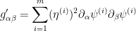
Professor Tao, could you maybe explain the decomposition of g_{\alpha,\beta} in the proof of proposition 5? As far as I understand, one can write a symmetric positive definite matrix as a product V^T\times V where the rows of V are the eigenvectors of the matrix multiplied by the square root of the positive eigenvalues. Hence, if \psi(x)=V\times x, then g_{\alpha,\beta}is given by the inner product of \partial_\alpha \psi and \partial_\beta \psi.
15 February, 2019 at 2:27 pm
Terence Tao
This gives the required decomposition at a single point . To make a decomposition that applies for an open set of
  one needs a more stable decomposition than the spectral decomposition; see Lemma 16 of my more recent notes https://terrytao.wordpress.com/2019/01/08/255b-notes-2-onsagers-conjecture/ for details.
15 February, 2020 at 8:36 pm
Brian
I notice that both arguments of the max operator are second degree polynomials. A gross but true overestimate then for the d in Nash’s embedding theorem would be, for large enough n, n^3.
In fact, it seems 3 is the minimum of k such that n^k (the monomial) is a bound for d for all n after a certain point.
Why is this? I guess another way to ask is why is the bound Gunther found second degree? Why not first, third, or more than third?
16 February, 2020 at 10:06 am
Terence Tao
Well, the equation is
is  distinct equations in
  unknowns, so one should certainly expect smooth embedding to only be possible for
  (this can be made rigorous by computing the dimension of the image of the Taylor coefficients at the origin of
  up to some large order as $u$ varies over smooth maps, and comparing this with the dimension of the space of Taylor coefficients of
  ; I give an argument of this form for instance in Section 3 of https://arxiv.org/abs/1902.06313 ).
The main constraint in the known arguments for Nash embedding require one to begin with a smooth (but not isometric) embedding which is free in the sense that the first derivatives
  and the second derivatives
  are linearly independent (after taking into account the obvious symmetry
  . This forces
 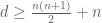 at a bare minimum. It remains an open question what the precise optimal dependence on
  and
and  is.
is.
6 March, 2020 at 7:34 pm
Anonymous
After (5), it states “ ”. Isn’t the sign off? In other words, should it not be “
 ”? Also, later there is a definition of “
 ” Surely this must be
  .
.
[Corrected, thanks – T.]
28 March, 2020 at 5:06 pm
Martin Ondrejat
Concerning the smoothness of the solution (the final step) the proof seems to be using uniform boundedness of the operator norms of from
from  to
to  with respect to all
  positive. Is this really true? If one realizes that the number of derivatives of
  -th order does not increase in
  linearly, this would be surprising to hold …
29 March, 2020 at 7:48 am
Terence Tao
The operator commutes with all constant coefficient differential operators, and in particular with
  . Because of this, once one knows that
  maps
maps  to
to  , it is immediate that it also maps
  to
to  . (To put it another way: the operator
  is a Fourier multiplier and thus does not change the frequency of the function it is applied to, only the amplitude. Varying the regularity exponent in Holder or Sobolev norms such as
  corresponds to multiplying the norm by some power of the frequency (at least for functions that are localised to a single frequency annulus). If the frequency doesn’t change, then this makes the
  norm effectively a scalar multiple of the norm
  for the function, and
  the same scalar multiple of
  of the output, so the effect of increasing $k$ on both sides cancels out.)
29 March, 2020 at 11:04 am
Martin Ondrejat
I can see that what you write works in the scale of the Sobolev spaces W^{k,2} (because there, everything can be transfered to the language of coordinates with respect to the orthonormal basis). And it is actually sufficient for the proof. One does not even need the (difficult) Schauder estimates for C^{k,\alpha} which can be replaced by (easy) estimates in the Sobolev W^{k,2} spaces (which are also an algebra for large k). And then the proof is really simple. Great!
30 August, 2020 at 12:27 pm
James Green
Hello,
I went to read the proof of the Nash Embedding theorem after I read your notes above. When you mention ” loss of derivatives problem” is this overcome in the original proof , by Nash, by using mollification in the convolution in Nash’s paper?
30 August, 2020 at 1:13 pm
Anonymous
Yes.
3 January, 2021 at 11:50 am
Anonymous
Can you comment on paraproduct machinery?
8 January, 2021 at 8:43 pm
Anonymous
In the formula after “If we then use Cramer’s rule to create smooth functions”, should it be delta_{…} instead of 0?
[No. One could augment the to a more complete dual basis by also locating vectors
  that are dual to the
  , but these are not necessary for this argument. -T]