
We consider the incompressible Euler equations on the (Eulerian) torus 


As noted previously, the kinetic energy
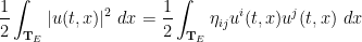
 is the Euclidean metric. Indeed, if one assumes that
  are continuously differentiable in both space and time on
 ![{[0,T] \times \mathbf{T}}](https://s0.wp.com/latex.php?latex=%7B%5B0%2CT%5D+%5Ctimes+%5Cmathbf%7BT%7D%7D&bg=ffffff&fg=000000&s=0&c=20201002) , then one can multiply the equation (1) by
, then one can multiply the equation (1) by  and contract against
  to obtain
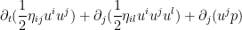
![{[0,T] \times \mathbf{T}_E}](https://s0.wp.com/latex.php?latex=%7B%5B0%2CT%5D+%5Ctimes+%5Cmathbf%7BT%7D_E%7D&bg=ffffff&fg=000000&s=0&c=20201002) and uses Stokes’ theorem, one obtains the required energy conservation law
and uses Stokes’ theorem, one obtains the required energy conservation law 
 is not a test function and so one cannot immediately integrate (1) against . And indeed, as we shall soon see, it is now known that once the regularity of
  is low enough, energy can “escape to frequency infinity”, leading to failure of the energy conservation law, a phenomenon known in physics as anomalous energy dissipation.
But what is the precise level of regularity needed in order to for this anomalous energy dissipation to occur? To make this question precise, we need a quantitative notion of regularity. One such measure is given by the Hölder space 


 lies between the space
  of continuous functions and the space
  of continuously differentiable functions, and informally describes a space of functions that is “
 times differentiable” in some sense. The above derivation of the energy conservation law involved the integral
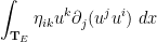
 once
once  . More precisely, one can make
Conjecture 1 (Onsager’s conjecture) Let, and let
.
- (i) If
to the Euler equations (in the Leray form
) obeys the energy conservation law (3).
- (ii) If
, then there exist weak solutions
This conjecture was originally arrived at by Onsager by a somewhat different heuristic derivation; see Remark 7. The numerology is also compatible with that arising from the Kolmogorov theory of turbulence (discussed in this previous post), but we will not discuss this interesting connection further here.
The positive part (i) of Onsager conjecture was established by Constantin, E, and Titi, building upon earlier partial results by Eyink; the proof is a relatively straightforward application of Littlewood-Paley theory, and they were also able to work in larger function spaces than 


In these notes we will first establish (i), then discuss the convex integration method in the original context of the Nash-Kuiper embedding theorem. Before tackling the Onsager conjecture (ii) directly, we discuss a related construction of high-dimensional weak solutions in the Sobolev space 


We thank Phil Isett for some comments and corrections.
— 1. Energy conservation for sufficiently regular weak solutions —
We now prove the positive part (i) of Onsager’s conjecture, which turns out to be a straightforward application of Littlewood-Paley theory. We need the following relation between Hölder spaces and Littlewood-Paley projections:
Exercise 2 Letfor some
. Establish the bounds

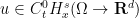
Let ![{u \in C^0_t C^{0,\alpha}([0,T] \times \mathbf{T}_E \rightarrow {\bf R})}](https://s0.wp.com/latex.php?latex=%7Bu+%5Cin+C%5E0_t+C%5E%7B0%2C%5Calpha%7D%28%5B0%2CT%5D+%5Ctimes+%5Cmathbf%7BT%7D_E+%5Crightarrow+%7B%5Cbf+R%7D%29%7D&bg=ffffff&fg=000000&s=0&c=20201002)


 . Applying
  to (4), we have
 , and thus
  . Thus
  solves the PDE


 onto the divergence-free factor , at which point it may be removed. Moving the derivative
  over there as well, we now reduce to showing that
 is a total derivative (as is divergence-free), and thus has vanishing integral. Thus it will remain to show that
 ![\displaystyle \int_0^T \int_{\mathbf{T}_E} \partial_j P_{\leq N} u \cdot [ P_{\leq N} (u^j u) - P_{\leq N} u^j P_{\leq N} u] dx dt = o(1).](https://s0.wp.com/latex.php?latex=%5Cdisplaystyle+%5Cint_0%5ET+%5Cint_%7B%5Cmathbf%7BT%7D_E%7D+%5Cpartial_j+P_%7B%5Cleq+N%7D+u+%5Ccdot+%5B+P_%7B%5Cleq+N%7D+%28u%5Ej+u%29+-+P_%7B%5Cleq+N%7D+u%5Ej+P_%7B%5Cleq+N%7D+u%5D+dx+dt+%3D+o%281%29.&bg=ffffff&fg=000000&s=0&c=20201002)
 that
that 
 is finite, it thus suffices to establish the pointwise bound


 .
.
To treat (7), we use Exercise 2 to conclude that
 , which is acceptable since . Now we turn to (5). This is a commutator of the form
 . Observe that this commutator would vanish if were replaced by
  , thus we may write this commutator as
 . If we write
 of total mass one, we have

 , we thus have the bound

 , which is acceptable since . A similar argument gives (6), and the claim follows.
As shown by Constantin, E, and Titi, the Hölder regularity in the above result can be relaxed to Besov regularity, at least in non-endpoint cases:
Exercise 3 Letto be the space of functions
such that the Besov space norm
Show that if
is a weak solution to the Euler equations, the energy
is conserved in time.

The endpoint case 

As observed by Isett (see also the recent paper of Colombo and de Rosa), the above arguments also give some partial information about the energy in the low regularity regime:
Exercise 4 Let
- (i) If
is a
.)
- (ii) If
, show that the energy
function of time.
Exercise 5 Let. Establish the energy identity

Remark 6 An alternate heuristic derivation of the, then from Exercise 2 we see that the portion of
has amplitude
at most
; in particular, the amount of energy at frequencies
is at most
. On the other hand, by the heuristics in Remark 11 of 254A Notes 3, the time
needed for the portion of the solution at frequency
is of order
. Thus the rate of energy flux at frequency
. For
, the energy flux goes to zero as
Remark 7 Yet another alternate heuristic derivation of thethe Euler equations may be written as
In particular, the energy
at a single Fourier mode
evolves according to the equation
If
for any
, hence by Plancherel’s theorem
which suggests that (up to logarithmic factors) one would expect
to be of magnitude about
. Onsager posited that for typically “turbulent” or “chaotic” flows, the main contributions to (8) come when
have magnitude roughly comparable to that of
, one might expect about
significant terms in the sum, which according to standard “square root cancellation heuristics” (cf. the central limit theorem) suggests that the sum is about as large as
times the main term. Thus the total flux of energy in or out of a single mode
, and so the total flux in or out of the frequency range
(which consists of
modes
. As such, for
threshold by a more physical space based approach, a rigorous version of which was eventually established by Duchon and Robert; see this survey of Eyink and Sreenivasan for more discussion.


— 2. The (local) isometric embedding problem —
Before we develop the convex integration method for fluid equations, we first discuss the simpler (and historically earlier) instance of this technique for the isometric embedding problem for Riemannian manifolds. To avoid some topological technicalities that are not the focus of the present set of notes, we only consider the local problem of embedding a small neighbourhood 


Let 


The isometric embedding problem asks, given a Riemannian manifold such as 


It is a celebrated theorem of Nash (discussed in this previous blog post) that the isometric embedding problem is possible in the smooth category if the dimension 
Theorem 8 (Nash embedding theorem) Suppose that. Then for any smooth metric
on some smaller neighbourhood
of the origin.
The optimal value of
 below
below  :
:
Proposition 9 Suppose that. Then there exists a smooth Riemannian metric
Proof: Informally, the reason for this is that the given field 


 of the Euclidean metric
  on
on  (here it is important to restrict to
  in order to avoid the symmetry constraint
  ; also, the positive definiteness of the metric will be automatic as long as one restricts to sufficiently small perturbations). Comparing dimensions, we conclude that if every smooth metric had a smooth embedding , one must have the inequality
 and sending , we conclude that
  . Taking contrapositives, the claim follows.
Remark 10 If one replaces “smooth” with “analytic”, one can reverse the arguments here using the Cauchy-Kowaleski theorem and show that any analytic metric on; this is a classical result of Cartan and Janet.
Apart from the slight gap in dimensions, this would seem to settle the question of when a 
It is a remarkable (and somewhat counter-intuitive) result of Nash and Kuiper that if one only requires the embedding to be in
Theorem 11 (Nash-Kuiper embedding theorem) Let. Then for any smooth metric
Nash originally proved this theorem with the slightly weaker condition 


Remark 12 One striking illustration of the distinction between the(with the usual metric) into Euclidean space
. It is a classical result (see e.g., Spivak’s book) that the only
isometric embeddings of
with an isometry of the Euclidean space; however, the Nash-Kuiper construction allows one to create an
To prove this theorem we work with a relaxation of the isometric embedding problem. We say that 


Proposition 13 Let, and let
.
Proof: Set 


To create a true isometric embedding 


We now prove Theorem 11. The key iterative step is
Theorem 14 (Iterative step) Letbe a closed ball in
, one can find a short isometric embedding
to (11) on


Suppose for the moment that we had Theorem 14. Starting with the short isometric embedding 


 . From this we see that
  converges uniformly to zero, while
  converges in norm to a limit , which then solves (10) on , giving Theorem 11. (Indeed, this shows that the space of isometric embeddings is dense in the space of short maps in the topology.)
We prove Theorem 14 through a sequence of reductions. Firstly, we can rearrange it slightly:
Theorem 15 (Iterative step, again) Letbe a smooth immersion, and let
be a smooth Riemannian metric on
of smooth immersions for
obeying the bounds
uniformly on
denotes a quantity that goes to zero as
).


Let us see how Theorem 15 implies Theorem 14. Let the notation and hypotheses be as in Theorem 14. We may assume 


 is smooth, symmetric, and (from (13)) will be positive definite for large enough. By construction, we thus have
  solving (11), and Theorem 14 follows.
To prove Theorem 15, it is convenient to break up the metric
Lemma 16 (Rank one decomposition) Letof unit vectors
in
, such that
for all
. Furthermore, for each
of the
are non-zero.
Remark 17 Strictly speaking, the unit vectorsshould belong to the dual space
of
appear as subscripts instead of superscripts. A similar consideration occurs for the frequency vectors
from Remark 7. However, we will not bother to distinguish between
Proof: Fix a point 


 , where are the
  unit vectors of the form
  for
for  , enumerated in an arbitrary order. From the further parallelogram identity

 also has a representation of the form (14) with slightly different coefficients
  that depend smoothly on the perturbation. As is smooth, we thus see that for
  sufficiently close to we have the decomposition
 varying smoothly with . This gives the lemma in a small ball
  centred at ; the claim then follows by covering by a finite number balls of the form
  (say), covering these balls by balls
  of a fixed radius
  smaller than all the
  in the finite cover, in such a way that any point lies in at most of the balls
  , constructing a smooth partition of unity
  adapted to the , multiplying each of the decompositions of
  previously obtained on
  (which each lie in one of the ) by
  , and summing to obtain the required decomposition on .
Remark 18 Informally, Lemma 16 lets one synthesize a metric-principle“, which we will not discuss further here.
One can now deduce Theorem 15 from
Theorem 19 (Iterative step, rank one version) Letbe a unit vector, and let
be smooth. Then there exists a sequence
uniformly on
is contained in the support of
.


Indeed, suppose that Theorem 19 holds, and we are in the situation of Theorem 15. We apply Lemma 16 to obtain the decomposition
 . Applying Theorem 19
  times (and diagonalising the sequences as necessary), we obtain sequences
  of smooth immersions for
  such that
  and one has


 is contained in that of . The claim then follows from the triangle inequality, noting that the implied constant in (12) will not depend on because of the bounded overlap in the supports of the .
It remains to prove Theorem 19. We note that the requirement that 


Writing 


To locate these functions 


 is a smooth function independent of to be chosen later; thus is a function both of the “slow” variable and the “fast” variable
  taking values in the“fast torus”
  . (We adopt the convention here of using boldface symbols to denote functions of both the fast and slow variables. The fast torus is isomorphic to the Eulerian torus
  from the introduction, but we denote them by slightly different notation as they play different roles.) Thus is a low amplitude but highly oscillating perturbation to . The fast variable oscillation means that will not be bounded in regularity norms higher than (and so this ansatz is not available for use in the smooth embedding problem), but because we only wish to control and type quantities, we will still be able to get adequate bounds for the purposes of embedding. Now that we have twice as many variables, the problem becomes more “underdetermined” and we can arrive at a simpler PDE by decoupling the role of the various variables (in particular, we will often work with PDE where the derivatives of the main terms are in the fast variables, but the coefficients only depend on the slow variables, and are thus effectively constant coefficient with respect to the fast variables).
Remark 20 Informally, one should think of functionsthat are independent of the fast variable
as being of “low frequency”, and conversely functions that have mean zero in the fast variable
for all
can be uniquely decomposed into a “low frequency” component and a “high frequency” component, with the two components orthogonal to each other. In later sections we will start inverting “fast derivatives”
on “high frequency” functions, which will effectively gain important factors of
in the analysis. See also the table below for the dictionary between ordinary physical coordinates and fast-slow coordinates.
| Position | Slow variable |
Fast variable  | Fast variable  |
Function  | Function  |
 |  |
Low-frequency function  | Function independent of |
| High-frequency function | Function mean zero in |
| N/A | Slow derivative |
| N/A | Fast derivative  |
If we expand out using the chain rule, using 


 were unit vectors varying smoothly with respect to the slow variable; this obeys (22) and (19), and would also obey (21) if the vectors
  and
and  were both always orthogonal to the entire gradient of . This is not possible in
  (as cannot then support
  linearly independent vectors), but there is no obstruction for :
Lemma 21 (Constructing an orthogonal frame) Letare unit vectors orthogonal to each other and to
for
Proof: Applying the Gram-Schmidt process to the linearly independent vectors 


For 


 smoothly to this segment with the specified initial data at , and a simple calculation using Gronwall’s inequality shows that the system of equations (23), (24), (25) is preserved by this evolution. Then, one can extend to the disk
  by using the previous extension to the segment as initial data and solving the parallel transport ODE
This concludes Nash’s proof of Theorem 11 when 


 , one is reduced to locating such functions
  that obey the bounds

This can be done by an explicit construction:
Exercise 22 (One-dimensional corrugation) For any positiveand any
, show that there exist smooth functions
solving the ODE
and which vary smoothly with
(even at the endpoint
), and obey the bounds
(Hint: one can renormalise
. The problem is basically to locate a periodic function
mapping
to the circle
of mean zero and Lipschitz norm
that varies smoothly with
for some smooth and small
that is even and compactly supported in
with mean zero on each interval, and then choose
to be odd.)


This exercise supplies the required functions
Remark 23 For sake of discussion let us restrict attention to the surface case. For the local isometric embedding problem, we have seen that we have rigidity at regularities at or above
level for
, while a result of de Lellis, Inauen, and Szekelyhidi (building upon a series of previous results) establishes non-rigidity when
. For recent results in higher dimensions, see this paper of Cao and Szekelyhidi.
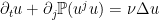
— 3. Low regularity weak solutions to Navier-Stokes in high dimensions —
We now turn to constructing solutions (or near-solutions) to the Euler and Navier-Stokes equations. For minor technical reasons it is convenient to work with solutions that are periodic in both space and time, and normalised to have zero mean at every time (although the latter restriction is not essential for our arguments, since one can always reduce to this case after a Galilean transformation as in 254A Notes 1). Accordingly, let 

 denote the space of smooth periodic functions
  that have mean zero and are divergence-free at every time
  , thus

 as an abbreviation for
  for various vector spaces
  (the choice of which will be clear from context).
Let 


 and smooth
  . Here of course
  denotes the spatial Laplacian.
Much as we replaced the equation (10) in the previous section with (11), we will consider the relaxed version 


Note that if 


It will be thus of interest to find, for a given 


To execute above strategy, it will be convenient to have an even more flexible notion of solution, in which 


If the error terms 

Exercise 24 (Removing the error terms) Let
and
is the mean of
(Hint: one will need at some point to show that
has mean zero in space at every time; this can be achieved by integrating (32) in space.)


Because of this exercise we will be able to tolerate the error terms 
As a simple corollary of Exercise 24, we have the following analogue of Proposition 13:
Proposition 25 Letfor some compact time interval
, then
can be chosen to also be supported in this region.
Proof: Clearly 

 at , which then verifies the claimed properties.
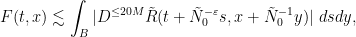
Now, we show that, in sufficiently high dimension, a Navier-Stokes-Reynolds flow 


Proposition 26 (Weak improvement of Navier-Stokes-Reynolds flows) Letbe a Navier-Stokes-Reynolds flow. Then for sufficiently large
obeying the estimates
for all
, and such that
Furthermore, if
for some interval
, then one can arrange for
to be supported on
for any interval
containing
).


This proposition can be viewed as an analogue of Theorem 14. For an application at the end of this section it is important that the implied constant in (36) is uniform in the choice of initial flow 


To simplify the notation we adopt the following conventions. Given an 


 . Informally, one should read the above estimate as asserting that is bounded in with norm
  , and oscillates with frequency
  in time and in space (or equivalently, with a temporal wavelength of
  and a spatial wavelength of
  ).
).
Proof: We can assume that 

Assume

 at supported on
  and obeying the bounds

 .
.
It will in fact suffice to construct an approximate difference Navier-Stokes-Reynolds flow 


To construct this approximate solution, we again use the method of fast and slow variables. Set 


 as a “low-frequency” function (in the sense of Remark 20) that only depends on and the slow variable , but not on the fast variable .
Let 


 , and similarly for (48), (49). (Note here that there was considerable room in the estimates with regards to regularity in the variable; this room will be exploited more in the next section.) For any shift
  , we see from the chain rule that
  is an approximate difference Navier-Stokes-Reynolds flow at supported on , where


 . By Markov’s inequality and (52), we see that for each
  , we have
 outside of an exceptional set of measure (say)
  . Similarly for the other equations above. Applying the union bound, we can then find a such that obeys all the required bounds (37)–(41) simultaneously for all . (This is an example of the probabilistic method, originally developed in combinatorics; one can think of probabilistically as a shift drawn uniformly at random from the torus , in order to relate the fast-slow Lebesgue norms to the original Lebesgue norms .)
It remains to construct an approximate fast-slow solution 


Now we need to construct a simplified fast-slow solution 


We turn to the details. Our preliminary construction of the velocity field 
Exercise 27 Letmatrices
. Show that there exist non-zero lattice vectors
and smooth functions
for some
such that
for all
. (This decomposition is essentially due to de Lellis and Szekelyhidi. The subscripting and superscripting here is reversed from that in Lemma 16; this is because we are now trying to decompose a rank

We would like to apply this exercise to the matrix with entries 

 is the Frobenius norm of
  . Then is smooth and is positive definite on all of the compact spacetime (recall that we can assume to not be identically zero), and in particular ranges in a compact subset of positive definite matrices. Applying the previous exercise and composing with the function
  , we conclude that there exist non-zero lattice vectors and smooth functions
  for some such that
 . As
. As  depend only on
  , and is a component of , all norms of these quantities are bounded by
  ; they are independent of . Furthermore, on taking traces and integrating on , we obtain the estimate
  , ). By applying a smooth cutoff
  in time that equals
  on and vanishes outside of to
  (and applying
  to ), we may assume that the are supported in ; this redefines slightly to
Now for each 


Let 


 of
of  is also not identically zero (thanks to the unique continuation property of harmonic functions). We can normalise so that
 (basically by first constructing a version of on a standard cylinder
  and the applying an affine transformation to map onto ).
Let 
 , with the presence of the Laplacian
  ensuring that this function is extremely well balanced (for instance, it will have mean zero, and thus “high frequency” in the sense of Remark 20). Clearly
  is divergence free, and one also has the steady-state Euler equation

 and
and  . If we then set

 is a simplified fast-slow solution supported in . Direct calculation using the Leibniz rule then gives the bounds

 , while from (64) one has
  ).
).
This looks worse than (56)–(60). However, observe that 


We are now a bit closer to (56)–(60), but our bounds on 

 is supported on
  and obeys the estimates
  . Observe that
 as
as  . Iterating the above identity times, we obtain


 is supported in . Observe that
  is a simplified fast-slow solution supported in , where

 large enough
  . Meanwhile, another appeal to (72) yields
  , and hence by (67) and the triangle inequality

 continues to be supported on the thin set , we can apply Hölder as before to conclude that
  . Also, from (73) and Hölder we have
We have now achieved the bound (59); the remaining estimate that needs to be corrected for is (60). This we can do by a modification of the previous argument, where we now work to reduce the size of


 is the linear operator on smooth vector-valued functions on of mean zero defined by the formula
 also has mean zero. We can thus iterate and obtain

 is a smooth function whose exact form is explicit but irrelevant for our argument. We then see that
  is a simplified fast-slow solution supported in
  . Since
  is bounded in
  , we see from (69) that
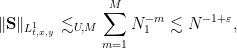
 is large enough. Thus obeys the required bounds (56)–(60), concluding the proof.
As an application of this proposition we construct a low-regularity weak solution to high-dimensional Navier-Stokes that does not obey energy conservation. More precisely, for any 


 on functions in a distributional sense, basically because the adjoint operator
  maps test functions to bounded functions.)
Corollary 28 (Low regularity non-trivial weak solutions) Assume that the dimensionsolution
, but is not identically zero. In particular, periodic weak

Proof: Let 

![{[0.4, 0.6] \times \mathbf{T}_E}](https://s0.wp.com/latex.php?latex=%7B%5B0.4%2C+0.6%5D+%5Ctimes+%5Cmathbf%7BT%7D_E%7D&bg=ffffff&fg=000000&s=0&c=20201002)


![{[0.3 + 2^{-n}/100, 0.7 - 2^{-n}/100] \times \mathbf{T}_E}](https://s0.wp.com/latex.php?latex=%7B%5B0.3+%2B+2%5E%7B-n%7D%2F100%2C+0.7+-+2%5E%7B-n%7D%2F100%5D+%5Ctimes+%5Cmathbf%7BT%7D_E%7D&bg=ffffff&fg=000000&s=0&c=20201002)


 . For
. For  sufficiently rapidly growing, this implies that
  converges strongly in to zero, while
  converges strongly in to some limit
  supported in
 ![{[0.3, 0.7] \times \mathbf{T}_E}](https://s0.wp.com/latex.php?latex=%7B%5B0.3%2C+0.7%5D+%5Ctimes+%5Cmathbf%7BT%7D_E%7D&bg=ffffff&fg=000000&s=0&c=20201002) . From the triangle inequality we have
. From the triangle inequality we have  is sufficiently rapidly growing) and hence is not identically zero if is chosen large enough. Applying Leray projections to the Navier-Stokes-Reynolds equation we have
 is the vector field with components
  for ); taking distributional limits as
  , we conclude that is a periodic weak solution to the Navier-Stokes equations, as required.
— 4. High regularity weak solutions to Navier-Stokes in high dimensions —
Now we refine the above arguments to give a higher regularity version of Corollary 28, in which we can give the weak solutions almost half a derivative of regularity in the Sobolev scale:
Theorem 29 (Non-trivial weak solutions) Let, and assume that the dimension
This result is inspired by a three-dimensional result of Buckmaster and Vicol (with a small value of 


In the proof of Corollary 28, we took the frequency scales 
We turn to the details. We select the following parameters:
- A regularity
- A quantity
- An integer
, assumed to be sufficiently large depending on
; and
- A dimension
.
 . To simplify the notation we allow all implied constants to depend on
  unless otherwise specified. We recall from the previous section the notion of a Navier-Stokes-Reynolds flow . The basic strategy is to start with a Navier-Stokes-Reynolds flow and repeatedly adjust by increasingly high frequency corrections in order to significantly reduce the size of the stress (at the cost of making both of these expressions higher in frequency).
As before, we abbreviate 

The main iterative statement (analogous to Theorem 14) starts with a Navier-Stokes-Reynolds flow 


Theorem 30 (Iterative step) Let. Suppose that one has a Navier-Stokes-Reynolds flow
obeying the estimates
for some
. Set
. Then there exists a Navier-Stokes-Reynolds flow
obeying the estimates
Furthermore, if
is supported in
-neighbourhood of


Let us assume Theorem 30 for the moment and establish Theorem 29. Let 
![{[0.4,0.6] \times \mathbf{T}_E}](https://s0.wp.com/latex.php?latex=%7B%5B0.4%2C0.6%5D+%5Ctimes+%5Cmathbf%7BT%7D_E%7D&bg=ffffff&fg=000000&s=0&c=20201002)


 . In particular, the
  converge weakly to zero on , and we have the bound

 converges strongly in
  (and in particular also in
  for some
  ) to some limit
  ; as the are all divergence-free, is also. From applying Leray projections to (26) one has
  is a weak solution to Navier-Stokes. Also, from construction one has
  large enough is not identically zero. This proves Theorem 29.
It remains to establish Theorem 30. It will be convenient to introduce the intermediate frequency scales

 , and
, and  (and constrained to be integer).
Before we begin the rigorous argument, we first give a heuristic explanation of the numerology. The initial solution 


 , this is slightly less than
  , allowing one to close the argument.
We now turn to the rigorous details. In a later part of the argument we will encounter a loss of derivatives, in that the new Navier-Stokes-Reynolds flow
Proposition 31 (Mollification) Let the notation and hypotheses be as above. Then we can find a Navier-Stokes-Reynolds flowobeying the estimates
and
for all
and
Furthermore, if
is supported in
, where
is the
-neighbourhood of


We remark that this sort of mollification step is now a standard technique in any iteration scheme that involves loss of derivatives, including the Nash-Moser iteration scheme that was first used to prove Theorem 8.
Proof: Let 


 is the identity operator and
 and
and  will behave like low and high frequency Littlewood-Paley projections. (We cannot directly use these projections here because their convolution kernels are not localised in time.)
Observe that 


 ,
,  is a linear combination of the operators
  . In particular, we see that is supported on
  .
.
We abbreviate 


 , thanks to Young’s inequality. A similar application of Young’s inequality gives
  and .
and .
From (81) and decomposing 

 , and hence (77) follows from (75). In a similar spirit, from (82), (75) one has


 is large enough; similar arguments give the same bound if
  is deleted. This gives (79), (80).
Finally we prove (78). By the triangle inequality it suffices to show that 


 by
by  ) this is bounded by
 . For
. For  , we rewrite the expression

 ) by
) by  by , and (75) is bounded by
  is large. The other terms are treated similarly.
We return to the proof of Theorem 30. We abbreviate 


 at supported on , obeying the estimates


 to the difference equation at supported on supported in obeying the bounds (86), (88), (89)
Now, we pass to fast and slow variables. Let 
 is consistent with oscillations in time of wavelength
  , in the slow variable of wavelength
  , and in the fast variable of wavelength
  .
.
Exercise 32 By using the method of fast and slow variables as in the previous section, show that to construct the approximate Navier-Stokes-Reynolds flowrather than


As in the previous section, we can then pass to simplified fast-slow soutions:
Exercise 33 Show that to construct the approximate fast-slow solution(Hint: one will need the estimate
from Proposition 31.)


Now we need to construct a simplified fast-slow solution 

As before, we need to select 

Lemma 34 (Smooth polar-type decomposition) There exists a factorisation, where
,


Proof: We may assume that 


 , so we apply a smoothing operator. Let
  denote the function
 , then by Fubini’s theorem (or Young’s inequality)
 is smooth and strictly positive everywhere, and from differentation under the integral sign and integration by parts we have
 . Also, from construction one has

 . From many applications of the chain rule (or the Faá di Bruno formula), we see that for any
  ,
,  is a linear combination of
  terms of the form
 sum up to (more precisely, each component of
  is a linear combination of expressions of the above form in which one works with individual components of each factor
  rather than the full tuple ). From (103) we thus have the pointwise estimate
  , and (98) now follows from (102). A similar argument gives
  , hence if we set
  , then by the product rule
Strictly speaking we are not quite done because 
Let 


 large enough, we see from (99) that the matrix with entries
  takes values in a compact subset of positive definite matrices) that depends only on . Applying Exercise 27, we conclude that there exist non-zero lattice vectors and smooth functions
  for some (depending only on ) such that
  , and furthermore (from (99) and the chain rule) we have the derivative estimates
  . Setting
  , we thus have
 .
.
Let 

 is divergence free, and obeys the identities (65), (66) and the b ounds
 and . As in the preceding section, we then set
  is a simplified fast-slow solution supported in . Direct calculation using the Leibniz rule and (105), (107) then gives the bounds

 is “high frequency” (mean zero in the variable). Also, is supported on the set , and for large enough the latter set
  has measure (say)
  . Thus by Cauchy-Schwarz (in just the variable) one has
The divergence corrector can be applied without difficulty:
Exercise 35 Show that there is a simplified fast-slow solutionsupported in


The crucial thing here is the tiny gain 


Finally, we apply a stress corrector:
Exercise 36 Show that there is a simplified fast-slow solutionsupported in


Again, we have a crucial gain of 
Since
 ) and
) and  , we see (for small enough) that
— 5. Constructing low regularity weak solutions to Euler —
Throughout this section, we specialise to the Euler equations 

Proposition 37 (Low regularity non-trivial weak solutions) There exists a periodic weak
This result was first established by de Lellis and Szekelyhidi. Our approach will deviate from the one in that paper in a number of technical respects (for instance, we use Mikado flows in place of Beltrami flows, and we place more emphasis on the method of fast and slow variables). A key new feature, which was not present in the high-dimensional Sobolev-scale setting, is that the material derivative term 
Just as Corollary 28 was derived from Proposition 26, the above proposition may be derived from
Proposition 38 (Weak improvement of Euler-Reynolds flows) Let. Let
for all
also, we have a decomposition
where
are smooth functions obeying the bounds


The point of the decomposition (115) is that it (together with the smallness bounds (116)) asserts that the velocity correction 

Exercise 39 Deduce Proposition 37 from Proposition 38. (The decomposition (116) is needed to keeptopology – but one which is still sufficent to ensure that the limiting solution constructed is not identically zero.)
We now begin the proof of Proposition 38, repeating many of the steps used to prove Proposition 26. As before we may assume that
Assume
at supported on and obeying the bounds 
 , and for which we have a decomposition
  obeying (116).
As before, we permit ourselves some error:
Exercise 40 Show that it suffices to construct an approximate difference Euler-Reynolds flow
for
obeying (116).


It still remains to construct the approximate difference Euler-Reynolds flow obeying the claimed estimates. By definition, 


We introduce a “Lagrangian torus” 


 . The existence of such a trajectory map is guaranteed by the Picard existence theorem (it is important here that is not all of the torus ); see also Exercise 1 from Notes 1. From (the periodic version of) Lemma 3 of Notes 1, we can ensure that the map is volume-preserving, thus
Recall from Notes 1 that
- (i) Any Eulerian scalar field
on
can be pulled back to a Lagrangian scalar field
on
by the formula
- (ii) Any Eulerian vector field
on
whereis the inverse of the matrix
, defined by
and - (iii) Any Eulerian rank
on
tensor
on


 (also known as pushforward by ). One can compute how these pullbacks interact with divergences:
Exercise 41 (Pullback and divergence)
- (i) If
(Hint: you will need to use the fact that
- (ii) Show that there exist smooth functions
for
with the following property: for any smooth Eulerian rank
, one has
(In fact,
is the Christoffel symbol
of the Euclidean metric – but we will not need this precise formula. The right-hand side may also be written (in Penrose abstract index notation) as
, where
is the covariant derivative associated to
- (iii) Show that for any smooth Eulerian vector fields
on
, one has
(Hint: use (i), (ii), and the Leibniz rule.)


As remarked upon in the exercise, these calculations can be streamlined using the theory of the covariant derivative in Riemannian geometry; we will not develop this theory further here, but see for instance these two blog posts.
If one now applies the pullback operation 


 denotes the rank tensor


 supported on
  obeying the equations


 denotes the rank tensor


 , where
  denotes the supremum on the Lagrangian spacetime . (In (137) we have to move back to Eulerian coordinates because the coefficients in the pushforward
  depend on , and we want an estimate here uniform in .)
This problem looks complicated, but the net effect of moving to the Lagrangian formulation is to arrive at a problem that is nearly identical to the Eulerian one, but in which the material Lie derivative
Now that the dangerous transport term in the material Lie derivative has been eliminated, it is now safe to use the method of fast-slow variables, but now on the Lagrangian torus 


 as “low frequency” functions of time and the slow Lagrangian variable only (thus they are independent of the fast Lagrangian variable
  ). Set
 to the above system supported on
  obeying the estimates


 .
.
If

 to be high frequency.
As in previous sections, we can relax the conditions on
Exercise 42
- (i) (Stress corrector) Show that we may replace the condition (147) with the condition that
for all
to
now cancels off
- (ii) (Divergence corrector) After performing the modifications in (i), show that we may replace the condition (146) with the condition that
for all


We can now repeat the Mikado flow construction from previous sections:
Exercise 43 Set. Construct a smooth vector field
and such that
is of mean zero in
not depending on
is positive semi-definite at every point


If we now set


 have mean zero in . Furthermore, by pushing forward (150) by
  , we conclude that the matrix with entries

 ; taking traces one concludes (149). Thus we have obtained all the properties required in Exercise 43, concluding the proof of Proposition 38.
— 6. Constructing high regularity weak solutions to Euler —
We now informally discuss how to modify the arguments above to establish the negative direction (ii) of Onsager’s conjecture. The full details are rather complicated (and arranged slightly differently from the presentation here), and we refer to Isett’s original paper for details. See also a subsequent paper of Buckmaster, De Lellis, Szekelyhidi, and Vicol for a simplified argument establishing this statement (as well as some additional strengthenings of it).
Let 


To achieve this iteration step, the first step is a mollification step analogous to Proposition 31 in which one perturbs the initial flow to obtain additional spatial regularity on the solution. Roughly speaking, this mollification allows one to replace the purely spatial differential operator 

Now one has to solve the difference equation. We focus on the equation (126) and omit the small errors involving 
 of amplitude roughly
  , oscillating at frequency , such that
  is high frequency (mean zero in the fast variable) and has amplitude about
  . We can also arrange matters (using something like (65)) so that the fast derivative component of
  vanishes, leaving only a slower derivative of size about . This makes the expression of magnitude about
  and oscillating at frequency about , which can be cancelled by a stress corrector in of magnitude about
  . Such a term would be acceptable (smaller than
  ) for as large as , in the spirit of Theorem 29.
However, one also has the terms 


Now we have to remove the “cheat” of replacing the material Lie derivative by the ordinary time derivative. As we saw in the previous section, the natural way to fix this is to work in Lagrangian coordinates. However, we encounter a new problem: if one initialises the trajectory flow map 


However, a new problem arises when trying to “glue” these local corrections 


One could try to then resolve the problem by correcting the odd and even interval components of the stress 
To obtain this gluing approximation, one takes an 


 in time. This gives fields
  that solve the Euler equation near each time . To finish the proof of the gluing approximation lemma, one needs to then find a matching Reynolds stress
  for the intervals at which the Euler equation is not solved exactly. Isett’s original construction of this stress was rather intricate; see Sections 7-10 of Isett’s paper for the technical details. However, with improved estimates, a simpler construction was used in a subsequent paper of Buckmaster, De Lellis, Szekelyhidi, and Vicol, leading to a simplified proof of (the non-endpoint version of) this direction of Onsager’s conjecture.

25 comments
Comments feed for this article
10 January, 2019 at 3:23 am
Anonymous
The formatting is messed up (equations showing as raw TeX instead of being rendered) in several places in the article. Btw if you don’t mind my asking, how do you compose these entries? Do you write them out on paper before transcribing to TeX? Or just type TeX directly? Thanks.
10 January, 2019 at 9:50 am
Terence Tao
I didn’t see any raw TeX in the latest version (though there were some overflowing latex displays which I reformatted). It could have been a transient WordPress LaTeX rendering issue.
I use Luca Trevisan’s LateX to WordPress converter, see the bottom of https://terrytao.wordpress.com/about/ as well as http://lucatrevisan.wordpress.com/latex-to-wordpress/ .
10 January, 2019 at 11:18 am
Anonymous
What a wonderful post. Thank you very much Terry
10 January, 2019 at 11:48 am
Auf Achse
Thank you very much for this very interesting post.
It is also worth checking out a beautiful recent survey on the developments towards Onsager‘s conjecture by De Lellis and Székelyhidi:
Click to access 1901.02318.pdf
10 January, 2019 at 4:20 pm
Camillo De Lellis
Dear Terry,
thanks for the beautiful post!
I am not sure whether I have understood correctly your last paragraph that naive attempts to invert the divergence operator lead to poor estimates. But it might be inaccurate, because in this note we do invert the divergence in the most “obvious way”, through an elliptic operator, after the glueing (cf. Section 4):
Click to access Onsager96.pdf
Best,
Camillo
10 January, 2019 at 7:39 pm
Terence Tao
Thanks for this reference, which I had somehow missed!
My discussion was based on that in the start of Section 7 of Isett’s paper https://arxiv.org/pdf/1608.08301.pdf where he says the best estimate he can get from naively inverting the divergence is estimate (50) of that paper which is unsatisfactory. I’m not sure how to reconcile this statement with the estimates in Proposition 4.3 of your paper. Is the point that the commutator estimates with the advective derivative provide a better estimate on the “obvious” choice of antidivergence than what is described in Section 7 of Isett’s paper?
11 January, 2019 at 1:46 am
Camillo De Lellis
Yes, the point is precisely that commuting the antidivergence with the advective derivative gives a better estimate. In a first draft of our proof we did have a lemma where we commuted the antidivergence and the advective derivative. Then we discovered that the proof becomes very elementary and simple if one instead commutes the Biot-Savart operator. So, in the version I linked above, the key is actually Proposition 3.4.
If I remember correctly (I have a bad connection at the moment and I don’t find a copy of Phil’s paper in my laptop), the improvement compared to Phil’s estimate (50) is, in our notation, the factor in our estimate (3.16). The relevant computations on the commutator are between eq. (3.19) and eq. (3.21).
11 January, 2019 at 9:11 am
Terence Tao
Thanks for the clarification! The construction and estimation of the antidivergence was the one part of Isett’s paper that I didn’t delve into in detail as it seemed particularly technical; it’s good to know that in fact one can avoid much of this technicality. I have updated the lecture notes accordingly.
16 January, 2019 at 10:16 pm
Phil Isett
About estimating the anti-divergence, one can say a little more about why it works. Commuting with the advective derivative produces a suitable bound for the anti-divergence only if one assumes a priori that the anti-divergence itself already obeys a suitable bound. To get this argument to close depends on the structure of the evolution equation obeyed by the anti-divergence; it is a dynamical estimate that is stronger than the bound one would get by trying to estimate the anti-divergence directly. A similar statement applies to the linearized Euler term that appears in this evolution equation; the direct bound is not sharp enough and the term has to be treated by a dynamical argument.
About improving the timescale: It is possible to improve the timescale of the gluing approximation by using a combination of the approach of Camillo and coauthors (Buckmaster et al.) and my own. Doing so helps to obtain the best known estimate towards the endpoint case of Onsager’s conjecture. The way this improvement works is explained in the last section of my endpoint paper:
https://arxiv.org/abs/1706.01549
Note that obtaining any result of endpoint type requires avoiding power losses in frequency during the iteration, so the strategy I developed in my original proof of Onsager’s conjecture is important for this application because it avoids such power losses.
14 January, 2019 at 9:55 am
Chungachanga
I’m an alien from nearby galaxy, and I wonder how stupid Terence Tao is. The problems he is trying to solve are actualy our elementary school homework.
5 February, 2019 at 8:53 am
test
An alien who can’t spell probably doesn’t know what they’re talking about.
17 January, 2019 at 1:34 am
terminology: equation collapse | Physics Forums
[…] happens. Another term are regular and abnormal solutions, I think. At least Tao used them here: https://terrytao.wordpress.com/2019/01/08/255b-notes-2-onsagers-conjecture/ fresh_42, Jan 17, 2019 at 3:34 […]
17 January, 2019 at 5:10 am
Javohir
Mr. Terence Tao
What kind of email can I send you?
18 January, 2019 at 3:47 am
Javohir
Dear prof. Tao
I have a simple question in math. How can I send you an email?
18 January, 2019 at 6:39 am
Mohd
Hi I learnt from your math thank you for your teaching moreover I am always looking forward for more mathematics journal entries.thank you sir
19 January, 2019 at 8:35 am
Anonymous
Please allow me express my idea here:over three years (2016,2017,2018)Pro.Tao has not still got any medal yet.What a sadly!While everyday , Pro Tao is very patient and active as well as very effective in doing math if comparison with the rest of mathematicians.I hope Pro Tao will make a hattrick in 2019(ProTao will receive Shaw prize,Wolf prize,Abel prize at the same time)I think Pro Tao is very worth having three honors in 2019.Who agrees with me , up like
24 January, 2019 at 2:05 pm
jair2030
Dear Professor Tao,
My name is jai Ramanathan and I really love math,i have a uncountable amount of mental problems and would like your advice in staying in math.I love problem solving but when I an “punished” for solving a question wrong during a assignment and hence affecting my grade,i am an extremely non-creative thinker and a rote learner,would you advise some strategries for me in real analysis courses,your reply would mean the whole world to me.
Many Thanks,
Jai
1 October, 2019 at 4:45 pm
Anonymous
“I have a uncountable amount of mental problems”
same here buddy
28 January, 2019 at 3:12 am
claesjohnson
Hi Terence
I argue that the Clay Problem can be answered by computation:
https://claesjohnson.blogspot.com/2019/01/solution-of-clay-navier-stokes-problem.html
Any comment?
Best regards
Claes
28 January, 2019 at 11:46 am
Anonymous
On a different page of your blog you’ve also disproved P = NP. Wow!
19 February, 2019 at 9:57 am
On the universality of the incompressible Euler equation on compact manifolds, II. Non-rigidity of Euler flows | What's new
[…] equations provided by the “-principle” of Gromov and its variants (as discussed in these recent notes), although in this case the flexibility comes from adding additional dimensions, rather than by […]
8 March, 2019 at 4:46 pm
doing the homework
Possible correction: in the definition of $\mathbf d^i$, the $\grad_x\cdot\grad_y$ should be done $m-1$ times.
[Corrected, thanks – T.]
11 March, 2019 at 3:17 pm
Navies – Pages
[…] Euler equations provided by the “-principle” of Gromov and its variants (as discussed in these recent notes), although in this case the flexibility comes from adding additional dimensions, rather than by […]
17 April, 2019 at 5:09 am
On the universality of the incompressible Euler equation on compact manifolds, II. Non-rigidity of Euler flows – 刘展均工作室
[…] as the Euler equations provided by the “-principle” of Gromov and its variants (as discussed in these recent notes), although in this case the flexibility comes from adding additional dimensions, rather than by […]
9 June, 2022 at 6:49 am
Michele Gorini
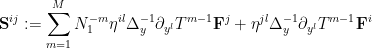
Dear Mr. Tao, , we see from the chain rule that
  is an approximate difference Navier-Stokes-Reynolds flow at U supported on
  , where»
  and so on. I called the slow variables
  , and the fast ones will be
  .
. , and similar relations. So when I compute the Laplacian, abbreviating
  , I should get
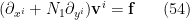
 ![\Delta_{\underline x}v(t,\underline x)=[(\partial_x+N_1\partial_X)^2+(\partial_y+N_1\partial_Y)^2+(\partial_z+N_1\partial_Z)^2]\boldmath v(t,\underline x,\underline X)=[\partial_x^2+2N_1\partial_x\partial_X+N_1^2\partial_X^2+\partial_y^2+2N_1\partial_y\partial_Y+N_1^2\partial_Y^2+\partial_z^2+2N_1\partial_z\partial_Z+N_1^2\partial_Z^2]\boldmath v(t,\underline x,\underline X)=(\Delta_{\underline x}+N_1^2\Delta_{\underline X}+2N_1\nabla_{\underline x}\cdot\nabla_{\underline X}](https://s0.wp.com/latex.php?latex=%5CDelta_%7B%5Cunderline+x%7Dv%28t%2C%5Cunderline+x%29%3D%5B%28%5Cpartial_x%2BN_1%5Cpartial_X%29%5E2%2B%28%5Cpartial_y%2BN_1%5Cpartial_Y%29%5E2%2B%28%5Cpartial_z%2BN_1%5Cpartial_Z%29%5E2%5D%5Cboldmath+v%28t%2C%5Cunderline+x%2C%5Cunderline+X%29%3D%5B%5Cpartial_x%5E2%2B2N_1%5Cpartial_x%5Cpartial_X%2BN_1%5E2%5Cpartial_X%5E2%2B%5Cpartial_y%5E2%2B2N_1%5Cpartial_y%5Cpartial_Y%2BN_1%5E2%5Cpartial_Y%5E2%2B%5Cpartial_z%5E2%2B2N_1%5Cpartial_z%5Cpartial_Z%2BN_1%5E2%5Cpartial_Z%5E2%5D%5Cboldmath+v%28t%2C%5Cunderline+x%2C%5Cunderline+X%29%3D%28%5CDelta_%7B%5Cunderline+x%7D%2BN_1%5E2%5CDelta_%7B%5Cunderline+X%7D%2B2N_1%5Cnabla_%7B%5Cunderline+x%7D%5Ccdot%5Cnabla_%7B%5Cunderline+X%7D&bg=ffffff&fg=545454&s=0&c=20201002) .
. and company.
I have a small question.
In this post, you say «For any shift
From the chain rule,
However, the equations that define approximate fast-slow solutions do not have any trace of those mixed terms. Am I missing something? Can we say those terms are zero? Otherwise what becomes of them?
PS You have an \eqref[bd-5} which does not render because of that open square bracket, it is around the point where you define
[Corrected (and missing terms reinstated), thanks – T.]