246A, Notes 5: conformal mapping

Previous set of notes: Notes 4. Next set of notes: 246B Notes 1.

In the previous set of notes we introduced the notion of a complex diffeomorphism ${f: U \rightarrow V}$ between two open subsets ${U,V}$ of the complex plane ${{\bf C}}$ (or more generally, two Riemann surfaces): an invertible holomorphic map whose inverse was also holomorphic. (Actually, the last part is automatic, thanks to Exercise 41 of Notes 4.) Such maps are also known as biholomorphic maps or conformal maps (although in some literature the notion of “conformal map” is expanded to permit maps such as the complex conjugation map ${z \mapsto \overline{z}}$ that are angle-preserving but not orientation-preserving, as well as maps such as the exponential map ${z \mapsto \exp(z)}$ from ${{\bf C}}$ to ${{\bf C} \backslash \{0\}}$ that are only locally injective rather than globally injective). Such complex diffeomorphisms can be used in complex analysis (or in the analysis of harmonic functions) to change the underlying domain ${U}$ to a domain that may be more convenient for calculations, thanks to the following basic lemma:

Lemma 1 (Holomorphicity and harmonicity are conformal invariants) Let ${\phi: U \rightarrow V}$ be a complex diffeomorphism between two Riemann surfaces ${U,V}$ .

(i) If ${f: V \rightarrow W}$ is a function to another Riemann surface ${W}$ , then ${f}$ is holomorphic if and only if ${f \circ \phi: U \rightarrow W}$ is holomorphic.

(ii) If ${U,V}$ are open subsets of ${{\bf C}}$ and ${u: V \rightarrow {\bf R}}$ is a function, then ${u}$ is harmonic if and only if ${u \circ \phi: U \rightarrow {\bf R}}$ is harmonic.

Proof: Part (i) is immediate since the composition of two holomorphic functions is holomorphic. For part (ii), observe that if ${u: V \rightarrow {\bf R}}$ is harmonic then on any ball ${B(z_0,r)}$ in ${V}$ , ${u}$ is the real part of some holomorphic function ${f: B(z_0,r) \rightarrow {\bf C}}$ thanks to Exercise 62 of Notes 3. By part (i), ${f \circ \phi: \phi^{-1}(B(z_0,r)) \rightarrow {\bf C}}$ is also holomorphic. Taking real parts we see that ${u \circ \phi}$ is harmonic on each ball preimage ${\phi^{-1}(B(z_0,r))}$ in ${V}$ , and hence harmonic on all of ${V}$ , giving one direction of (ii); the other direction is proven similarly. $\Box$

Exercise 2 Establish Lemma 1(ii) by direct calculation, avoiding the use of holomorphic functions. (Hint: the calculations are cleanest if one uses Wirtinger derivatives, as per Exercise 27 of Notes 1.)

Exercise 3 Let ${\phi: U \rightarrow V}$ be a complex diffeomorphism between two open subsets ${U,V}$ of ${{\bf C}}$ , let ${z_0}$ be a point in ${U}$ , let ${m}$ be a natural number, and let ${f: V \rightarrow {\bf C} \cup \{\infty\}}$ be holomorphic. Show that ${f: V \rightarrow {\bf C} \cup \{\infty\}}$ has a zero (resp. a pole) of order ${m}$ at ${\phi(z_0)}$ if and only if ${f \circ \phi: U \rightarrow {\bf C} \cup \{\infty\}}$ has a zero (resp. a pole) of order ${m}$ at ${z_0}$ .

From Lemma 1(ii) we can now define the notion of a harmonic function ${u: M \rightarrow {\bf R}}$ on a Riemann surface ${M}$ ; such a function ${u}$ is harmonic if, for every coordinate chart ${\phi_\alpha: U_\alpha \rightarrow V_\alpha}$ in some atlas, the map ${u \circ \phi_\alpha^{-1}: V_\alpha \rightarrow {\bf R}}$ is harmonic. Lemma 1(ii) ensures that this definition of harmonicity does not depend on the choice of atlas. Similarly, using Exercise 3 one can define what it means for a holomorphic map ${f: M \rightarrow {\bf C} \cup \{\infty\}}$ on a Riemann surface ${M}$ to have a pole or zero of a given order at a point ${p_0 \in M}$ , with the definition being independent of the choice of atlas; we can also identify such functions as equivalence classes of meromorphic functions ${f: M \backslash S \rightarrow {\bf C}}$ in complete analogy with the case of meromorphic functions on domains ${U}$ . Finally, we can define the notion of an essential singularity of a holomorphic function ${f: M \backslash S \rightarrow {\bf C}}$ at some isolated singularity ${p \in S}$ in a Riemann surface as one that cannot be extended to a holomorphic function ${f: (M \backslash S) \cup \{p\} \rightarrow{\bf C} \cup \{\infty\}}$ .

In view of Lemma 1, it is thus natural to ask which Riemann surfaces are complex diffeomorphic to each other, and more generally to understand the space of holomorphic maps from one given Riemann surface to another. We will initially focus attention on three important model Riemann surfaces:

(i) (Elliptic model) The Riemann sphere ${{\bf C} \cup \{\infty\}}$ ;
(ii) (Parabolic model) The complex plane ${{\bf C}}$ ; and
(iii) (Hyperbolic model) The unit disk ${D(0,1)}$ .

The designation of these model Riemann surfaces as elliptic, parabolic, and hyperbolic comes from Riemannian geometry, where it is natural to endow each of these surfaces with a constant curvature Riemannian metric which is positive, zero, or negative in the elliptic, parabolic, and hyperbolic cases respectively. However, we will not discuss Riemannian geometry further here.

All three model Riemann surfaces are simply connected, but none of them are complex diffeomorphic to any other; indeed, there are no non-constant holomorphic maps from the Riemann sphere to the plane or the disk, nor are there any non-constant holomorphic maps from the plane to the disk (although there are plenty of holomorphic maps going in the opposite directions). The complex automorphisms (that is, the complex diffeomorphisms from a surface to itself) of each of the three surfaces can be classified explicitly. The automorphisms of the Riemann sphere turn out to be the Möbius transformations ${z \mapsto \frac{az+b}{cz+d}}$ with ${ad-bc \neq 0}$ , also known as fractional linear transformations. The automorphisms of the complex plane are the linear transformations ${z \mapsto az+b}$ with ${a \neq 0}$ , and the automorphisms of the disk are the fractional linear transformations of the form ${z \mapsto e^{i\theta} \frac{\alpha - z}{1 - \overline{\alpha} z}}$ for ${\theta \in {\bf R}}$ and ${\alpha \in D(0,1)}$ . Holomorphic maps ${f: D(0,1) \rightarrow D(0,1)}$ from the disk ${D(0,1)}$ to itself that fix the origin obey a basic but incredibly important estimate known as the Schwarz lemma: they are “dominated” by the identity function ${z \mapsto z}$ in the sense that ${|f(z)| \leq |z|}$ for all ${z \in D(0,1)}$ . Among other things, this lemma gives guidance to determine when a given Riemann surface is complex diffeomorphic to a disk; we shall discuss this point further below.

It is a beautiful and fundamental fact in complex analysis that these three model Riemann surfaces are in fact an exhaustive list of the simply connected Riemann surfaces, up to complex diffeomorphism. More precisely, we have the Riemann mapping theorem and the uniformisation theorem:

Theorem 4 (Riemann mapping theorem) Let ${U}$ be a simply connected open subset of ${{\bf C}}$ that is not all of ${{\bf C}}$ . Then ${U}$ is complex diffeomorphic to ${D(0,1)}$ .

Theorem 5 (Uniformisation theorem) Let ${M}$ be a simply connected Riemann surface. Then ${M}$ is complex diffeomorphic to ${{\bf C} \cup \{\infty\}}$ , ${{\bf C}}$ , or ${D(0,1)}$ .

As we shall see, every connected Riemann surface can be viewed as the quotient of its simply connected universal cover by a discrete group of automorphisms known as deck transformations. This in principle gives a complete classification of Riemann surfaces up to complex diffeomorphism, although the situation is still somewhat complicated in the hyperbolic case because of the wide variety of discrete groups of automorphisms available in that case.

We will prove the Riemann mapping theorem in these notes, using the elegant argument of Koebe that is based on the Schwarz lemma and Montel’s theorem (Exercise 58 of Notes 4). The uniformisation theorem is however more difficult to establish; we discuss some components of a proof (based on the Perron method of subharmonic functions) here, but stop short of providing a complete proof.

The above theorems show that it is in principle possible to conformally map various domains into model domains such as the unit disk, but the proofs of these theorems do not readily produce explicit conformal maps for this purpose. For some domains we can just write down a suitable such map. For instance:

Exercise 6 (Cayley transform) Let ${{\bf H} := \{ z \in {\bf C}: \mathrm{Im} z > 0 \}}$ be the upper half-plane. Show that the Cayley transform ${\phi: {\bf H} \rightarrow D(0,1)}$ , defined by

$\displaystyle \phi(z) := \frac{z-i}{z+i},$

is a complex diffeomorphism from the upper half-plane ${{\bf H}}$ to the disk ${D(0,1)}$ , with inverse map ${\phi^{-1}: D(0,1) \rightarrow {\bf H}}$ given by

$\displaystyle \phi^{-1}(w) := i \frac{1+w}{1-w}.$

Exercise 7 Show that for any real numbers ${a<b}$ , the strip ${\{ z \in {\bf C}: a < \mathrm{Re}(z) < b \}}$ is complex diffeomorphic to the disk ${D(0,1)}$ . (Hint: use the complex exponential and a linear transformation to map the strip onto the half-plane ${{\bf H}}$ .)

Exercise 8 Show that for any real numbers ${a<b<a+2\pi}$ , the strip ${\{ re^{i\theta}: r>0, a < \theta < b \}}$ is complex diffeomorphic to the disk ${D(0,1)}$ . (Hint: use a branch of either the complex logarithm, or of a complex power ${z \mapsto z^\alpha}$ .)

We will discuss some other explicit conformal maps in this set of notes, such as the Schwarz-Christoffel maps that transform the upper half-plane ${{\bf H}}$ to polygonal regions. Further examples of conformal mapping can be found in the text of Stein-Shakarchi.

— 1. Maps between the model Riemann surfaces —

In this section we study the various holomorphic maps, and conformal maps, between the three model Riemann surfaces ${{\bf C} \cup \{\infty\}}$ , ${{\bf C}}$ , and ${D(0,1)}$ .

From Exercise 20 of Notes 4, we know that the only holomorphic maps ${f: {\bf C} \cup \{\infty\} \rightarrow {\bf C} \cup \{\infty\}}$ from the Riemann sphere to itself (besides the constant function ${\infty}$ ) take the form of a rational function ${f(z) = P(z) / Q(z)}$ away from the zeroes of ${Q}$ (and from ${\infty}$ ), with these singularities all being removable, and with ${Q}$ not identically zero. We can of course reduce to lowest terms and assume that ${P}$ and ${Q}$ have no common factors. In particular, if ${f}$ is to take values in ${{\bf C}}$ rather than ${{\bf C} \cup \{\infty\}}$ , then ${Q}$ can have no roots (since ${f}$ will have a pole at these roots) and so by the fundamental theorem of algebra ${Q}$ is constant and ${f}$ is a polynomial; in order for ${f}$ to have no pole at infinity, ${f}$ must then be constant. Thus the only holomorphic maps from ${{\bf C} \cup \{\infty\}}$ to ${{\bf C}}$ are the constants; in particular, the only holomorphic maps from ${{\bf C} \cup \{\infty\}}$ to ${D(0,1)}$ are the constants. In particular, ${{\bf C} \cup \{\infty\}}$ is not complex diffeomorphic to ${{\bf C}}$ or ${D(0,1)}$ (this is also topologically obvious since the Riemann sphere is compact, and ${{\bf C}}$ and ${D(0,1)}$ are not).

Exercise 9 More generally, show that if ${M}$ is a connected compact Riemann surface and ${N}$ is a connected non-compact Riemann surface, then the only holomorphic maps from ${M}$ to ${N}$ are the constants. (Hint: use the open mapping theorem, Theorem 38 of Notes 4.)

Now we consider complex automorphisms of the Riemann sphere ${{\bf C} \cup \{\infty\}}$ to itself. There are some obvious examples of such automorphisms:

Translation maps ${z \mapsto z + c}$ for some ${c \in {\bf C}}$ , with the convention that ${\infty}$ is mapped to ${\infty}$ ;
Dilation maps ${z \mapsto \lambda z}$ for some ${\lambda \in {\bf C} \backslash \{0\}}$ , with the convention that ${\infty}$ is mapped to ${\infty}$ ; and
The inversion map ${z \mapsto 1/z}$ , with the convention that ${\infty}$ is mapped to ${0}$ .

More generally, given any complex numbers ${a,b,c,d}$ with ${ad-bc \neq 0}$ , we can define the Möbius transformation (or fractional linear transformation) ${z \mapsto \frac{az+b}{cz+d}}$ for ${z \neq \infty, -d/c}$ , with the convention that ${-d/c}$ is mapped to ${\infty}$ and ${\infty}$ is mapped to ${a/c}$ (where we adopt the further convention that ${a/0=\infty}$ for non-zero ${a}$ ). For ${c=0}$ , this is an affine transformation ${z \mapsto \frac{a}{d} z + \frac{b}{d}}$ , which is clearly a composition of a translation and dilation map; for ${c \neq 0}$ , this is a combination ${z \mapsto \frac{a}{c} - \frac{ad-bc}{cz+d}}$ of translations, dilations, and the inversion map. Thus all Möbius transformations are formed from composition of the translations, dilations, and inversions, and in particular are also automorphisms of the Riemann sphere; it is also easy to see that the Möbius transformations are closed under composition, and are thus the group generated by the translations, dilations, and inversions.

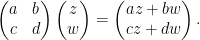
One can interpret the Möbius transformations as projective linear transformations as follows. Recall that the general linear group ${GL_2({\bf C})}$ is the group of ${2 \times 2}$ matrices ${\begin{pmatrix} a & b \\ c & d \end{pmatrix}}$ with non-vanishing determinant ${ad-bc}$ . Clearly every such matrix generates a Möbius transformation ${z \mapsto \frac{az+b}{cz+d}}$ . However, two different elements of ${GL_2({\bf C})}$ can generate the same Möbius transformation if they are scalar multiples of each other. If we define the projective linear group ${PGL_2({\bf C})}$ to be the quotient group of ${GL_2({\bf C})}$ by the group of scalar invertible matrices, then we may identify the set of Möbius transformations with ${PGL_2({\bf C})}$ . The group ${GL_2({\bf C})}$ acts on the space ${{\bf C}^2}$ by the usual map

$\displaystyle \begin{pmatrix} a & b \\ c & d \end{pmatrix} \begin{pmatrix} z \\ w \end{pmatrix} = \begin{pmatrix} az+bw \\ cz+dw \end{pmatrix}.$

If we let ${{\bf CP}^1}$ be the complex projective line, that is to say the space of one-dimensional subspaces of ${{\bf C}^2}$ , then ${GL_2({\bf C})}$ acts on this space also, with the action of the scalars being trivial, so we have an action of ${PGL_2({\bf C})}$ on ${{\bf CP}^1}$ . We can identify the Riemann sphere ${{\bf C} \cup \{\infty\}}$ with the complex projective line by identifying each ${c \in {\bf C} \subset {\bf C} \cup \{\infty\}}$ with the one-dimensional subspace ${\{ (cw,w): w \in {\bf C} \}}$ of ${{\bf C}^2}$ , and identifying ${\infty \in {\bf C} \cup \{\infty\}}$ with ${\{ (z,0): z \in {\bf C}\}}$ . With this identification, one can check that the action of ${PGL_2({\bf C})}$ on ${{\bf CP}^1}$ has become identified with the action of the group of Möbius transformations on ${{\bf C} \cup \{\infty\}}$ . (In particular, the group of Möbius transformations is isomorphic to ${PGL_2({\bf C})}$ .)
There are enough Möbius transformations available that their action on the Riemann sphere is not merely transitive, but is in fact ${3}$ -transitive:

Lemma 10 ( ${3}$ -transitivity) Let ${z_1,z_2,z_3}$ be distinct elements of the Riemann sphere ${{\bf C} \cup \{\infty\}}$ , and let ${w_1,w_2,w_3}$ also be three distinct elements of the Riemann sphere. Then there exists a unique Möbius transformation ${T}$ such that ${T(z_j) = w_j}$ for ${j=1,2,3}$ .

Proof: We first show existence. As the Möbius transformations form a group, it suffices to verify the claim for a single choice of ${z_1,z_2,z_3}$ , for instance ${z_1 = 0, z_2 = 1, z_3 = \infty}$ . If ${w_3=\infty}$ then the affine transformation ${z \mapsto w_1 + z(w_2-w_1)}$ will have the desired properties. If ${w_3 \neq \infty}$ , we can use translation and inversion to find a Möbius transformation ${S}$ that maps ${w_3}$ to ${\infty}$ ; applying the previous case with ${w_1,w_2,w_3}$ with ${S(w_1), S(w_2), S(w_3)}$ and then applying ${S^{-1}}$ , we obtain the claim.

Now we prove uniqueness. By composing on the left and right with Möbius transforms we may assume that ${z_1=w_1=0, z_2=w_2=1, z_3=w_3=\infty}$ . A Möbius transformation ${z \mapsto \frac{az+b}{cz+d}}$ that fixes ${0,1,\infty}$ must obey the constraints ${b=0, a+b=c+d, c=0}$ and so must be the identity, as required. $\Box$

Möbius transformations are not 4-transitive, thanks to the invariant known as the cross-ratio:

Exercise 11 Define the cross-ratio ${[z_1,z_2; z_3,z_4]}$ between four distinct points ${z_1,z_2,z_3,z_4}$ on the Riemann sphere ${{\bf C} \cup \{\infty\}}$ by the formula

$\displaystyle [z_1,z_2; z_3,z_4] = \frac{(z_1-z_3)(z_2-z_4)}{(z_2-z_3)(z_1-z_4)}$

if all of ${z_1,z_2,z_3,z_4}$ avoid ${\infty}$ , and extended continuously to the case when one of the points equals ${\infty}$ (e.g. ${[z_1,z_2;z_3,\infty] = \frac{z_1-z_3}{z_2-z_3}}$ ).

(i) Show that an injective map ${T: {\bf C} \cup \{\infty\} \rightarrow {\bf C} \rightarrow \{\infty\}}$ is a Möbius transform if and only if it preserves the cross-ratio, that is to say that ${[T(z_1),T(z_2);T(z_3),T(z_4)] = [z_1,z_2;z_3,z_4]}$ for all distinct points ${z_1,z_2,z_3,z_4 \in {\bf C} \cup \{\infty\}}$ . (Hint: for the “only if” part, work with the basic Möbius transforms. For the “if” part, reduce to the case when ${T}$ fixes three points, such as ${0,1,\infty}$ .)

(ii) If ${z_1,z_2,z_3,z_4}$ are distinct points in ${{\bf C} \cup \{\infty\}}$ , show that ${z_1,z_2,z_3,z_4}$ lie on a common extended line (i.e., a line in ${{\bf C}}$ together with ${\infty}$ ) or circle in ${{\bf C}}$ if and only if the cross-ratio ${[z_1,z_2;z_3,z_4]}$ is real. Conclude that a Möbius transform will map an extended line or circle to an extended line or circle.

As one quick application of Möbius transformations, we have

Proposition 12 ${{\bf C} \cup \{\infty\}}$ is simply connected.

Proof: We have to show that any closed curve ${\gamma}$ in ${{\bf C} \cup \{\infty\}}$ is contractible to a point in ${{\bf C} \cup \{\infty\}}$ . By deforming ${\gamma}$ locally into line segments in either of the two standard coordinate charts of ${{\bf C} \cup \{\infty\}}$ we may assume that ${\gamma}$ is the concatenation of finitely many such line segments; in particular, ${\gamma}$ cannot be a space-filling curve (as one can see from e.g. the Baire category theorem) and thus avoids at least one point in ${{\bf C} \cup \{\infty\}}$ . If ${\gamma}$ avoids ${\infty}$ then it lies in ${{\bf C}}$ and can thus be contracted to a point in ${{\bf C}}$ (and hence in ${{\bf C} \cup \{\infty\}}$ ) since ${{\bf C}}$ is convex. If ${\gamma}$ avoids any other point ${z_0}$ , then we can apply a Möbius transformation to move ${z_0}$ to ${\infty}$ , contract the transformed curve to a point, and then invert the Möbius transform to contract ${\gamma}$ to a point in ${{\bf C} \cup \{\infty\}}$ . $\Box$

Exercise 13 (Jordan curve theorem in the Riemann sphere) Let ${\gamma: [a,b] \rightarrow {\bf C} \cup \{\infty\}}$ be a simple closed curve in the Riemann sphere. Show that the complement of ${\gamma([a,b])}$ in ${{\bf C} \cup \{\infty\}}$ is the union of two disjoint simply connected open subsets of ${{\bf C} \cup \{\infty\}}$ . (Hint: one first has to exclude the possibility that ${\gamma}$ is space-filling. Do this by verifying that ${\gamma([a,b])}$ is homeomorphic to the unit circle.)

It turns out that there are no other automorphisms of the Riemann sphere than the Möbius transformations:

Proposition 14 (Automorphisms of Riemann sphere) Let ${T: {\bf C} \cup \{\infty\} \rightarrow {\bf C} \cup \{\infty\}}$ be a complex diffeomorphism. Then ${T}$ is a Möbius transformation.

Proof: By Lemma 10 and composing ${T}$ with a Möbius transformation, we may assume without loss of generality that ${T}$ fixes ${0,1,\infty}$ . From Exercise 20 of Notes 4 we know that ${T}$ is a rational function ${T(z) = P(z)/Q(z)}$ (with all singularities removed); we may reduce terms so that ${P,Q}$ have no common factors. Since ${T}$ is bijective and fixes ${\infty}$ , it has no poles in ${{\bf C}}$ , and hence ${Q}$ can have no roots; by the fundamental theorem of algebra, this makes ${Q}$ constant. Similarly, ${P}$ has no zeroes other than ${0}$ , and so must be a monomial; as ${T}$ also fixes ${1}$ , it must be of the form ${T(z) = z^n}$ for some natural number ${n}$ . But this is only injective if ${n=1}$ , in which case ${T}$ is clearly a Möbius transformation. $\Box$

Now we look at holomorphic maps on ${{\bf C}}$ . There are plenty of holomorphic maps from ${{\bf C}}$ to ${{\bf C}}$ ; indeed, these are nothing more than the entire functions, of which there are many (indeed, an entire function is nothing more than a power series with an infinite radius of convergence). There are even more holomorphic maps from ${{\bf C}}$ to ${{\bf C} \cup \{\infty\}}$ , as these are just the meromorphic functions on ${{\bf C}}$ . For instance, any ratio ${f/g}$ of two entire functions, with ${g}$ not identically zero, will be meromorphic on ${{\bf C}}$ . On the other hand, from Liouville’s theorem (Theorem 28 of Notes 3) we see that the only holomorphic maps from ${{\bf C}}$ to ${D(0,1)}$ are the constants. In particular, ${{\bf C}}$ and ${D(0,1)}$ are not complex diffeomorphic (despite the fact that they are diffeomorphic over the reals, as can be seen for instance by using the projection ${z \mapsto \frac{z}{\sqrt{1+|z|^2}}}$ ).

The affine maps ${z \mapsto az+b}$ with ${a \in {\bf C} \backslash \{0\}}$ and ${b \in {\bf C}}$ are clearly complex automorphisms on ${{\bf C}}$ . In analogy with Proposition 14, these turn out to be the only automorphisms:

Proposition 15 (Automorphisms of complex plane) Let ${T: {\bf C} \rightarrow {\bf C}}$ be a complex diffeomorphism. Then ${T}$ is an affine transformation ${T(z) = az+b}$ for some ${a \in {\bf C} \backslash \{0\}}$ and ${b \in {\bf C}}$ .

Proof: By the open mapping theorem (Theorem 38 of Notes 4), ${T(D(0,1))}$ is open, and hence ${T}$ avoids the non-empty open set ${T(D(0,1))}$ on ${{\bf C} \backslash D(0,1)}$ . By the Casorati-Weierstrass theorem (Theorem 12 of Notes 4), we conclude that ${T}$ does not have an essential singularity at infinity. Thus ${T}$ extends to a holomorphic function from ${{\bf C} \cup \{\infty\}}$ to ${{\bf C} \cup \{\infty\}}$ , hence by Exercise 20 of Notes 4 is rational. As the only pole of ${T}$ is at infinity, ${T}$ is a polynomial; as ${T}$ is a diffeomorphism, the derivative has no zeroes and is thus constant by the fundamental theorem of algebra. Thus ${T}$ must be affine, and the claim follows. $\Box$

Exercise 16 Let ${f: {\bf C} \rightarrow {\bf C} \cup \{\infty\}}$ be an injective holomorphic map. Show that ${f}$ is a Möbius transformation (restricted to ${{\bf C}}$ ).

We remark that injective holomorphic maps are often referred to as univalent functions in the literature.

Finally, we consider holomorphic maps on ${D(0,1)}$ . There are plenty of holomorphic maps from ${D(0,1)}$ to ${{\bf C}}$ (indeed, these are just the power series with radius of convergence at least ${1}$ ), and even more holomorphic maps from ${D(0,1)}$ to ${{\bf C} \cup \{\infty\}}$ (for instance, one can take the quotient of two holomorphic functions ${f,g: D(0,1) \rightarrow {\bf C}}$ with ${g}$ non-zero). There are also many holomorphic maps from ${D(0,1)}$ to ${D(0,1)}$ , for instance one can take any bounded holomorphic function ${f: D(0,1) \rightarrow {\bf C}}$ and multiply it by a small constant. However, we have the following fundamental estimate concerning such functions, the Schwarz lemma:

Lemma 17 (Schwarz lemma) Let ${f: D(0,1) \rightarrow D(0,1)}$ be a holomorphic map such that ${f(0)=0}$ . Then we have ${|f(z)| \leq |z|}$ for all ${z \in D(0,1)}$ . In particular, ${|f'(0)| \leq 1}$ .
Furthermore, if ${|f(z)|=|z|}$ for some ${z \in D(0,1) \backslash \{0\}}$ , or if ${|f'(0)|=1}$ , then there exists a real number ${\theta}$ such that ${f(z) = e^{i \theta} z}$ for all ${z \in D(0,1)}$ .

Proof: By the factor theorem (Corollary 22 of Notes 3), we may write ${f(z) = z g(z)}$ for some holomorphic ${g: D(0,1) \rightarrow {\bf C}}$ . On any circle ${\{ z: |z| = 1-\varepsilon \}}$ with ${0 < \varepsilon < 1}$ , we have ${|f(z)| <1}$ and hence ${|g(z)| < \frac{1}{1-\varepsilon}}$ ; by the maximum principle we conclude that ${|g(z)| \leq \frac{1}{1-\varepsilon}}$ for all ${z \in D(0,1-\varepsilon)}$ . Sending ${\varepsilon}$ to zero, we conclude that ${|g(z)| \leq 1}$ for all ${z \in D(0,1)}$ , and hence ${|f(z)| \leq |z|}$ and ${|f'(0)| \leq 1}$ .

Finally, if ${|f(z)|=|z|}$ for some ${z \in D(0,1) \backslash \{0\}}$ or ${|f'(0)|=1}$ , then ${|g(z)|}$ equals ${1}$ for some ${z \in D(0,1)}$ , and hence by a variant of the maximum principle (see Exercise 18 below) we see that ${g}$ is constant, giving the claim. $\Box$

Exercise 18 (Variant of maximum principle) Let ${U}$ be a connected Riemann surface, and let ${z_0}$ be a point in ${U}$ .

(i) If ${u: U \rightarrow {\bf R}}$ is a harmonic function such that ${u(z) \leq u(z_0)}$ for all ${z \in U}$ , then ${u(z) = u(z_0)}$ for all ${z \in U}$ .

(ii) If ${f: U \rightarrow {\bf C}}$ is a holomorphic function such that ${|f(z)| \leq |f(z_0)|}$ for all ${z \in U}$ , then ${f(z) = f(z_0)}$ for all ${z \in U}$ .

(Hint: use Exercise 17 of Notes 3 .)

One can think of the Schwarz lemma as follows. Let ${{\mathcal H}_0}$ denote the collection of holomorphic functions ${f: D(0,1) \rightarrow D(0,1)}$ with ${f(0)=0}$ . Inside this collection we have the rotations ${R_\theta: D(0,1) \rightarrow D(0,1)}$ for ${\theta \in {\bf R}}$ defined by ${R_\theta(z) :=e^{i\theta} z}$ . The Schwarz lemma asserts that these rotations “dominate” the remaining functions ${f}$ in ${{\mathcal H}_0}$ in the sense that ${|f(z)| \leq |R_\theta(z)|}$ on ${D(0,1) \backslash \{0\}}$ , and in particular ${|f'(z)| \leq |R'_\theta(z)|}$ ; furthermore these inequalities are strict as long as ${f}$ is not one of the ${R_\theta}$ .

As a first application of the Schwarz lemma, we characterise the automorphisms of the disk ${D(0,1)}$ . For any ${\alpha \in D(0,1)}$ , one can check that the Möbius transformation ${z \mapsto \frac{z-\alpha}{1-\overline{\alpha} z}}$ preserves the boundary of the disk ${D(0,1)}$ (since ${1 - \overline{\alpha} z = z \overline{(z-\alpha)}}$ when ${|z|=1}$ ), and maps the point ${\alpha}$ to the origin, and thus maps the disk ${D(0,1)}$ to itself. More generally, for any ${\alpha \in D(0,1)}$ and ${\theta \in {\bf R}}$ , the Möbius transformation ${z \mapsto e^{i\theta} \frac{z-\alpha}{1-\overline{\alpha} z}}$ is an automorphism of the disk ${D(0,1)}$ . It turns out that these are the only such automorphisms:

Theorem 19 (Automorphisms of disk) Let ${f: D(0,1) \rightarrow D(0,1)}$ be a complex diffeomorphism. Then there exists ${\alpha \in D(0,1)}$ and ${\theta \in {\bf R}}$ such that ${f(z) = e^{i\theta} \frac{z-\alpha}{1-\overline{\alpha} z}}$ for all ${z \in D(0,1)}$ . If furthermore ${f(0)=0}$ , then we can take ${\alpha=0}$ , thus ${f(z) =e^{i\theta} z}$ for ${z \in D(0,1)}$ .

Proof: First suppose that ${f(0)=0}$ . By the Schwarz lemma applied to both ${f}$ and its inverse ${f^{-1}}$ , we see that ${|f'(0)|, |(f^{-1})'(0)| \leq 1}$ . But by the inverse function theorem (or the chain rule), ${(f^{-1})'(0) = 1/f'(0)}$ , hence ${|f'(0)|=1}$ . Applying the Schwarz lemma again, we conclude that ${f(z) = e^{i\theta} z}$ for some ${\theta}$ , as required.

In the general case, there exists ${\alpha \in D(0,1)}$ such that ${f(\alpha) = 0}$ . If one then applies the previous analysis to ${f \circ g^{-1}}$ , where ${g: D(0,1) \rightarrow D(0,1)}$ is the automorphism ${g(z) := \frac{z-\alpha}{1-\overline{\alpha} z}}$ , we obtain the claim. $\Box$

Exercise 20 (Automorphisms of half-plane) Let ${f: {\bf H} \rightarrow {\bf H}}$ be a complex diffeomorphism from the upper half-plane ${{\bf H} := \{z \in {\bf C}: \mathrm{Im}(z) > 0 \}}$ to itself. Show that there exist real numbers ${a,b,c,d}$ with ${ad-bc = 1}$ such that ${f(z) = \frac{az+b}{cz+d}}$ for ${z \in {\bf H}}$ . Conclude that the automorphism group of either ${D(0,1)}$ or ${{\bf H}}$ is isomorphic as a group to the projective special linear group ${PSL_2({\bf R})}$ formed by starting with the special linear group ${SL_2({\bf R})}$ of ${2 \times 2}$ real matrices ${\begin{pmatrix} a & b \\ c & d \end{pmatrix}}$ of determinant ${1}$ , and then quotienting out by the central subgroup ${\{ \begin{pmatrix} 1 & 0 \\ 0 & 1 \end{pmatrix}, \begin{pmatrix} -1 & 0 \\ 0 & -1 \end{pmatrix} \}}$ .

Remark 21 Collecting the various assertions above about the holomorphic maps between the elliptic, parabolic, and hyperbolic model Riemann surfaces ${{\bf C} \cup \{\infty\}}$ , ${{\bf C}}$ , ${D(0,1)}$ , one arrives at the following rule of thumb: there are “many” holomorphic maps from “more hyperbolic” surfaces to “less hyperbolic” surfaces, but “very few” maps going in the other direction (and also relatively few automorphisms from one space to an “equally hyperbolic” surface). This rule of thumb also turns out to be accurate in the context of compact Riemann surfaces, where “higher genus” becomes the analogue of “more hyperbolic” (and similarly for “less hyperbolic” or “equally hyperbolic”). One can formalise this latter version of the rule of thumb using such results as the Riemann-Hurwitz formula and the de Franchis theorem, but these are beyond the scope of this course.

Exercise 22 Let ${f: M \rightarrow N}$ be a non-constant holomorphic map between Riemann surfaces ${M,N}$ . If ${M}$ is compact connected and ${N}$ is connected, show that ${f}$ is surjective and ${N}$ is compact. Conclude in particular that there are no non-constant bounded holomorphic functions ${f: M \rightarrow {\bf C}}$ on a compact connected Riemann surface.

— 2. Quotients of the model Riemann surfaces —

The three model Riemann surfaces ${{\bf C} \cup \{\infty\}}$ , ${{\bf C}}$ , ${D(0,1)}$ are all simply connected, and the uniformisation theorem will tell us that up to complex diffeomorphism, these are the only simply connected Riemann surfaces that exist. However, it is possible to form non-simply-connected Riemann surfaces from these model surfaces by the procedure of taking quotients, as follows. Let ${M}$ be a Riemann surface, and let ${\Gamma}$ be a group of complex automorphisms of ${M}$ . We assume that the action of ${\Gamma}$ on ${M}$ is free, which means that the non-identity transformations ${T: M \rightarrow M}$ in ${\Gamma}$ have no fixed points (thus ${T p \neq p}$ for all ${p \in M}$ ). We also assume that the action is proper (viewing ${\Gamma}$ as a discrete group), which means that for any compact subset ${K}$ of ${M}$ , there are only finitely many automorphisms ${T}$ in ${\Gamma}$ for which ${TK}$ intersects ${K}$ . If the action is both free and proper, then we see that every point ${p \in M}$ has a small neighbourhood ${U_p}$ with the property that the images ${TU_p, T \in \Gamma}$ are all disjoint; by making ${U_p}$ small enough we can also find a holomorphic coordinate chart ${\phi_p: U_p \rightarrow V_p}$ to some open subset ${V_p}$ of ${{\bf C}}$ . We can then form the quotient manifold ${\Gamma \backslash M}$ of orbits ${\Gamma p := \{ Tp: T \in \Gamma\}}$ , using the coordinate charts ${\tilde \phi_p: \Gamma \backslash \bigcup_{T \in \Gamma} TU_p \rightarrow V_p}$ for any ${p \in M}$ defined by setting

$\displaystyle \tilde \phi_p( \Gamma q ) := \phi_p( q )$

for all ${q \in U_p}$ . One can easily verify that ${\Gamma \backslash M}$ is a Riemann surface, and that the quotient map ${\pi: M \rightarrow \Gamma \backslash M}$ defined by ${\pi(p) := \Gamma p}$ is a surjective holomorphic covering map. The ability to easily take quotients is one of the key advantages of the Riemann surface formalism; another is the converse ability to construct covers, such as the universal cover of a Riemann surface, defined in Theorem 25 below.

Exercise 23 Let ${M}$ be a Riemann surface, ${\Gamma}$ a group of complex automorphisms of ${M}$ acting in a proper and free fashion, and let ${\pi: M \rightarrow \Gamma \backslash M}$ be the quotient map. Let ${f: M \rightarrow N}$ be a holomorphic map to another Riemann surface ${N}$ . Show that there exists a holomorphic map ${\tilde f: \Gamma \backslash M \rightarrow N}$ such that ${f = \tilde f \circ \pi}$ if and only if ${f = f \circ T}$ for all ${T \in \Gamma}$ .

Remark 24 It is also of interest to quotient a Riemann surface ${M}$ by a group ${\Gamma}$ of complex automorphisms whose action is not free. In that case, the quotient space ${\Gamma \backslash M}$ need not be a manifold, but is instead a more general object known as an orbifold. A typical example is the modular curve ${SL_2({\bf Z}) \backslash {\bf H}}$ (where ${SL_2({\bf Z})}$ is the group of ${2 \times 2}$ matrices with integer coefficients and determinant ${1}$ ); this is of great importance in analytic number theory. However, we will not study orbifolds in this course.

Since the continuous image of a connected space is always connected, we see that any quotient ${\Gamma \backslash M}$ of a connected Riemann surface is again connected. In the converse direction, one can use this construction to describe a connected Riemann surface as a quotient of a simply connected Riemann surface:

Theorem 25 (Universal cover) Let ${M}$ be a connected Riemann surface. Then there exists a simply connected Riemann surface ${N}$ , and a group ${\Gamma}$ of complex automorphisms acting on ${N}$ in a proper and free fashion, such that ${M}$ is complex diffeomorphic to ${\Gamma \backslash N}$ .

Proof: For sake of brevity we omit some of the details of the construction as exercises.

We use the following abstract construction to build the Riemann surface ${N}$ . Fix a base point ${p_0}$ in ${M}$ . For any point ${p}$ in ${M}$ , we can form the space of all continuous paths ${\gamma: [a,b] \rightarrow M}$ from ${p_0}$ to ${p}$ for some interval ${[a,b]}$ with ${a<b}$ . We let ${N_p}$ denote the space of equivalence classes of such paths with respect to the operation of homotopy with fixed endpoints up to reparameterisation; for instance, if ${M}$ was simply connected, then ${N_p}$ would simply be a point. (One could also omit the reparameterisation by restricting the domain of ${\gamma}$ to be a fixed interval such as ${[0,1]}$ .) As ${M}$ is connected, all the ${N_p}$ are non-empty. We then let ${N}$ be the (disjoint) union of all the ${N_p}$ . This defines a set ${N}$ together with a projection map ${\pi: N \rightarrow M}$ that sends all the homotopy classes in ${N_p}$ to ${p}$ for each ${p \in M}$ ; this is clearly a surjective map.

This defines ${N}$ as a set, but we want to give ${N}$ the structure of a Riemann surface, and thus must create an atlas of coordinate charts. For every ${p \in M}$ , let ${\phi_p: U_p \rightarrow D(0,1)}$ be a coordinate chart that is a diffeomorphism between some neighbourhood ${U_p}$ of ${p}$ and the unit disk. Given a homotopy class ${\tilde p}$ in ${N_p}$ and a point ${p'}$ in ${U_p}$ , we can then associate a point ${\tilde p'}$ in ${N_{p'}}$ by taking a path ${\gamma}$ from ${p_0}$ to ${p}$ in the homotopy class ${\tilde p}$ , and concatenating it with the path ${\phi_p^{-1} \circ \gamma_{0 \rightarrow \phi_p(p')}}$ that connects ${p}$ to ${p'}$ via a line segment in the disk ${D(0,1)}$ using the coordinate chart ${\phi_p}$ ; the homotopy class of this concatenated path does not depend on the precise choice of ${\gamma}$ and will be denoted ${\tilde p'}$ . If we let ${\tilde U_{\tilde p}}$ denote all the points ${\tilde p'}$ obtained in this fashion as ${p'}$ varies over ${U_p}$ , then it is easy to see (Exercise!) that the ${\tilde U_{\tilde p}, \tilde p \in N_p}$ are disjoint and partition the set ${\pi^{-1}(U_p)}$ . We can then form coordinate charts ${\tilde \phi_{\tilde p}: \tilde U_{\tilde p} \rightarrow D(0,1)}$ for each ${\tilde p \in N_p}$ and ${p \in M}$ by setting ${\tilde \phi_{\tilde p}(\tilde p') = \phi_p \circ \pi(\tilde p')}$ for all ${\tilde p' \in \tilde U_{\tilde p}}$ . This defines both a topology on ${N}$ (by declaring a subset ${U}$ of ${N}$ to be open if ${\tilde \phi_{\tilde p}( U \cap \tilde U_{\tilde p})}$ is open for all ${\tilde p \in N}$ ) and a complex structure, as the transition maps are easily verified (Exercise!) to be both continuous and holomorphic (after first shrinking the neighbourhoods ${U_p}$ and ${\tilde U_p}$ if necessary). By construction we now see that ${N}$ is a covering space of ${M}$ , with ${\pi: N \rightarrow M}$ the covering map.

Let ${\tilde p_0 \in N_{p_0}}$ be the homotopy class of the constant curve at ${p_0}$ . It is easy to see (Exercise!) that ${N}$ is connected (indeed, any point ${\tilde p}$ in ${N}$ determines (more or less tautologically) a family of paths in ${N}$ from ${\tilde p_0}$ to ${\tilde p}$ ). Next, we make the stronger claim that ${N}$ is simply connected. It suffices to show that any closed path ${\tilde \gamma: [0,1] \rightarrow N}$ from ${\tilde p_0}$ to ${\tilde p_0}$ is contractible to a point. Let ${\gamma: [0,1] \rightarrow M}$ denote the projected curve ${\gamma := \pi \circ \tilde \gamma}$ , thus ${\gamma}$ is a closed curve from ${p_0}$ to itself. From the continuity method (Exercise!) we see that for any ${0 \leq t \leq 1}$ , the restriction ${\gamma_{[0,t]}: [0,t] \rightarrow M}$ of ${\gamma}$ to ${[0,t]}$ lies in the homotopy class of ${\tilde \gamma(t)}$ ; in particular, ${\gamma}$ itself lies in the homotopy class of ${\tilde p_0}$ , and is thus homotopic to a point. Another application of the continuity method (Exercise!) then shows that as one continuously deforms ${\gamma}$ to a point, each of the curves ${\gamma_s}$ obtained in this deformation lifts to a closed curve ${\tilde \gamma_s}$ in ${N}$ from ${\tilde p_0}$ to ${\tilde p_0}$ , in the sense that ${\gamma_s = \pi \circ \tilde \gamma_s}$ ; furthermore, ${\tilde \gamma_s}$ varies continuously in ${s}$ , giving the required homotopy from ${\tilde \gamma}$ to a point.

Define a deck transformation to be a holomorphic map ${T: N \rightarrow N}$ such that ${\pi \circ T = \pi}$ (that is to say, ${T}$ preserves each of the “fibres” ${N_p}$ of ${N}$ ). Clearly the composition of two deck transformations is again a deck transformation. From Corollary 51 of Notes 4 we see that for any ${p \in M}$ and ${\tilde p, \tilde q \in N_p}$ , there exists a unique deck transformations that maps ${\tilde p}$ to ${\tilde q}$ . Composing that a deck transformations with the deck transformations that maps ${\tilde q}$ to ${\tilde p}$ we see that all deck transformations are invertible and are thus complex automorphisms. If we let ${\Gamma}$ denote the collection of all deck transformations then we see that ${\Gamma}$ is a group that acts freely on ${N}$ and transitively on each fibre ${N_p}$ . For any ${p \in M}$ , and the neighbourhoods ${U_p}$ as before, one can verify (Exercise!) that each deck transformation in ${\Gamma}$ permutes the disjoint open sets ${\tilde U_{\tilde p}, \tilde p \in N_p}$ covering ${U_p}$ , and given any two of these sets ${\tilde U_{\tilde p}, \tilde U_{\tilde q}}$ there is exactly one deck transformation that maps ${\tilde U_{\tilde p}}$ to ${\tilde U_{\tilde q}}$ . From this one can check (Exercise!) that ${\Gamma \backslash N}$ is complex diffeomorphic to ${M}$ as required. $\Box$

Exercise 26 Write out the steps marked “Exercise!” in the above argument.

The manifold ${N}$ in the above theorem is called a universal cover of ${M}$ , and the group ${\Gamma}$ is (a copy of) the fundamental group of ${M}$ . These objects are basically uniquely determined by ${M}$ :

Exercise 27 Suppose one has two simply connected Riemann surfaces ${N, N'}$ and two groups ${\Gamma, \Gamma'}$ of automorphisms of ${N, N'}$ respectively acting in proper and free fashions. Show that the following statements are equivalent:

(i) The quotients ${\Gamma \backslash N}$ and ${\Gamma' \backslash N'}$ are complex diffeomorphic.

(ii) There exists a complex diffeomorphism ${\phi: N \rightarrow N'}$ and a group isomorphism ${\iota: \Gamma \rightarrow \Gamma'}$ such that
$\displaystyle \iota(T) (\phi(p)) = \phi( Tp ) \ \ \ \ \ (1)$

for all ${p \in N}$ and ${T \in \Gamma}$ . In particular ${N}$ and ${N'}$ are complex diffeomorphic, and the groups ${\Gamma}$ and ${\Gamma'}$ are isomorphic.

(Hint: use Exercise 23 for one direction of the implication, and Corollary 51 of Notes 4 for the other implication.)

Exercise 28 Let ${M}$ be a connected Riemann surface, and let ${p_0}$ be a point in ${M}$ . Define the fundamental group ${\pi_1(M)}$ based at ${p_0}$ to be the collection of equivalence classes ${[\gamma]}$ of closed curves ${\gamma:[a,b] \rightarrow M}$ from ${p_0}$ to ${p_0}$ , under the relation of homotopy with fixed endpoints up to reparameterisation.

(i) Show that ${\pi_1(M)}$ is indeed a group, with the equivalence class of the constant curves as the identity element, the inverse of a homotopy class ${[\gamma]}$ of a curve ${\gamma}$ defined as ${[-\gamma]}$ , and the product ${[\gamma_1] [\gamma_2]}$ of two homotopy classes of curves ${\gamma_1,\gamma_2}$ as ${[\gamma_1+\gamma_2]}$ .

(ii) If ${N, \Gamma}$ are as in Theorem 25, show that ${\Gamma}$ is isomorphic to ${\pi_1(M)}$ .

Exercise 29 Show that the fundamental group of ${{\bf C} \backslash \{0\}}$ is isomorphic to the integers ${{\bf Z}}$ (viewed as an additive group).

Exercise 30 (Universality) Let ${M}$ be a connected Riemann surface, let ${N}$ be a universal cover of ${M}$ with covering map ${\pi: N \rightarrow M}$ , and let ${L}$ be another Riemann surface cover of ${M}$ with a covering map ${\psi: L \rightarrow M}$ . Let ${p_0}$ be a point in ${M}$ , let ${q_0 \in N}$ be a point in ${\pi^{-1}(p_0)}$ , and let ${r_0}$ be a point in ${\psi^{-1}(r_0)}$ . Show that there is a unique covering map ${\phi: N \rightarrow L}$ with ${\phi(q_0)=r_0}$ such that ${\pi = \psi \circ \phi}$ . This helps justify the terminology “universal cover”.

If we assume for now the uniformisation theorem, we conclude that every connected Riemann surface is the quotient of one of the three model surfaces ${{\bf C} \cup \{\infty\}}$ , ${{\bf C}}$ , ${D(0,1)}$ by a group of complex automorphisms that act freely and properly; depending on which surface is used, we call these Riemann surfaces of elliptic type, parabolic type, and hyperbolic type respectively. We can then study each of the three model types in turn:

Elliptic type: By Proposition 14, the automorphisms of ${{\bf C} \cup \{\infty\}}$ are the Möbius transformations. From the quadratic formula (or the fundamental theorem of algebra) we see that every Möbius transformation has at least one fixed point (for instance, the translations ${z \mapsto z+c}$ fix ${\infty}$ ). Thus the only group of complex automorphisms that can act freely on ${{\bf C} \cup \{\infty\}}$ is the trivial group, so the only Riemann surfaces of elliptic type are those that are complex diffeomorphic to the Riemann sphere.

Parabolic type: By Proposition 14, the automorphisms of ${{\bf C}}$ are the affine transformations ${z \mapsto az+b}$ . These transformations have fixed points in ${{\bf C}}$ if ${a \neq 1}$ , so in order to obtain a free action we must restrict ${\Gamma}$ to the translations ${z \mapsto z+b}$ . Thus we can view ${\Gamma}$ as an additive subgroup of ${{\bf C}}$ , with ${\Gamma \backslash {\bf C}}$ now being the group quotient; as the action is additive, we can also write ${\Gamma \backslash {\bf C}}$ as ${{\bf C} / \Gamma}$ . In order for the action to be proper, ${\Gamma}$ must be a discrete subgroup of ${{\bf C}}$ (every point isolated). We can classify all such subgroups:

Exercise 31 Let ${\Gamma}$ be a discrete additive subgroup of ${{\bf C}}$ . Show that ${\Gamma}$ takes on one of the following three forms:

(i) (Rank zero case) the trivial group ${\{0\}}$ ;

(ii) (Rank one case) a cyclic group ${\omega {\bf Z} := \{ n \omega: n \in {\bf Z}\}}$ for some ${\omega \in {\bf C} \backslash \{0\}}$ ; or

(iii) (Rank two case) a group ${\omega_1 {\bf Z} + \omega_2 {\bf Z} := \{ n_1 \omega_1 + n_2 \omega_2: n_1,n_2 \in {\bf Z} \}}$ for some ${\omega_1,\omega_2 \in {\bf C} \backslash \{0\}}$ with ${\omega_2/\omega_1}$ strictly complex (i.e., not real).

We conclude that every Riemann surface of parabolic type is complex diffeomorphic to a plane ${{\bf C}}$ , a cylinder ${\omega{\bf Z} \backslash {\bf C}}$ for some ${\omega \in {\bf C} \backslash \{0\}}$ , or a torus ${(\omega_1 {\bf Z} + \omega_2{\bf Z}) \backslash {\bf C}}$ for ${\omega_1,\omega_2 \in {\bf C} \backslash \{0\}}$ and ${\omega_1/\omega_2}$ strictly complex.

The case of the plane is self-explanatory. Using dilation maps we see that all cylinders are complex diffeomorphic to each other; for instance, they are all diffeomorphic to ${2\pi i {\bf Z} \backslash {\bf C}}$ . The exponential map ${z \mapsto \exp(z)}$ is ${2\pi i}$ -periodic and thus descends to a map from ${2\pi i {\bf Z} \backslash {\bf C}}$ to ${{\bf C} \backslash \{0\}}$ ; it is easy to see that this map is a complex diffeomorphism, thus the punctured plane ${{\bf C} \backslash \{0\}}$ can be used as a model for all Riemann surface cylinders.

The case of the tori ${(\omega_1 {\bf Z} + \omega_2{\bf Z}) \backslash {\bf C}}$ are more interesting. One can use dilations to normalise one of the ${\omega_1,\omega_2}$ to be a specific value such as ${1}$ , but one cannot normalise both:

Exercise 32 Let ${(\omega_1 {\bf Z} + \omega_2{\bf Z}) \backslash {\bf C}}$ and ${(\omega'_1 {\bf Z} + \omega'_2{\bf Z}) \backslash {\bf C}}$ be two tori. Show that these two tori are complex diffeomorphic if and only if there exists an element ${\begin{pmatrix} a & b \\ c & d \end{pmatrix}}$ of the special linear group ${SL_2({\bf Z})}$ (thus ${a,b,c,d}$ are integers with ${ad-bc=1}$ ) such that

$\displaystyle \frac{\omega'_1}{\omega'_2} = \pm \frac{a \omega_1 + b \omega_2}{c \omega_1 + d \omega_2}.$

(Hint: lift any such diffeomorphism to a holomorphic map from ${{\bf C}}$ to ${{\bf C}}$ of linear growth.)

In contrast to the cylinders ${\omega {\bf Z} \backslash {\bf C}}$ , which are complex diffeomorphic to a subset ${{\bf C} \backslash \{0\}}$ of the complex plane, one cannot model a torus by a subset ${U}$ of ${{\bf C}}$ ; indeed, if there were a complex diffeomorphism ${\phi: (\omega_1 {\bf Z} + \omega_2{\bf Z}) \backslash {\bf C} \rightarrow U}$ , then ${U}$ would have to be non-empty, compact, and (by the open mapping theorem) open in ${{\bf C}}$ , which is impossible since ${{\bf C}}$ is non-compact and connected. However, it is an important fact in algebraic geometry, classical analysis and number theory that these tori can be modeled instead by elliptic curves. The theory of elliptic curves is extremely rich, but is beyond the scope of this course and will not be discussed further here (but the Weierstrass elliptic functions used to construct the complex diffeomorphism between tori and elliptic curves may be covered in subsequent quarters).

Exercise 33 Let ${U}$ be a connected subset of ${{\bf C}}$ that omits at least two points of ${{\bf C}}$ . Show that ${U}$ cannot be of elliptic or parabolic type. (Hint: in addition to the open mapping theorem argument given above, one can use either the little Picard theorem, Theorem 56 of Notes 4, or the simpler Casorati-Weierstrass theorem (Theorem 12 of Notes 4).) In particular, assuming the uniformisation theorem, such sets ${U}$ must be of hyperbolic type. (Note this is compatible with our previous intuition that “more hyperbolic” is analogous to “higher genus” or “has more holes”.)

Hyperbolic type: Here it is convenient to model the hyperbolic Riemann surface using the upper half-plane ${{\bf H}}$ (the Poincaré half-plane model) rather than the disk ${D(0,1)}$ (the Poincaré disk model). By Exercise 20, a Riemann surface of hyperbolic type is then isomorphic to a quotient ${\Gamma \backslash {\bf H}}$ of ${{\bf H}}$ by some subgroup ${\Gamma}$ of ${PSL_2({\bf R})}$ that acts freely and properly. Properness is easily seen to be equivalent to ${\Gamma}$ being a discrete subgroup of ${PSL_2({\bf R})}$ (using the topology inherited from the embedding of ${SL_2({\bf R})}$ in ${{\bf R}^4}$ ); such groups are known as Fuchsian groups. Freeness can also be described explicitly:

Exercise 34 Show that a subgroup ${\Gamma}$ of ${PSL_2({\bf R})}$ acts freely on ${{\bf H}}$ if and only if it avoids all (equivalence classes) of matrices ${\begin{pmatrix} a & b \\ c & d \end{pmatrix}}$ in ${PSL_2({\bf R})}$ that are elliptic in the sense that they obey the trace condition ${|a+d| < 2}$ .

It turns out that in contrast to the elliptic type and parabolic type situations, there are a very large number of possible subgroups ${\Gamma}$ obeying these conditions, and a complete classification of them is basically hopeless. The theory of Fuchsian groups is again very rich, being a foundational topic in hyperbolic geometry, but is again beyond the scope of this course.

Remark 35 The twice-punctured plane ${{\bf C} \backslash \{0,1\}}$ must be of hyperbolic type by the uniformisation theorem and Exercise 33. This gives another proof of the little Picard theorem: an entire function ${f: {\bf C} \rightarrow {\bf C} \backslash \{0,1\}}$ that omits (say) the points ${0,1}$ must then lift (by Corollary 51 of Notes 4) to a holomorphic map from ${{\bf C}}$ to ${D(0,1)}$ , which must then be constant by Liouville’s theorem. A more complicated argument along these lines also proves the great Picard theorem. It turns out that the covering map from ${D(0,1)}$ to ${{\bf C} \backslash \{0,1\}}$ can be described explicitly using the theory of elliptic functions (and specifically the modular lambda function), but this is beyond the scope of this course.

Exercise 36 Show that any annulus ${\{ z: r < |z| < R \}}$ is of hyperbolic type, and is in fact complex diffeomorphic to ${\Gamma \backslash {\bf H}}$ for some cyclic group ${\Gamma}$ of dilations. (Hint: first use the complex exponential to cover the annulus by a strip, then use Exercise 7.)

Exercise 37 (Schottky’s theorem on conformal maps between annuli) Let ${A_1 := \{ z: r_1 < |z| < R_1\}}$ and ${A_2 := \{ z: r_2 < |z| < R_2 \}}$ be two annuli with ${0 < r_1 < R_1}$ and ${0 < r_2 < R_2}$ . Show that ${A_1}$ and ${A_2}$ are complex diffeomorphic if and only if ${R_2/r_2 = R_1/r_1}$ . (Hint: one can either argue by lifting to the half-plane using the previous exercise, or else using the Schwarz reflection principle (adapted to circles in place of lines) repeatedly to extend a holomorphic map from ${A_1}$ to ${A_2}$ to a holomorphic map from a punctured disk to a punctured disk; one can also combine the methods by taking logarithms to lift ${A_1}$ , ${A_2}$ to strips, and then using the original Schwarz reflection principle. This result is due to Schottky, but should not be confused with another theorem of Schottky in complex analysis.)

Exercise 38

(i) Show that the punctured disk ${D(0,1) \backslash \{0\}}$ is of hyperbolic type, and is complex diffeomorphic to ${{\bf Z} \backslash {\bf H}}$ , where ${{\bf Z}}$ acts on ${{\bf H}}$ by translations.

(ii) Show that the Jowkowsky transform ${z \mapsto \frac{1}{2} (z + \frac{1}{z})}$ is a complex diffeomorphism from ${D(0,1)}$ to the slitted extended complex plane ${({\bf C} \cup \{\infty\}) \backslash [-1,1]}$ . Conclude that ${{\bf C} \backslash [-1,1]}$ is also complex diffeomorphic to ${{\bf Z} \backslash {\bf H}}$ .

— 3. The Riemann mapping theorem —

We are now ready to prove the Riemann mapping theorem, Theorem 4, using an argument of Koebe. To motivate the argument, let us rephrase the Schwarz lemma in the following form:

Lemma 39 (Schwarz lemma, again) Let ${U}$ be a Riemann surface, and let ${p_0}$ be a point in ${U}$ . Let ${{\mathcal H}_{p_0}}$ denote the collection of holomorphic functions ${f: U \rightarrow D(0,1)}$ with ${f(p_0) = 0}$ . If ${{\mathcal H}_{p_0}}$ contains an element ${\phi}$ that is a complex diffeomorphism, then ${|f(p)| \leq |\phi(p)|}$ for all ${p \in U \backslash \{p_0\}}$ ; if ${U}$ is a subset of the complex plane ${{\bf C}}$ , we also have ${|f'(p_0)| \leq |\phi'(p_0)|}$ . Furthermore, in either of these two inequalities, equality holds if and only if ${f = e^{i\theta} \phi}$ for some real number ${\theta}$ .

Proof: Apply Lemma 17 to the map ${f \circ \phi^{-1}: D(0,1) \rightarrow D(0,1)}$ . $\Box$

This lemma suggests the following strategy to prove the Riemann mapping theorem: starting with the open subset ${U}$ of the complex plane ${{\bf C}}$ , pick a point ${p_0}$ in that subset, and form the collection ${{\mathcal H}_{p_0}}$ of holomorphic maps ${f: U \rightarrow D(0,1)}$ that map ${p_0}$ to ${0}$ , and locate an element ${\phi}$ of this collection for which the magnitude ${|\phi'(p_0)|}$ is maximal. If the Riemann mapping theorem were true, then Lemma 39 would ensure that this ${\phi}$ would be a complex diffeomorphism, and we would be done.

It turns out to be convenient to work with the somewhat smaller collection ${{\mathcal I}_{p_0}}$ of injective holomorphic maps ${f: U \rightarrow D(0,1)}$ (also known as univalent functions from ${U}$ to ${D(0,1)}$ ). We first observe that this collection is non-empty for the sets ${U}$ of interest:

Proposition 40 Let ${U}$ be a simply connected subset of ${{\bf C}}$ that is not all of ${{\bf C}}$ . Then there exists an injective holomorphic map ${f: U \rightarrow D(0,1)}$ .

Proof: By applying a translation to ${U}$ , we may assume that ${U}$ avoids the origin ${0}$ . If ${U}$ in fact avoided a disk ${D(z_0,r)}$ , then we could use the map ${z \mapsto \frac{r}{2(z-z_0)}}$ to map ${U}$ injectively into the disk ${D(0,1)}$ . At present, ${U}$ need not avoid any disk (e.g. ${U}$ could be the complex plane with the negative axis ${\{ t \in {\bf R}: t \leq 0 \}}$ removed). However, as ${U}$ is simply connected and avoids ${0}$ , we can argue as in Section 4 of Notes 4 to obtain a holomorphic branch ${f: U \rightarrow {\bf C} \backslash \{0\}}$ of the square root function, that is to say a holomorphic map ${f}$ such that ${f^2(z) = z}$ for all ${z \in U}$ . As ${f^2}$ is injective, ${f}$ must also be injective; it is also clearly non-constant, so from the open mapping theorem ${f(U)}$ is open and thus contains some disk ${D(z_0,r)}$ . But if ${w}$ lies in ${f(U)}$ then ${-w}$ cannot lie in ${f(U)}$ since this would make the map ${f^2}$ non-injective; thus ${f(U)}$ avoids a disk ${D(-z_0,r)}$ , and the claim follows. $\Box$

If ${p_0}$ is a point in ${U}$ , then the map ${f}$ constructed by the above proposition need not map ${p_0}$ to the origin, but this is easily fixed by composing ${f}$ with a suitable automorphism of ${D(0,1)}$ . To prove the Riemann mapping theorem, it will thus suffice to show

Proposition 41 Let ${U}$ be a simply connected Riemann surface, let ${p_0}$ be a point in ${U}$ , and let ${{\mathcal I}_{p_0}}$ be the collection of injective holomorphic maps ${f: U \rightarrow D(0,1)}$ with ${f(p_0)=0}$ . If ${{\mathcal I}_{p_0}}$ is non-empty, then ${U}$ is complex diffeomorphic to ${D(0,1)}$ .

Proof: By identifying ${U}$ with its image under one of the elements of ${{\mathcal I}_{p_0}}$ , we may assume without loss of generality that ${U}$ is itself an open subset of ${D(0,1)}$ , with ${p_0=0}$ .

Define the quantity

$\displaystyle M := \sup \{ |f'(0)|: f \in {\mathcal I}_0 \}.$

As ${{\mathcal I}_0}$ contains the identity map, ${M}$ is at least ${1}$ ; from the Cauchy inequalities (Corollary 27 of Notes 3) we see that ${M}$ is finite. Hence there exists a sequence ${f_n}$ in ${{\mathcal I}_0}$ with ${|f'_n(0)|}$ converging to ${M}$ as ${n \rightarrow \infty}$ . From Montel’s theorem (Exercise 58(i) of Notes 4) we know that ${{\mathcal I}_0}$ is a normal family, so on passing to a subsequence we may assume that the ${f_n}$ converge locally uniformly to some limit ${f: U \rightarrow \overline{D(0,1)}}$ . By Hurwitz’s theorem (Exercise 42 of Notes 4), the limit ${f}$ is holomorphic and is either injective or constant. But from the higher order Cauchy integral formula (Theorem 25 of Notes 3), ${f'_n(0)}$ converges to ${f'(0)}$ , hence ${|f'(0)|=M}$ and so ${f}$ cannot be constant, and is thus injective. From the maximum principle (Exercise 18) or the open mapping theorem, we know that ${f}$ takes values in ${D(0,1)}$ , and not just ${\overline{D(0,1)}}$ .
To conclude the proposition, we need to show that ${f}$ is also surjective. Here we use a variant of the argument used to prove Proposition 40. Suppose for contradiction that ${f(U)}$ avoids some point ${\alpha}$ in ${D(0,1)}$ . Let ${R_\alpha: D(0,1) \rightarrow D(0,1)}$ be an automorphism of ${D(0,1)}$ that sends ${\alpha}$ to ${0}$ , then ${R_\alpha \circ f(U)}$ avoids the origin. As ${U}$ is simply connected, we can thus find a holomorphic square root ${g: U \rightarrow D(0,1) \backslash \{0\}}$ of ${R_\alpha \circ f}$ , thus

$\displaystyle R_\alpha \circ f = g^2.$

Since ${f}$ and hence ${R_\alpha \circ f}$ are injective, ${g}$ is also. Finally, if ${R_{g(0)}: D(0,1) \rightarrow D(0,1)}$ is an automorphism of ${D(0,1)}$ that sends ${g(0)}$ to ${0}$ , then the map ${h := R_{g(0)} \circ g}$ lies in ${{\mathcal I}_{0}}$ . The map ${h}$ is related to ${f}$ by the formula

$\displaystyle f = R_\alpha^{-1} \circ s \circ R_{g(0)}^{-1} \circ h$

where ${s: z \mapsto z^2}$ is the squaring map. Observe that the map ${R_\alpha^{-1} \circ s \circ R_{g(0)}^{-1}}$ is a holomorphic map from ${D(0,1)}$ to ${D(0,1)}$ that maps ${0}$ to ${0}$ , and is not a rotation map (since ${s}$ is not a Möbius transformation). Thus by the Schwarz lemma (Lemma 17), we have

$\displaystyle |(R_\alpha^{-1} \circ s \circ R_{g(0)}^{-1})'(0)| < 1$

and hence by the chain rule

$\displaystyle M = |f'(0)| < |h'(0)|.$

But this contradicts the definition of ${M}$ , and we are done. $\Box$

Exercise 42 Let ${U}$ be an open connected non-empty subset of ${{\bf C}}$ . Show that the following are equivalent:

(i) ${U}$ is simply connected.

(ii) One has ${\int_\gamma f(z)\ dz = 0}$ for every holomorphic function ${f: U \rightarrow {\bf C}}$ and every closed curve ${\gamma}$ in ${U}$ .

(iii) For every holomorphic function ${f: U \rightarrow {\bf C} \backslash \{0\}}$ there exists a holomorphic ${g: U \rightarrow {\bf C}}$ with ${f = \exp(g)}$ .

(iv) For every holomorphic function ${f: U \rightarrow {\bf C} \backslash \{0\}}$ there exists a holomorphic ${g: U \rightarrow {\bf C} \backslash \{0\}}$ with ${f = g^2}$ .

(v) The complement ${({\bf C} \cup \{\infty\}) \backslash U}$ of ${U}$ in the Riemann sphere is connected.

(Hint: to relate (v) to the other claims, use Exercise 44 from Notes 4.)

— 4. Schwarz-Christoffel mappings —

The Riemann mapping theorem guarantees the existence of complex diffeomorphisms ${f: U \rightarrow D(0,1)}$ for any simply connected subset ${U}$ of the complex plane that is not all of ${{\bf C}}$ ; in particular, such diffeomorphisms exist if ${U}$ is a polygon, by which we mean the interior region of a simple closed anticlockwise polygonal path ${\gamma_{z_1 \rightarrow z_2 \rightarrow \dots \rightarrow z_n \rightarrow z_1}}$ . However, the proof of the Riemann mapping theorem does not supply an easy way to compute what this map ${f}$ is. Nevertheless, in the case of polygons a reasonably explicit formula for ${f}$ (or more precisely, for the derivative of the inverse of ${f}$ ) may be found. Our arguments here are based on those in the text of Ahlfors.

To motivate the answer we will arrive at, let us first consider the equivalent problem of finding a complex diffeomorphism ${f: U \rightarrow H}$ from an arbitrary given polygon ${U}$ to to the standard half-plane ${H = \{ z: \mathrm{Im} z > 0 \}}$ . It turns out that it is easier to think about the inverse problem of finding a complex diffeomorphism ${F: H \rightarrow U}$ from the standard half-plane ${H}$ to an arbitrary given polygon ${U}$ . A good near-example here is the standard branch ${F(z) = \exp( \alpha \mathrm{Log} z )}$ of the exponentiation map ${z^\alpha}$ for some real number ${0 < \alpha < 2}$ ; this is a complex diffeomorphism from ${H}$ to the sector ${U = \{ re^{i\theta}: r > 0; 0 < \theta < \alpha \}}$ , which one can think of as an infinite version of a polygon with just one vertex and two sides. Note in this example that ${F}$ actually extends continuously as a map from the closed half-plane ${\overline{H} = \{ z: \mathrm{Im} z \geq 0 \}}$ to the closed sector ${\overline{U} = \{ re^{i\theta}: r \geq 0; 0 \leq \theta \leq \pi \alpha \}}$ , and in particular maps the real line ${{\bf R}}$ to the polygonal path ${\{ r: r \geq 0 \} \cup \{ re^{\pi i\alpha}: r \geq 0 \}}$ . Explicitly, we have

$\displaystyle F(x) = |x|^\alpha$

for positive real ${x}$ and

$\displaystyle F(x) = e^{\pi i \alpha} |x|^\alpha$

for negative real ${x}$ . Thus as ${x}$ goes from ${-\infty}$ to ${\infty}$ , ${F(x)}$ first traverses down the ray ${\{ re^{\pi i\alpha}: r \geq 0 \}}$ (moving at velocity parallel to ${e^{\pi i (\alpha-1)}}$ ) and then along the ray ${\{ r: r \geq 0\}}$ (with a velocity parallel to ${1}$ ), with a turning point in the direction of travel as ${x}$ crosses the origin. The velocity ${F'(z)}$ is given by the formula

$\displaystyle F'(z) = \alpha \exp( (\alpha-1) \mathrm{Log} z ),$

so ${F'(x)}$ is the standard branch of ${\alpha x^{\alpha-1}}$ , which exhibits the desired “turning point” effect.
By inserting more turning points at different points in the real line, one can make ${F}$ map the real line to more complicated polygonal paths, which should hopefully then lead to mapping the half-plane to the interior of the polygon. Suppose for instance we try to make ${F'}$ the branch of ${(1-z^2)^{-1/2}}$ which is holomorphic on ${H}$ and positive for ${z \in (-1,1)}$ (this is possible because ${H}$ is simply connected and avoids the branch points ${-1,+1}$ where branches of ${(1-z^2)^{-1/2}}$ cannot be analytically continued to). More precisely, we could take

$\displaystyle F(z) = \int_{\gamma_{0 \rightarrow z}} (1-w^2)^{-1/2}\ dw$

for ${z \in H}$ , where we implicitly use the branch of ${(1-z^2)^{-1/2}}$ mentioned above. Formally at least, ${F}$ extends continuously to the real line and we should have

$\displaystyle F'(x) = (1-x^2)^{-1/2}.$

Some thought reveals that ${F'(x)}$ should then lie on the lower imaginary axis for ${x < -1}$ , the positive real axis for ${-1 < x < 1}$ , and the upper imaginary axis for ${x > 1}$ . Some elementary calculus leads us to then compute that ${F(x), -\infty < x < \infty}$ traverses the polygonal path

$\displaystyle \{ -\pi/2+it: t \geq 0\} \cup [-\pi/2,\pi/2] \cup \{ \pi/2+it: t \geq 0 \}$

and with more effort one can show that ${F}$ is in fact a conformal map from ${H}$ to the half-strip

$\displaystyle \{ \sigma+it: t > 0, -\pi/2 < \sigma < \pi \}.$

These examples leads us to suggest that in general we should look for maps ${F}$ whose derivatives are branches of polynomials raised to various fractional powers if we wish to map the half-plane into polygonal regions. It turns out a similar situation occurs for maps from the unit disk into a polygonal region. To make the discussion rigorous we need to continuously extend the conformal maps required to the boundary, which turns out to be a somewhat non-trivial task; we will also call upon a version of the Schwartz reflection principle to make the maps analytic even at the boundary, except at branch points. But once we do so we will indeed be able to describe the conformal maps between the disk and a polygon in the desired terms, although the precise specification of the polynomials that show up will not be completely determined.

To turn to the details we set up some notation. Let ${\gamma_{z_1 \rightarrow z_2 \rightarrow \dots \rightarrow z_n \rightarrow z_1}}$ be a simple closed anticlockwise polygonal path (in particular, the ${z_1,\dots,z_n}$ are all distinct), let ${U}$ be the polygon enclosed by this path, and let ${f: U \rightarrow D(0,1)}$ be a complex diffeomorphism, the existence of which is guaranteed by the Riemann mapping theorem. (The map ${f}$ is only unique up to composition by an automorphism of ${D(0,1)}$ , but this will not concern us for the present analysis.) We adopt the convention that ${z_0 := z_n}$ and ${z_{n+1} := z_1}$ , and for ${j=1,\dots,n}$ , we let ${0 < \alpha_j < 2}$ denote the counterclockwise angle subtended by the polygon at ${z_j}$ (normalised by a factor of ${1/\pi}$ ), in the sense that

$\displaystyle (z_{j-1}-z_j) = c_j e^{i \alpha_j \pi} (z_{j+1} - z_j)$

for some real ${c_j > 0}$ . (Note that ${\alpha_j}$ cannot attain the values ${0}$ or ${2}$ as this would cause the polygonal path to be non-simple.) It is also convenient to introduce the normalised exterior angle ${-1 < \beta_j < 1}$ by ${\beta_j := 1 - \alpha_j}$ (thus ${\beta_j}$ is positive at a convex angle of the polygon, zero at a reflex angle, and negative at a concave angle), so that

$\displaystyle (z_{j+1}-z_j) = c_j^{-1} e^{i \beta_j \pi} (z_j - z_{j-1}).$

Telescoping this identity, we conclude that ${\beta_1+\dots+\beta_n}$ must be an even integer. Indeed, from Euclidean geometry we know that the sum of the exterior angles of a polygon add up to ${2\pi}$ , so that

$\displaystyle \beta_1+\dots+\beta_n = 2; \ \ \ \ \ (2)$

we will give an analytic proof of this fact presently.
From the local structure of the interior of a closed contour (Exercise 54 of Notes 3) we see that ${U}$ always lies to the left of the polygonal path ${\gamma_{z_1 \rightarrow z_2 \rightarrow \dots \rightarrow z_n \rightarrow z_1}}$ . We can formalise this statement as follows. First suppose that ${z_*}$ is a non-vertex boundary point of ${U}$ , thus ${z_* = (1-t) z_{j} + t z_{j+1}}$ for some ${1 \leq j \leq n}$ and ${0 < t < 1}$ . Then we can form the affine map ${\phi_{z_*}: {\bf C} \rightarrow {\bf C}}$ by the formula

$\displaystyle \phi_{z_*}( \zeta ) := z_* + (z_{j+1} - z_{j}) \zeta,$

and the numbering rule tells us that for ${\varepsilon > 0}$ small enough, the half-disk

$\displaystyle D_+(0,\varepsilon) := \{ z \in {\bf C}: |z| < \varepsilon, \mathrm{Im}(z) > 0 \}$

is mapped holomorphically by ${\phi_{z_*}}$ into ${U}$ . If ${z_* = z_j}$ is instead a vertex of ${U}$ , the situation is a little trickier; we now define the map ${\phi_{z_j}: {\bf C} \backslash I_- \rightarrow {\bf C}}$ by the formula

$\displaystyle \phi_{z_j}( \zeta ) := z_* + (z_{j+1}- z_{j}) \zeta^{\alpha_j}$

where we choose the branch of ${\zeta \rightarrow \zeta^{\alpha_j}}$ with branch cut at the negative imaginary axis ${I_- := \{ iy: y \leq 0 \}}$ and to be positive real on the positive real axis. Then again ${\phi_{z_j}}$ will map ${D_+(0,\varepsilon)}$ holomorphically into ${U}$ for ${\varepsilon}$ small enough. (The reader is encouraged to draw a picture to understand these maps.)
Now we perform some local analysis near the boundary. We first need a version of the Schwarz reflection principle (Exercise 37 of Notes 3) for harmonic functions.

Exercise 43 (Dirichlet problem) Let ${f: S^1 \rightarrow {\bf R}}$ be a continuous function. Show that there exists a unique function ${u: \overline{D(0,1)} \rightarrow {\bf R}}$ that is continuous on the closed disk ${\overline{D(0,1)}}$ , harmonic on the open disk ${D(0,1)}$ , and equal to ${f}$ on the boundary ${S^1}$ . Furthermore, show that ${u}$ is given by the formula

$\displaystyle u(z) = \frac{1}{2\pi} \int_0^{2\pi} P( e^{-i\alpha}z) f(e^{i\alpha})\ d\alpha$

for ${z \in D(0,1)}$ , where ${P}$ is the Poisson kernel

$\displaystyle P(z) := \mathrm{Re} \frac{1+z}{1-z}$

(compare with Exercise 17 of Notes 3).

Lemma 44 (Schwarz reflection for harmonic functions) Let ${U}$ be an open subset of ${{\bf C}}$ symmetric around the real axis, and let ${u: \overline{U_+} \rightarrow {\bf R}}$ be a continuous function on the region ${\overline{U_+} := \{z \in U: \mathrm{Im} z \geq 0\}}$ that vanishes on ${U \cap {\bf R}}$ and is harmonic in ${U_+ := \{ z \in U: \mathrm{Im} z > 0 \}}$ . Let ${\tilde u: U \rightarrow {\bf R}}$ be the antisymmetric extension of ${u}$ , defined by setting ${\tilde u(z) = u(z)}$ and ${\tilde u(\overline{z}) = -u(z)}$ for ${z \in \overline{U_+}}$ . Then ${\tilde u}$ is harmonic.

Proof: Morally speaking, this lemma follows from the analogous reflection principle for holomorphic functions, but there is a difficulty because we do not have enough regularity on the real axis to easily build a harmonic conjugate that is continuous all the way to the real axis. Instead we shall rely on the maximum principle as follows.

It is clear that ${\tilde u}$ is continuous and harmonic away from the real axis, so it suffices to show for any ${x_0 \in U \cap {\bf R}}$ and any small ${\varepsilon>0}$ that ${\tilde u}$ is harmonic on ${D(x_0,\varepsilon)}$ .

Using Exercise 43, we can find a continuous function ${v: \overline{D(x_0,\varepsilon)} \rightarrow {\bf R}}$ which agrees with ${\tilde u}$ on the boundary and is harmonic on the interior. From the antisymmetry of ${\tilde u}$ and uniqueness (or the Poisson kernel formula) we see that ${v}$ is also antisymmetric and thus vanishes on the real axis. The difference ${\tilde u-v}$ is then harmonic on the half-disks ${\{ z \in D(x_0,\varepsilon): \mathrm{Im} z > 0\}}$ and ${\{ z \in D(x_0,\varepsilon): \mathrm{Im} z < 0\}}$ and vanishes on the boundary of these half-disks, so by the maximum principle they vanish everywhere in ${D(x_0,\varepsilon)}$ . Thus ${\tilde u}$ agrees with ${v}$ on ${D(x_0,\varepsilon)}$ and is therefore harmonic on this disk as required. $\Box$

Proposition 45 Let ${z_*}$ be a boundary point of ${U}$ (which may or may not be a vertex). Then for ${\varepsilon > 0}$ small enough, the maps ${f \circ \phi_{z_*}: D_+(0,\varepsilon) \rightarrow D(0,1)}$ extend holomorphically to a map from ${D(0,\varepsilon)}$ to ${{\bf C}}$ which maps the origin to a point on the unit circle. Furthermore, this map is injective for ${\varepsilon}$ small enough.

Proof: For any ${0 < r < 1}$ , the preimage ${f^{-1}(\overline{D(0,r)})}$ of the closed disk ${\overline{D(0,r)}}$ is a compact subset of ${U}$ and thus stays a positive distance away from the boundary of ${U}$ . In particular, for ${z \in U}$ sufficiently close to the boundary of ${U}$ , ${|f(z)|}$ must exceed ${r}$ . We conclude that the function ${|f|: U \rightarrow [0,1)}$ extends continuously to a map from ${\overline{U}}$ to ${[0,1]}$ , by declaring the map to equal ${1}$ on the boundary. In particular, for ${\varepsilon}$ small enough, the map ${|f| \circ \phi_{z_*}: D_+(0,\varepsilon) \rightarrow [0,1)}$ also extends continously to ${\overline{D_+(0,\varepsilon)}}$ , and equals ${1}$ on the real boundary of ${D_+(0,\varepsilon)}$ . For ${\varepsilon}$ small enough, ${|f|}$ avoids zero on this region, and so the function ${\log |f| \circ \phi_{z_*}: D_+(0,\varepsilon) \rightarrow {\bf R}}$ will extend continuously to ${\overline{D_+(0,\varepsilon)}}$ , and vanish on the real portion of the boundary. By taking local branches of ${\log f}$ we see that this function ${\log |f| \circ \phi_{z_*}}$ is also harmonic. By Lemma 44, ${\log |f| \circ \phi_{z_*}}$ extends harmonically to ${D(0,\varepsilon)}$ , and on taking harmonic conjugates we conclude that ${\log f \circ \phi_{z_*}}$ extends holomorphically to ${D(0,\varepsilon)}$ . Taking exponentials, we obtain a holomorphic extension ${g_{z_*}: D(0,\varepsilon) \rightarrow {\bf C}}$ of ${f \circ \phi_{z_*}}$ to ${D(0,\varepsilon)}$ , with ${|g_{z_*}(0)|=1}$ . To prove injectivity, it suffices (shrinking ${\varepsilon}$ as necessary) to show that the derivative of ${g_{z_*}}$ at ${0}$ is non-zero. But if this were not the case, then ${g_{z_*} - g_{z_*}(0)}$ would have a zero of order at least two, which by the factor theorem implies that ${g_{z_*} - g_{z_*}(0)}$ would not map ${D_+(0,\varepsilon)}$ to a half-plane bordering the origin, and in particular cannot map to ${D(0,1) - g_{z_*}(0)}$ , a contradiction. $\Box$

As a corollary, we see that ${f}$ extends to a continuous map ${f: \overline{U} \rightarrow \overline{D(0,1)}}$ that maps ${\partial U}$ to ${S^1}$ , and around every point ${z_*}$ in the boundary of ${U}$ , ${f}$ maps a small neighbourhood ${\phi_{z_*}(D_+(0,\varepsilon))}$ of ${z_*}$ in ${U}$ to a small neighbourhood of ${f(z_*)}$ in ${D(0,1)}$ . As ${f}$ is injective on ${U}$ , this implies that ${f}$ is also injective on the boundary of ${U}$ . The image ${f(\overline{U})}$ is compact in ${\overline{D(0,1)}}$ and contains ${D(0,1)}$ , hence ${f: \overline{U} \rightarrow \overline{D(0,1)}}$ is in fact a bijective continuous map between compact Hausdorff spaces and is thus a homoeomorphism. Thus we can form an inverse map ${F: \overline{D(0,1)} \rightarrow \overline{U}}$ , which maps ${D(0,1)}$ holomorphically to ${U}$ . (This latter claim in fact works if one replaces the polygonal path ${\gamma_{z_1 \rightarrow \dots \rightarrow z_n \rightarrow z_1}}$ by a arbitrary simple closed curve; this is a theorem of Carathéodory.)

Consider the function ${f}$ on the line segment from ${z_j}$ to ${z_{j+1}}$ . By Proposition 45, ${f}$ is smooth on this line segment, has non-zero derivative, and takes values in ${S^1}$ ; setting ${w_j := f(z_j) \in S^1}$ , we see that ${f}$ must traverse a simple curve from ${w_j}$ to ${w_{j+1}}$ in ${S^1}$ . As ${f}$ is orientation preserving, ${U}$ lies to the left of the line segment ${\gamma_{z_j \rightarrow z_{j+1}}}$ , and the disk ${D(0,1)}$ lies to the left of ${S^1}$ traversed anticlockwise, we see that ${f}$ must traverse the anticlockwise arc from ${w_j}$ to ${w_{j+1}}$ . Following ${f}$ all around ${\gamma_{z_1 \rightarrow \dots \rightarrow z_n \rightarrow z_1}}$ , we see that ${w_1,\dots,w_n}$ must be arranged anticlockwise in the unit circle in the sense that we have ${w_j = e^{\pi i \theta_j}}$ for all ${1 \leq j \leq n}$ for some

$\displaystyle \theta_1 < \theta_2 < \dots < \theta_n < \theta_{n+1} := \theta_1 + 2.$

Inverting, we see that for any ${1 \leq j \leq n}$ , ${F}$ smoothly maps the anticlockwise arc ${\{ e^{i\theta}: \theta_j < \theta < \theta_{j+1}\}}$ from ${w_j}$ to ${w_{j+1}}$ to the line segment ${\{ (1-t) z_j + t z_{j+1}: 0 < t < 1 \}}$ from ${z_j}$ to ${z_{j+1}}$ , with derivative nonvanishing. Thus on taking arguments

$\displaystyle \mathrm{arg} \frac{d}{d\theta} F(e^{i\theta}) = \mathrm{arg}(z_{j+1} - z_j)$

and thus by the chain rule

$\displaystyle \mathrm{arg} i e^{i\theta} F'(e^{i\theta}) = \mathrm{arg}(z_{j+1} - z_j) \ \ \ \ \ (3)$

for ${\theta_j < \theta < \theta_{j+1}}$ .
Next, we study ${f}$ near ${z_j}$ (and ${F}$ near ${w_j}$ ) for some ${1 \leq j \leq m}$ . From Proposition 45 we see that in a sufficiently small neighbourhood of ${w_j}$ in ${\overline{D(0,1)}}$ , one has ${F = \phi_{z_j} \circ h_{z_j}}$ for some injective holomorphic map ${h_{z_j}}$ from a neighbourhood of ${w_j}$ in ${{\bf C}}$ to a neighbourhood of ${0}$ in ${{\bf C}}$ that maps ${w_j}$ to zero. Since ${F}$ maps the arc from ${w_j}$ to ${w_{j+1}}$ to the line segment from ${z_j}$ to ${z_{j+1}}$ , ${h_{z_j}}$ must map the portion of the arc from ${w_j}$ to ${w_{j+1}}$ near ${w_j}$ to a portion of the positive real axis; in particular, by the chain rule, ${i w_j h'_{z_j}(w_j)}$ is a positive real, call it ${a_j}$ . If we factor

$\displaystyle h_{z_j}(w) = a_j \frac{w-w_j}{iw_j} \frac{h_{z_j}(w)}{h'_{z_j}(w_j) (w - w_j)},$

noting that the third factor is close to one and the second factor lies in the upper half-plane, we have

$\displaystyle h_{z_j}(w)^{\alpha_j} = a_j^{\alpha_j} (\frac{w-w_j}{iw_j})^{\alpha_j} (\frac{h_{z_j}(w)}{h'_{z_j}(w_j) (w - w_j)})^{\alpha_j}$

and hence from ${F = \phi_{z_j} \circ h_{z_j}}$ we have the factorisation

$\displaystyle F(w) = z_j + (\frac{w-w_j}{iw_j})^{\alpha_j} G_j(w)$

for ${w}$ near ${w_j}$ in ${D(0,1)}$ , for some ${G_j}$ that is holomorphic and non-zero in a neighbourhood of ${w_j}$ in ${{\bf C}}$ . Differentiating using ${\beta_j = 1 - \alpha_j}$ , we conclude that

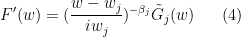
$\displaystyle F'(w) = (\frac{w-w_j}{iw_j})^{-\beta_j} \tilde G_j(w) \ \ \ \ \ (4)$

for ${w}$ near ${w_j}$ in ${D(0,1)}$ , for some ${\tilde G_j}$ that is also holomorphic and non-zero in a neighbourhood of ${w_j}$ in ${{\bf C}}$ .
The function ${F': D(0,1) \rightarrow {\bf C}}$ is holomorphic and non-vanishing; as ${D(0,1)}$ is simply connected, we must therefore have ${F' = \exp(H)}$ for some holomorphic ${H: D(0,1) \rightarrow {\bf C}}$ (by Exercise 47 of Notes 4). For any ${\theta}$ between ${\theta_j}$ and ${\theta_{j+1}}$ , we see from the previous discussion that ${F}$ extends holomorphically to a neighbourhood of ${e^{i\theta}}$ , with ${F'}$ non-vanishing at ${e^{i\theta}}$ , so ${H}$ extends also. From (3) we see that the argument of ${i e^{i\theta} \exp( H(e^{i\theta}) )}$ is constant on the interval ${(\theta_j, \theta_{j+1})}$ , and hence

$\displaystyle \theta + \mathrm{Im}( H(e^{i\theta})) \ \ \ \ \ (5)$

is also constant on this interval. Meanwhile, from (4) we see that for ${w}$ near ${w_j = e^{i\theta_j}}$ in ${D(0,1)}$ , we have

$\displaystyle H(w) = - \beta_j \mathrm{Log}_{I_-}( \frac{w-w_j}{iw_j}) + g_j(w)$

for some ${g_j}$ holomorphic in a neighbourhood of ${w_j}$ in ${{\bf C}}$ , where ${\mathrm{Log}_{I_-}}$ is a branch of the complex logarithm with branch cut at ${I_-}$ . From this we see that the function ${\theta \mapsto \theta + \mathrm{Im}( H(e^{i\theta}))}$ has a jump discontinuity with jump ${\beta_j \pi}$ as ${\theta}$ crosses ${\theta_j}$ . As this function clearly increases by ${2\pi}$ when ${\theta}$ increases by ${2\pi}$ , we conclude the geometric identity (2).
Now consider the modified function ${\tilde H: D(0,1) \rightarrow {\bf C}}$ defined by

$\displaystyle \tilde H(w) := H(w) + \sum_{j=1}^n \beta_j \mathrm{Log}_{I_-}( \frac{w-w_j}{iw_j}).$

Then ${\tilde H}$ is holomorphic on ${D(0,1)}$ , and by the above analysis it extends continuously to ${\overline{D(0,1)}}$ . We consider the imaginary part at ${w = e^{i\theta}}$ ,

$\displaystyle \mathrm{Im} \tilde H(e^{i\theta}) := \mathrm{Im} H(e^{i\theta}) + \sum_{j=1}^n \beta_j \mathrm{Arg}_{I_-}( \frac{e^{i\theta}-w_j}{iw_j}),$

where ${\mathrm{Arg}_{I_-}}$ is a branch of the argument function with branch cut at ${I_-}$ . Writing ${e^{i\theta} - w_j = 2 i e^{i(\theta+\theta_j)/2} \sin( (\theta - \theta_j)/2 )}$ , we see that ${\mathrm{Arg}_{I_-}( \frac{e^{i\theta}-w_j}{iw_j}) - \theta/2}$ is constant as long as ${\theta - \theta_j}$ is not an integer multiple of ${2\pi}$ . From this, (5), and (2), we see that the function ${\theta \mapsto \mathrm{Im} \tilde H(e^{i\theta})}$ is constant on each arc ${\theta_j < \theta < \theta_{j+1}}$ . Thus the function ${\mathrm{Im} \tilde H}$ is harmonic on ${D(0,1)}$ , continuous on ${\overline{D(0,1)}}$ , and constant on the boundary ${S^1}$ , so by the maximum principle it is constant, which from the Cauchy-Riemann equations makes ${\tilde H}$ constant also. Thus we have

$\displaystyle H(w) = c - \sum_{j=1}^n \beta_j \mathrm{Log}_{I_-}( \frac{w-w_j}{iw_j})$

on ${D(0,1)}$ for some complex constant ${c}$ , which on exponentiating gives

$\displaystyle F'(w) = \frac{C_1}{\prod_{j=1}^n ( \frac{w-w_j}{iw_j} )^{\beta_j} } \ \ \ \ \ (6)$

on ${D(0,1)}$ for some non-zero complex constant ${C_1}$ . Applying the fundamental theorem of calculus, we obtain the Schwarz-Christoffel formula:

Theorem 46 (Schwarz-Christoffel for the disk) Let ${\gamma_{z_1 \rightarrow \dots \rightarrow z_n \rightarrow z_1}}$ be a closed simple anticlockwise polygonal path, and define the exterior angles ${-1 < \beta_1,\dots,\beta_n < 1}$ as above. Let ${U}$ be the polygon enclosed by this path, and let ${F: D(0,1) \rightarrow U}$ be a complex diffeomorphism. Then there exist phases ${w_j = e^{i \pi \theta_j}}$ , ${j=1,\dots,n}$ for some ${\theta_1 < \dots < \theta_n < \theta_1+2}$ , a non-zero complex number ${C_1}$ , and a complex number ${C_2}$ such that

$\displaystyle F(w) = C_1 \int_0^w \frac{d\omega}{\prod_{j=1}^n ( \frac{\omega-w_j}{iw_j} )^{\beta_j} } + C_2$

for all ${w \in D(0,1)}$ , where the integral is over an arbitrary curve from ${0}$ to ${w}$ , and one selects a branch of ${z \mapsto z^{\beta_j}}$ with branch cut on the negative imaginary axis ${I_- := \{iy: y \geq 0\}}$ . Furthermore, ${F(w)}$ converges to ${z_j}$ as ${w}$ approaches ${w_j}$ for every ${1 \leq j \leq n}$ .

Note that one can change the branches of ${z \mapsto z^{\beta_j}}$ here, and also modify the normalising factors ${iw_j}$ , by adjusting the constant ${C_1}$ in a suitable fashion, as long one does not move the branch cut for ${\prod_{j=1}^n ( \frac{\omega-w_j}{iw_j} )^{\beta_j}}$ into the disk ${D(0,1)}$ ; one can similarly change the initial point ${0}$ of the curve to any other point in ${D(0,1)}$ by adjusting ${C_2}$ . By taking log-derivatives in (6), we can also express the Schwarz-Christoffel formula equivalently as a partial fractions decomposition of ${F''/F'}$ :

$\displaystyle \frac{F''(w)}{F'(w)} = \sum_{j=1}^n \frac{\beta_j}{w-w_j}.$

The Schwarz-Christoffel formula does not completely describe the conformal mappings from ${U}$ to the disk, because it does not specify exactly what the phases ${w_j}$ and the complex constants ${C_1,C_2}$ are. As the group of automorphisms ${z \mapsto e^{i\theta} \frac{z-\alpha}{1-\overline{\alpha}z}}$ of ${D(0,1)}$ has three degrees of freedom (one real parameter ${\theta}$ and one complex parameter ${\alpha}$ ), one can for instance fix three of the phases ${w_j}$ , but in general there are no simple formulae to then reconstruct the remaining parameters in the Schwarz-Christoffel formula, although numerical algorithms exist to compute them approximately. (In the case when the polygon is a rectangle, though, the Schwarz-Christoffel formula essentially produces an elliptic integral, and the complex diffeomorphisms from the rectangle to the disk or half-space are closely tied to elliptic functions; see Section 4.5 of Stein-Shakarchi for more discussion.)

Exercise 47 (Schwarz-Christoffel in a half-plane) Let ${\gamma_{z_1 \rightarrow \dots \rightarrow z_n \rightarrow z_1}}$ be a closed simple anticlockwise polygonal path, and define the exterior angles ${-1 < \beta_1,\dots,\beta_n < 1}$ as above. Let ${U}$ be the polygon enclosed by this path, and let ${F: {\bf H} \rightarrow U}$ be a complex diffeomorphism from the upper half-plane ${{\bf H} := \{ w \in {\bf C}: \mathrm{Im} w > 0 \}}$ to ${U}$ .

(i) Show that ${F}$ extends to a homeomorphism from the closure ${\overline{{\bf H}}}$ of the upper half-plane in the Riemann sphere to ${\overline{U}}$ , and that ${f(z_1),\dots,f(z_n)}$ all lie on ${{\bf R} \cup \{\infty\}}$ , where ${f: \overline{U} \rightarrow {\bf H}}$ is the inverse of the extension of ${F}$ .

(ii) If all of the ${f(z_1),\dots,f(z_n)}$ are finite, show that after a cyclic permutation one has ${f(z_1) < \dots < f(z_n)}$ , and that there exists a non-zero complex number ${C_1}$ , and a complex number ${C_2}$ such that
$\displaystyle F(w) = C_1 \int_i^w \frac{d\omega}{\prod_{j=1}^{n} ( \omega-f(z_j) )^{\beta_j} } + C_2$

for all ${w \in {\bf H}}$ , where the integral is over any curve from ${i}$ to ${w}$ in ${{\bf H}}$ .

(iii) If one of the ${f(z_1),\dots,f(z_n)}$ are infinite, show after a cyclic permutation that one has ${f(z_1) < \dots < f(z_{n-1})}$ and ${f(z_n) = \infty}$ , and there exists a non-zero complex number ${C_1}$ , and a complex number ${C_2}$ such that
$\displaystyle F(w) = C_1 \int_i^w \frac{d\omega}{\prod_{j=1}^{n-1} ( \omega-f(z_j) )^{\beta_j} } + C_2$

for all ${w \in {\bf H}}$ .

Remark 48 One could try to apply the Schwarz-Christoffel formula to a closed polygonal path ${\gamma_{z_1 \rightarrow \dots \rightarrow z_n \rightarrow z_1}}$ that is not simple. In such cases (and after choosing the parameters ${C_1,C_2,w_1,\dots,w_n}$ correctly), what tends to happen is that the map ${F}$ still maps the circle ${S^1}$ to the closed path, but fails to be injective.

Exercise 49 Let ${F: P \rightarrow {\bf H}}$ be a complex diffeomorphism from the half-strip ${P := \{ z \in {\bf C}: \mathrm{Im} z > 0; -\frac{\pi}{2} < \mathrm{Re} z < \frac{\pi}{2} \}}$ to the upper half-plane ${{\bf H}}$ , which extends to a continuous map ${F: \overline{P} \rightarrow \overline{{\bf H}}}$ to the closures of ${P}$ , ${{\bf H}}$ in the Riemann sphere. Suppose that ${F}$ maps ${-\frac{\pi}{2}, \frac{\pi}{2}, \infty}$ to ${-1,1,\infty}$ respectively. Show that ${F'(w) = \frac{1}{(1-w^2)^{1/2}}}$ , where we take the branch of the square root that is positive on the real axis and has a branch cut at ${I_-}$ . (Hint: ${P}$ is not quite a polygon, so one cannot directly apply the Schwarz-Christoffel formula; however the proof of that formula will still apply.)
There is a simple description of ${F}$ in terms of trigonometric functions. What is it?

— 5. The uniformisation theorem (optional) —

Now we discuss a proof of the uniformisation theorem, Theorem 5, following the approach in these notes of Marshall. Unfortunately the argument is rather complicated, and we will only give a portion of the proof here. One of the many difficulties in trying to prove this theorem is the fact that the conclusion is a disjunction of three alternatives, each with a rather different complex geometry; it would be easier if there was only one target geometry that one was trying to impose on the Riemann surface ${M}$ . To begin separating the three geometries from each other, recall from Liouville’s theorem that there are no non-constant bounded holomorphic functions on ${{\bf C}}$ or ${{\bf C} \cup \{\infty\}}$ , but plenty of non-constant bounded holomorphic functions on ${D(0,1)}$ . By Lemma 1, the same claims hold for Riemann surfaces that are complex diffeomorphic to ${{\bf C}}$ or ${{\bf C} \cup \{\infty\}}$ or to ${D(0,1)}$ respectively. Note that without loss of generality we may normalise “bounded” by replacing it with “mapping into ${D(0,1)}$ “. From this we see that the uniformisation theorem can be broken up into two simpler pieces:

Theorem 50 (Uniformisation theorem, hyperbolic case) Let ${M}$ be a simply connected Riemann surface that admits a non-constant holomorphic map from ${M}$ to ${D(0,1)}$ . Then ${M}$ is complex diffeomorphic to ${D(0,1)}$ .

Theorem 51 (Uniformisation theorem, non-hyperbolic case) Let ${M}$ be a simply connected Riemann surface that does not admit a non-constant holomorphic map from ${M}$ to ${D(0,1)}$ . Then ${M}$ is complex diffeomorphic to ${{\bf C}}$ or ${{\bf C} \cup \{\infty\}}$ .

Let us now focus on the hyperbolic case of the uniformisation theorem, Theorem 50. Now we do not have the disjunction problem as there is only one target geometry to impose on ${M}$ ; we will be able to give a complete proof of this theorem here (in contrast to Theorem 51, where we will only give part of the proof). Let ${p_0}$ be a point in ${M}$ , and recall that ${{\mathcal H}_{p_0}}$ denotes the collection of holomorphic maps ${f: M \rightarrow D(0,1)}$ that maps ${p_0}$ to ${0}$ . By hypothesis (and applying a suitable automorphism of ${D(0,1)}$ ), ${{\mathcal H}_{p_0}}$ contains at least one non-constant map. If Theorem 50 were true, then from Lemma 39 we see that ${{\mathcal H}_{p_0}}$ would contain a “maximal” element ${\phi}$ which would exhibit the desired complex diffeomorphism between ${M}$ and ${D(0,1)}$ .

It turns out that the converse statement is true: if we can locate “maximal” elements of ${{\mathcal H}_{p_0}}$ with certain properties, then we can prove Theorem 50. More precisely, Theorem 50 can be readily deduced from the following claim.

Theorem 52 (Maximal maps into ${D(0,1)}$ ) Let ${M}$ be a simply connected Riemann surface, let ${p_0}$ be a point in ${M}$ , and let ${{\mathcal H}_{p_0}}$ be the collection of holomorphic maps from ${M}$ to ${D(0,1)}$ that map ${p_0}$ to ${0}$ . Suppose that ${{\mathcal H}_{p_0}}$ contains a non-constant map. Then ${{\mathcal H}_{p_0}}$ contains a map ${\phi_{p_0}: M \rightarrow D(0,1)}$ with the property that ${|f(p)| \leq |\phi_{p_0}(p)|}$ for all ${p \in M \backslash \{p_0\}}$ and ${f \in {\mathcal H}_{p_0}}$ , with equality only if ${f = e^{i\theta} \phi_{p_0}}$ for some real number ${\theta}$ . Furthermore ${\phi_{p_0}}$ has a simple zero at ${p_0}$ , and no other zeroes.

We have seen how Theorem 50 implies Theorem 52. Let us now demonstrate the converse implication, assuming Theorem 52 for the moment and deriving Theorem 50. Let ${M}$ be a simply connected Riemann surface that admits non-constant holomorphic maps from ${M}$ to ${D(0,1)}$ , and pick a point ${p_0}$ in ${M}$ . By applying a suitable automorphism of ${D(0,1)}$ we see that ${{\mathcal H}_{p_0}}$ has a non-constant map, so by Theorem 52 this collection contains an element ${\phi_{p_0}}$ with the stated properties. Now let ${p_0,p_1}$ be two points in ${M}$ . Since ${\phi_{p_0}}$ has a zero only at ${p_0}$ , we thus have ${\phi_{p_0}(p_1) = \phi_{p_0}(p_2) \neq 0}$ for some distinct ${p_1, p_2 \in M \backslash \{p_0\}}$ . Let ${R: D(0,1) \rightarrow D(0,1)}$ be the automorphism

$\displaystyle R(z) := \frac{z - \phi_{p_0}(p_1)}{1 - \overline{\phi_{p_0}(p_1)} z}$

that maps ${\phi_{p_0}(p_1)}$ to ${0}$ and ${0}$ to ${-\phi_{p_0}(p_1)}$ , then the function ${R \circ \phi_{p_0}: M \rightarrow D(0,1)}$ lies in ${{\mathcal H}_{p_1}}$ and also has a zero at ${p_2}$ . From Theorem 52, we thus have

$\displaystyle |R \circ \phi_{p_0}(p_0)| \leq |\phi_{p_1}(p_0)|;$

since ${\phi_{p_0}(p_0)}$ vanishes, we thus have from the definition of ${R}$ that

$\displaystyle |\phi_{p_0}(p_1)| \leq |\phi_{p_1}(p_0)|.$

Swapping the roles of ${p_0}$ and ${p_1}$ gives the reverse inequality, thus we in fact have

$\displaystyle |R \circ \phi_{p_0}(p_0)| = |\phi_{p_1}(p_0)|$

and

$\displaystyle |\phi_{p_0}(p_1)| =|\phi_{p_1}(p_0)|. \ \ \ \ \ (7)$

Applying Theorem 52 again, we conclude that

$\displaystyle R \circ \phi_{p_0} = e^{i\theta} \phi_{p_1} \ \ \ \ \ (8)$

for some ${\theta \in {\bf R}}$ .
Using this identity, we can now show that each of the ${\phi_{p_0}}$ are injective. Indeed, if ${\phi_{p_0}}$ was not injective, then we must have ${\phi_{p_0}(p_1) = \phi_{p_0}(p_2)}$ for some distinct ${p_1,p_2 \in M}$ , neither of which can equal ${p_0}$ since ${\phi_{p_0}}$ has no other zeroes than ${p_0}$ . But then by (8) we see that ${\phi_{p_1}(p_2) = \phi_{p_1}(p_1) = 0}$ , contradicting the fact that ${\phi_{p_1}}$ has a zero only at ${p_1}$ . Thus ${\phi_{p_0}}$ is indeed injective. Applying Proposition 41 we conclude that ${M}$ and ${D(0,1)}$ were complex diffeomorphic. This concludes the derivation of Theorem 50 from Theorem 52.

Remark 53 We only established that ${\phi_{p_0}: M \rightarrow D(0,1)}$ was injective in the above argument, but by inspecting the proof of Proposition 41 and using the maximality properties of ${\phi_{p_0}}$ we see that ${\phi_{p_0}}$ is also surjective, and thus supplies the required complex diffeomorphism between ${M}$ and ${D(0,1)}$ . In a similar vein, the arguments in the preceding section show that under the hypotheses of Theorem 50, there exists a surjective map from ${M}$ to ${D(0,1)}$ , but one needs something like Theorem 52 to obtain the crucial additional property of injectivity (which was automatic in the preceding section, since one already started with an injection in hand).

To finish off the hyperbolic case of the uniformisation theorem, it remains to prove Theorem 52. It is convenient to work with harmonic functions instead of holomorphic functions. Observe that if ${\phi_{p_0}: M \rightarrow D(0,1)}$ were holomorphic with a simple zero at ${p_0}$ but no other zeroes, then we have local holomorphic branches of ${\log \frac{1}{\phi_{p_0}}}$ on small neighbourhoods of any point in ${M \backslash \{p_0\}}$ . Taking real parts, we conclude that the function ${g_{p_0} := \log \frac{1}{|\phi_{p_0}|}: M \backslash \{p_0\} \rightarrow {\bf R}}$ is harmonic on the punctured surface ${M \backslash \{p_0\}}$ ; it is also positive since ${\phi_{p_0}}$ takes values in ${D(0,1)}$ . Furthermore, the function ${g_{p_0}}$ has a logarithmic singularity at ${p_0}$ in the following sense: if ${z: U_{p_0} \rightarrow D(0,1)}$ was any coordinate chart on some neighbourhood ${U_{p_0}}$ of ${p_0}$ that mapped ${p_0}$ to ${D(0,1)}$ , then as ${\phi_{p_0}}$ had a simple zero at ${p_0}$ , the function ${\log \frac{1}{|\phi_{p_0}|} - \log \frac{1}{|z|}}$ , defined on ${U_{p_0} \backslash \{p_0\}}$ , stays bounded as one approaches ${p_0}$ .

Conversely, one can reconstruct ${\phi_{p_0}}$ from ${g_{p_0}}$ (up to a harmless phase ${e^{i\theta}}$ ) by the following lemma.

Lemma 54 (Reconstructing a holomorphic function from its magnitude) Let ${M}$ be a simply connected Riemann surface, let ${p_0}$ be a point in ${M}$ , and let ${g_{p_0}: M \backslash \{p_0\} \rightarrow {\bf R}}$ be harmonic. Suppose that ${g_{p_0}}$ has a logarithmic singularity at ${p_0}$ in the sense that ${g_{p_0} - \log \frac{1}{|z|}}$ is bounded near ${p_0}$ for some coordinate chart ${z: U_{p_0} \rightarrow D(0,1)}$ on a neighbourhood ${U_{p_0}}$ of ${p_0}$ that maps ${p_0}$ to ${0}$ . Then there exists a holomorphic function ${\phi: M \rightarrow {\bf C}}$ with a simple zero at ${p_0}$ and no other zeroes, such that ${g_{p_0} = \log \frac{1}{|\phi|}}$ on ${M \backslash \{p_0\}}$ .

Proof: Let ${g_{p_0}}$ be as above. Call a function ${\phi: U \rightarrow {\bf C}}$ on an open subset ${U}$ of ${M}$ good if it is holomorphic with ${g_{p_0} = \log \frac{1}{|\phi|}}$ on ${U \backslash \{p_0\}}$ (in particular this forces ${\phi}$ to be non-zero away from ${p_0}$ ), and has a simple zero at ${p_0}$ if ${p_0}$ lies in ${U}$ . Clearly it will suffice to find a good function on all of ${M}$ .

We first solve the local problem, showing that for any ${p \in M}$ there exists a neighbourhood ${U_p}$ of ${p}$ that supports a good function ${\phi_p: U_p \rightarrow {\bf C}}$ . If ${p \neq p_0}$ , we can work in a chart ${U_p}$ avoiding ${p_0}$ which is diffeomorphic to a disk ${D(0,1)}$ . If we identify ${U_p}$ with ${D(0,1)}$ then ${g_{p_0}}$ restricted to ${U_p}$ can be viewed as a harmonic function on ${D(0,1)}$ . As this disk is simply connected, ${g}$ will have a harmonic conjugate and is thus the real part of a holomorphic function ${f}$ on this disk. Taking ${\phi_p}$ to be ${e^{-f}}$ we obtain the required good function. Now suppose instead that ${p = p_0}$ . Using the coordinate chart ${z: U_{p_0} \rightarrow D(0,1)}$ to identify ${U_{p_0}}$ with ${D(0,1)}$ , we now have a harmonic function ${g_{p_0}: D(0,1) \backslash \{0\} \rightarrow {\bf R}}$ with ${g_{p_0} - \log\frac{1}{|z|}}$ bounded near zero. Applying Exercise 60 of Notes 4, we conclude that ${g_{p_0} - \log\frac{1}{|z|}}$ extends to a harmonic function ${h}$ on ${D(0,1)}$ , which is then the real part of a holomorphic function ${f}$ ; taking ${\phi_{p_0} := z e^{-f}}$ then gives a good function on ${U_{p_0}}$ .

Next, we make the following compatibility observation: if ${\phi: U \rightarrow {\bf R}}$ and ${\psi: V \rightarrow {\bf R}}$ are both good functions, then ${\phi/\psi}$ is constant on every connected component of ${U \cap V}$ (after removing any singularity at ${p_0}$ ). Indeed, by construction ${\phi/\psi}$ is holomorphic and of magnitude one, so locally there are holomorphic branches of ${\log(\phi/\psi)}$ that have vanishing real part, hence locally constant imaginary part by the Cauchy-Riemann equations. Hence ${\phi/\psi}$ is locally constant as claimed.

Now we need to glue together the local good functions into a global good function. This is a “monodromy problem”, which can be solved using analytic continuation and the simply connected nature of ${M}$ by the following “monodromy theorem” argument. Let us pick a good function ${\phi_{p_0}: U_{p_0} \rightarrow {\bf R}}$ on some neighbourhood of ${p_0}$ . Given any other point ${p}$ in ${M}$ , we can form a path ${\gamma: [0,1] \rightarrow M}$ from ${p_0}$ to ${p}$ . We claim that for any ${0 \leq T \leq 1}$ , we can find a finite sequence ${0 = t_0 < t_1 < \dots < t_n = T}$ and good functions ${\phi_j: U_j \rightarrow {\bf R}}$ for ${j=1,\dots,n}$ such that each ${U_j}$ contains ${\gamma([t_{j-1},t_j])}$ , and such that ${\phi_j}$ and ${\phi_{j+1}}$ agree on a neighbourhood of ${\gamma(t_j)}$ for each ${j=1,\dots,n-1}$ , and ${\phi_1}$ and ${\phi_{p_0}}$ also agree on a neighbourhood of ${\gamma(t_0)}$ . The set ${\Omega}$ of such ${T}$ is easily seen to be an open non-empty subset of ${[0,1]}$ . Now we claim that it is closed. Suppose that ${T_k \in \Omega}$ converges to a limit ${T_* \in \Omega}$ as ${k \rightarrow \infty}$ . If any of the ${T_k}$ are greater than or equal to ${T_*}$ it is easy to see that ${T_* \in \Omega}$ , so suppose instead that the ${T_k}$ are all less than ${T_*}$ . We take a good function ${\psi_*: U_* \rightarrow {\bf R}}$ supported on some neighbourhood ${U_*}$ of ${\gamma(T_*)}$ . By continuity, ${U_*}$ will contain ${\gamma([T_k,T_*])}$ for some sufficiently large ${k}$ . We would like to append ${\psi_*}$ and ${U_*}$ to the sequence of good functions ${\phi_j: U_j \rightarrow {\bf R}}$ , ${j=1,\dots,k}$ one obtains from the hypothesis ${T_k \in \Omega}$ , but there is the issue that ${\psi_*}$ need not agree with ${\phi_k}$ at the endpoint ${\gamma(T_k)}$ . However, they only differ by a constant of magnitude one near this endpoint, so after multiplying ${\psi_*}$ by an appropriate constant of magnitude one, we can conclude that ${T_*\in \Omega}$ as claimed.

By the continuity method, ${\Omega}$ is all of ${[0,1]}$ , and in particular contains ${1}$ . Thus we can find ${0 = t_0 < t_1 < \dots < t_n = 1}$ and good functions ${\phi_j: U_j \rightarrow {\bf R}}$ for ${j=1,\dots,n}$ such that each ${U_j}$ contains ${\gamma([t_{j-1},t_j])}$ , and such that ${\phi_j}$ and ${\phi_{j+1}}$ agree on a neighbourhood of ${\gamma(t_j)}$ for each ${j=1,\dots,n-1}$ , and ${\phi_1}$ and ${\phi_{p_0}}$ also agree on a neighbourhood of ${\gamma(t_0)}$ . Consider the final value ${\phi_n(p)}$ obtained by the last good function ${\phi_n: U_n \rightarrow {\bf R}}$ at the endpoint ${\gamma(t_n) = p}$ of the curve ${\gamma}$ . From analytic continuation and a continuity argument we see that if we perform a homotopy of ${\gamma}$ with fixed endpoints, this final value does not change (even if the number ${n}$ of good functions may vary). Thus we can define a function ${\phi: M \rightarrow {\bf R}}$ by setting ${\phi(p) := \phi_n(p)}$ whenever ${\gamma}$ is a path from ${p_0}$ to ${p}$ and ${\phi_n}$ is the final good function constructed by the above procedure. From construction we see that ${\phi}$ is locally equal to a good function at every point in ${M}$ , and is thus itself a good function, as required. $\Box$

Exercise 55 (Monodromy theorem) Let ${M}$ be a simply connected Riemann surface, let ${N}$ be another Riemann surface, let ${p_0}$ be a point in ${M}$ , let ${U_{p_0}}$ be an open neighbourhood of ${p_0}$ , and let ${\phi_{p_0}: U_{p_0} \rightarrow N}$ be holomorphic. Prove that the following statements are equivalent.

(i) ${\phi_{p_0}}$ has a holomorphic extension to ${M}$ ; that is to say, there is a holomorphic function ${f: M \rightarrow N}$ whose restriction to ${U_{p_0}}$ is equal to ${\phi_{p_0}}$ .

(ii) For every curve ${\gamma: [0,1] \rightarrow M}$ starting at ${p_0}$ , we can find ${0 = t_0 < t_1 < \dots < t_n = 1}$ and holomorphic functions ${\phi_j: U_j \rightarrow N}$ for ${j=0,\dots,n}$ with ${\phi_0 = \phi_{p_0}}$ , such that ${U_j}$ is an open subset of ${M}$ containing ${\gamma([t_j,t_{j+1}])}$ , and ${\phi_j}$ and ${\phi_{j+1}}$ agree on a neighbourhood of ${\gamma(t_j)}$ for each ${j=0,\dots,n-1}$ .

Furthermore, if (i) holds, show that the holomorphic extension ${f: M \rightarrow N}$ is unique. Give a counterexample that shows that the monodromy theorem fails if ${M}$ is only assumed to be connected rather than simply connected.

We remark that while the condition (ii) in the monodromy theorem looks somewhat complicated, it becomes more geometrically natural if one adopts the language of sheaves, which we will not do here.

In view of Lemma 54, we may reduce the task of establishing Theorem 52 to that of establishing the existence of a special type of harmonic function on ${M}$ (with one point ${p_0}$ removed), namely a Green’s function:

Definition 56 (Green’s function) Let ${M}$ be a connected Riemann surface, and let ${p_0}$ be a point in ${M}$ . A Green’s function for ${M}$ at ${p_0}$ is a function ${g_{p_0}: M \backslash \{p_0\} \rightarrow {\bf R}}$ with the following properties:

(i) ${g_{p_0}}$ is harmonic on ${M \backslash \{p_0\}}$ .

(ii) ${g_{p_0}}$ is non-negative on ${M \backslash \{p_0\}}$ .

(iii) ${g_{p_0}}$ has a logarithmic singularity at ${p_0}$ in the sense that ${g_{p_0} - \log \frac{1}{|z|}}$ is bounded near ${p_0}$ for some coordinate chart ${z: U_{p_0} \rightarrow D(0,1)}$ that maps ${p_0}$ to ${0}$ .

(iv) ${g_{p_0}}$ is minimal with respect to the properties (i)-(iii), in the sense that for any other ${g'_{p_0}: M \backslash \{p_0\} \rightarrow {\bf R}}$ obeying (i)-(iii), we have ${g_{p_0} \leq g'_{p_0}}$ pointwise in ${M \backslash \{p_0\}}$ .

Clearly if a Green’s function for ${M}$ at ${p_0}$ exists, it is unique by property (iv), so we can talk about the Green’s function for ${M}$ at ${p_0}$ , if it exists. In the case of the disk ${D(0,1)}$ , a Greens’ function may be explicitly computed:

Exercise 57 If ${\alpha \in D(0,1)}$ , show that the function ${g_\alpha: D(0,1) \rightarrow {\bf R}}$ defined by ${g_\alpha(z) := \log \frac{|1-\overline{\alpha} z|}{|z-\alpha|}}$ is a Green’s function for ${D(0,1)}$ at ${\alpha}$ .

Theorem 52 may now be deduced from the following claim.

Proposition 58 (Existence of Green’s function) Let ${M}$ be a connected Riemann surface, let ${p_0}$ be a point in ${M}$ , and suppose that the collection ${{\mathcal H}_{p_0}}$ of holomorphic maps ${f: M \rightarrow D(0,1)}$ that map ${p_0}$ to ${0}$ contains at least one non-constant map. Then the Green’s function ${g_{p_0}: M \backslash \{p_0\} \rightarrow {\bf R}}$ for ${M}$ at ${p_0}$ exists. Furthermore, for any ${f \in {\mathcal H}_{p_0}}$ , one has ${|f(p)| \leq e^{-g_{p_0}(p)}}$ for any ${p \in M \backslash \{p_0\}}$ .

(Note that in this proposition we no longer need ${M}$ to be simply connected.) Indeed, suppose that Proposition 58 held. Let ${M}$ be a simply connected Riemann surface, and let ${p_0 \in M}$ with ${{\mathcal H}_{p_0}}$ containing a non-constant map. By hypothesis, the Green’s function ${g_{p_0}}$ is non-negative on ${M \backslash \{p_0\}}$ . Noting that ${M}$ remains connected if we remove a small disk around ${p_0}$ , and from (iii) that ${g_{p_0}}$ will be strictly positive on the boundary of that disk, we observe from the maximum principle (Exercise 18) and (ii) that ${g_{p_0}}$ is in fact strictly positive on ${M \backslash \{p_0\}}$ . By Lemma 54 we can find a holomorphic function ${\phi_{p_0}: M \rightarrow {\bf C}}$ with a simple zero at ${p_0}$ and no other zeroes, such that ${|\phi_{p_0}| = e^{-g_{p_0}}}$ on ${M \backslash \{p_0\}}$ . As ${g_{p_0}}$ is strictly positive, ${\phi_{p_0}}$ takes values in ${D(0,1)}$ and is thus in ${{\mathcal H}_{p_0}}$ . From Proposition 58 we see that ${|f(p)| \leq |\phi_{p_0}(p)|}$ for all ${p \in M \backslash \{p_0\}}$ . If equality occurs anywhere, then the quotient ${f/\phi_{p_0}}$ (after removing the singularity) is a function taking values in the closed unit disk ${\overline{D(0,1)}}$ , which has magnitude ${1}$ at ${p}$ ; by the maximum principle (or open mapping theorem) we then have ${f/\phi_{p_0} = e^{i\theta}}$ for some real ${\theta}$ . Thus ${\phi_{p_0}}$ obeys all the properties required for Theorem 52.

It remains to obtain the existence of the Green’s function ${g_{p_0}}$ . To do this, we use a powerful technique for constructing harmonic functions, known as Perron’s method of subharmonic functions. The basic idea is to build a harmonic function by taking a suitable large family of subharmonic functions and then forming their supremum. We first give a definition of subharmonic function.

Definition 59 (Subharmonic function) Let ${M}$ be a Riemann surface. A subharmonic function on ${M}$ is an upper semi-continuous function ${u: M \rightarrow {\bf R} \cup \{-\infty\}}$ obeying the following upper maximum principle: for any connected compact set ${K}$ in ${M}$ with non-empty boundary and any function ${v: K \rightarrow {\bf R}}$ that is continuous on ${K}$ and harmonic on the interior of ${K}$ , if ${u(p) \leq v(p)}$ for all ${p \in \partial K}$ , then ${u(p) \leq v(p)}$ for all ${p \in K}$ .
A superharmonic function is similarly defined as a lower semi-continuous function ${u: M \rightarrow {\bf R} \cup \{+\infty\}}$ such that for any connected compact ${K \subset M}$ with non-empty boundary and any function ${v: K \rightarrow {\bf R}}$ continuous on ${K}$ and harmonic on the interior of ${K}$ , the bound ${u(p) \geq v(p)}$ for ${p \in \partial K}$ implies that ${u(p) \geq v(p)}$ for all ${p \in K}$ .

Clearly subharmonicity and superharmonicity are conformal invariants in the sense that the analogue of Lemma 1 holds for these concepts. We have the following elementary properties of subharmonic functions and superharmonic functions:

Exercise 60 Let ${M}$ be a Riemann surface.

(i) Show that a function ${u: M \rightarrow {\bf R} \cup \{-\infty\}}$ is subharmonic if and only if ${-u}$ is superharmonic.

(ii) Show that a function ${u: M \rightarrow {\bf R}}$ is harmonic if and only if it is both subharmonic and superharmonic.

(iii) If ${u,v: M \rightarrow {\bf R} \cup \{-\infty\}}$ are subharmonic, show that ${\max(u,v)}$ is also.

(iv) Let ${u: M \rightarrow {\bf R} \cup \{-\infty\}}$ be subharmonic, and let ${U}$ be an open subset of ${M}$ . Show that the restriction of ${u}$ to ${U}$ is subharmonic.

(v) (Subharmonicity is a local property) Conversely, let ${u: M \rightarrow {\bf R} \cup \{-\infty\}}$ is subharmonic, and suppose that for each ${p \in M}$ there is a neighbourhood ${U_p}$ of ${p}$ such that the restriction of ${u}$ to ${U_p}$ is subharmonic. Show that ${u}$ is itself subharmonic. (Hint: If ${v}$ is continuous on a connected compact set ${K}$ with non-empty boundary and harmonic on the interior, and ${v-u}$ attains a minimum at an interior point of ${K}$ , show that ${v-u}$ is constant in some neighbourhood of that point. Exercise 43 may come in handy, as well as the fact (which you can use without proof) that upper (resp. lower) semi-continuous functions on a compact subset of ${{\bf C}}$ can be expressed as the pointwise limit of a decreasing (resp. increasing) sequence of continuous functions.)

(vi) (Maximum principle) Let ${u: M \rightarrow {\bf R} \cup \{-\infty\}}$ be subharmonic, let ${v: M \rightarrow {\bf R} \cup \{+\infty\}}$ be superharmonic, and let ${K}$ be a connected compact subset of ${M}$ with non-empty boundary such that ${u(p) \leq v(p)}$ for all ${p \in \partial K}$ . Show that ${u(p) \leq v(p)}$ for all ${p \in K}$ . (This is a similar argument to (v).)

(vii) Show that the sum of two subharmonic functions is again subharmonic (using the usual conventions on adding ${-\infty}$ to itself or to another real number).

(viii) (Harmonic patching) Let ${u: M \rightarrow {\bf R} \cup \{-\infty\}}$ be subharmonic, let ${K}$ be connected compact with non-empty boundary, and let ${v: K \rightarrow {\bf R}}$ be a continuous function on ${K}$ that is harmonic on the interior of ${K}$ and agrees with ${u}$ on the boundary of ${K}$ . Show that the function ${\tilde u: M \rightarrow {\bf R} \cup \{-\infty\}}$ , defined to equal ${v}$ on ${K}$ and ${u}$ on ${M \backslash K}$ , is subharmonic.

(ix) Let ${f: M \rightarrow {\bf C}}$ be a holomorphic function. Show that ${\log |f|}$ is subharmonic, with the convention that ${\log 0 = -\infty}$ . (Hint: first use the maximum principle and harmonic conjugates to show that if ${M}$ contains a copy of a closed disk ${\overline{D(z_0,r)}}$ , and ${\log |f| \leq u}$ on the boundary of this disk for some continuous ${u: \overline{D(z_0,r)} \rightarrow {\bf R}}$ that is harmonic in the interior of the disk, then ${\log |f| \leq u}$ in the interior of the disk also.)

For smooth functions on an open subset of ${{\bf C}}$ , one can express the property of subharmonicity quite explicitly:

Exercise 61 Let ${U}$ be an open subset of ${{\bf C}}$ , and let ${u: U \rightarrow {\bf R}}$ be continuously twice (Fréchet) differentiable. Show that the following are equivalent:

(i) ${u}$ is subharmonic.

(ii) For all closed disks ${\overline{D(z_0,r)}}$ in ${U}$ , one has
$\displaystyle u(z_0) \leq \frac{1}{2\pi} \int_0^{2\pi} u(z_0+re^{i\theta})\ d\theta.$

(iii) One has ${\Delta u(z_0) \geq 0}$ for all ${z_0 \in U}$ .

Show that the equivalence of (i) and (ii) in fact holds even if ${u}$ is only assumed to be continuous rather than continuously twice differentiable.

However, we will not use the above exercise in our analysis here as it will not be convenient to impose a hypothesis of continuous twice differentiability on our subharmonic functions. For instance, in the unit disk ${D(0,1)}$ , the function ${\log |z|}$ is an example of a subharmonic function that attains the value ${-\infty}$ at the origin. A more sophisticated example is ${\sum_{k=2}^\infty \frac{1}{k^2} \log |z-1/k|}$ , which is also subharmonic but is now discontinuous at the origin (even if one uses the topology of the extended reals).

The Perron method is based on the observation that under certain conditions, the supremum of a family of subharmonic functions is not just subharmonic (as per Exercise 60(iii)), but is in fact harmonic. A key concept here is that of a Perron family:

Definition 62 Let ${M}$ be a Riemann surface. A continuous Perron family on ${M}$ is a family ${{\mathcal F}}$ of continuous subharmonic functions ${u: M \rightarrow {\bf R}}$ with the following properties:

(i) If ${u, v \in {\mathcal F}}$ , then ${\max(u,v) \in {\mathcal F}}$ .

(ii) (Harmonic patching) If ${u \in {\mathcal F}}$ , ${K}$ is a connected compact subset of ${M}$ with non-empty boundary, and ${v: K \rightarrow {\bf R}}$ is a continuous function that is harmonic in the interior of ${K}$ and equals ${u}$ on the boundary of ${K}$ , then the function ${\tilde u: M \rightarrow {\bf R}}$ defined to equal ${v}$ on ${K}$ and ${u}$ outside of ${K}$ also lies in ${{\mathcal F}}$ .

One can also consider more general Perron families of subharmonic functions that are merely upper semi-continuous rather than continuous, but for the current application continuous Perron families will suffice.

The fundamental theorem that powers the Perron method is then

Theorem 63 (Perron method) Let ${{\mathcal F}}$ be a non-empty continuous Perron family on a connected Riemann surface ${M}$ , and set ${u: M \rightarrow {\bf R} \cup \{+\infty\}}$ to be the function ${u(p) := \sup_{v \in {\mathcal F}} v(p)}$ . Then one of the following two statements hold:

(i) ${u(p) = +\infty}$ for all ${p \in M}$ .

(ii) ${u}$ is a harmonic function on ${M}$ .

Proof: Let us first work locally in some open subset ${U}$ of ${M}$ that is complex diffeomorphic to a disk ${D(0,1)}$ ; to simplify the discussion we abuse notation by identifying ${U}$ with ${D(0,1)}$ in the following discussion.

Assume for the moment that ${u}$ is not identically equal to ${+\infty}$ on ${D(0,1/2)}$ . Let ${p_0}$ be an arbitrary point in ${D(0,1/2)}$ (viewed as a subset of ${U}$ ). Then we can find a sequence ${u_n \in {\mathcal F}}$ such that ${u_n(p_0) \rightarrow u(p_0)}$ as ${n \rightarrow \infty}$ .

We can use Exercise 43 to find a continuous function ${v_1: \overline{D(0,1/2)} \rightarrow {\bf R} \cup \{-\infty\}}$ that equals ${u_1}$ on the boundary of this disk (viewed as a subset of ${U}$ ) and is harmonic and at least as large as ${u_1}$ in the interior; if we then let ${\tilde u_1}$ be the function defined to equal ${v_1}$ on ${\overline{D(0,1/2)}}$ and ${u_1}$ outside of this disk, then ${\tilde u_1}$ is larger than ${u_1}$ and also lies in ${{\mathcal F}}$ thanks to axiom (ii). Thus, by replacing ${u_1}$ with ${\tilde u_1}$ , we may assume that ${u_1}$ is harmonic on ${D(0,1/2)}$ . Next, by replacing ${u_2}$ with ${\max(u_1,u_2)}$ and using axiom (i), we may assume that ${u_1 \leq u_2}$ pointwise; replacing ${u_2}$ with a harmonic function on ${D(0,1/2)}$ as before we may assume that ${u_2}$ is harmonic on ${D(0,1/2)}$ . Continuing in this fashion we may assume that ${u_1 \leq u_2 \leq \dots}$ and that ${u_1,u_2,\dots}$ are harmonic on ${D(0,1/2)}$ . Form the function ${w_{p_0} := \sup_n u_n}$ , then we have ${w_{p_0} \leq u}$ pointwise with ${w_{p_0}(p_0) = u(p_0)}$ . By the Harnack principle (Exercise 59 of Notes 4), we thus see that ${w_{p_0}}$ is either harmonic on ${D(0,1/2)}$ , or equal to ${+\infty}$ on ${D(0,1/2)}$ . The latter cannot occur since we are assuming ${u}$ not identically equal to ${+\infty}$ , thus ${w_{p_0}}$ is harmonic.

Now let ${p_1}$ be another point in ${D(0,1/2)}$ . We can find another sequence ${u'_n \in {\mathcal F}}$ with ${u'_n(p_1) \rightarrow u(p_1)}$ . As before we may assume that the ${u'_n}$ are increasing and are harmonic on ${D(0,1/2)}$ ; we may also assume that ${u'_n \geq u_n}$ pointwise. Setting ${w_{p_1} := \sup_n u'_n}$ , we conclude that ${w_{p_1}}$ is harmonic with ${w_{p_0} \leq w_{p_1} \leq u}$ on ${D(0,1/2)}$ . In particular ${w_{p_0}(p_0) = w_{p_1}(p_0)}$ . The harmonic function ${w_{p_1}-w_{p_0}}$ is non-negative on ${D(0,1/2)}$ and vanishes at ${p_0}$ , hence is identically zero on ${D(0,1/2)}$ by the maximum principle. Since ${w_{p_1}(p_1) = u(p_1)}$ , we conclude that ${w_{p_0}}$ and ${u}$ agree at ${p_1}$ . Since ${p_1}$ was an arbitrary point on ${D(0,1/2)}$ , we conclude that ${u=w_{p_0}}$ is harmonic at ${D(0,1/2)}$ .

Putting all this together, we see that for any point ${p}$ in ${M}$ there is a neighbourhood ${U_p}$ (corresponding to the disk ${D(0,1/2)}$ in the above arguments) with the property that ${u}$ is either equal to ${+\infty}$ on ${U_p}$ , or is harmonic on ${U_p}$ . By a continuity argument we conclude that one of the two options (i), (ii) of the theorem must hold. $\Box$

Now we can conclude the proof of Proposition 58, and hence the hyperbolic case of the uniformisation theorem, by applying the above theorem to a well-chosen Perron family. Let ${M}$ be a simply connected Riemann surface, and let ${{\mathcal F}}$ be the collection of all continuous subharmonic functions ${u: M \backslash \{p_0\} \rightarrow {\bf R}}$ that vanish outside of a compact subset of ${K}$ , and which have a logarithmic singularity at ${p_0}$ in the sense that ${u - \log \frac{1}{|z|}}$ is bounded near ${p_0}$ for some coordinate chart ${z: U_{p_0} \rightarrow D(0,1)}$ that takes ${p_0}$ to ${0}$ (note that the precise choice of chart here is irrelevant). This collection is non-empty, for it contains the function ${u}$ that equals (say) ${\log \frac{1}{2|z|}}$ on ${z^{-1}(D(0,1/2))}$ , and zero elsewhere (this follows from the observation that ${\log \frac{1}{|z|}}$ is harmonic away from the origin, and ${0}$ is harmonic everywhere, as well as the various properties in Exercise 60). From Exercise 60 we see that ${{\mathcal F}}$ is a Perron family; thus, by Theorem 63, the function ${g_{p_0} := \sup_{u \in {\mathcal F}} u}$ is either harmonic on ${M \backslash \{p_0\}}$ , or is infinite everywhere. Using the element of ${{\mathcal F}}$ used above we see that ${g_{p_0}}$ is non-negative.

Let ${f: M \rightarrow D(0,1)}$ be an arbitrary element of ${{\mathcal H}_{p_0}}$ . By Exercise 60(ix), ${\log |f|}$ is subharmonic, hence ${\log \frac{1}{|f|}}$ is superharmonic and also non-negative since ${f}$ takes values in ${D(0,1)}$ ; as ${f}$ vanishes at ${p_0}$ , ${\log \frac{1}{|f|}}$ has at least a logarithmic singularity at ${p_0}$ in the sense that ${\log \frac{1}{|f|} - \log \frac{1}{|z|}}$ is bounded from below near ${p_0}$ . If ${u \in {\mathcal F}}$ , then ${u}$ vanishes outside of a compact set ${K}$ , hence ${u \leq (1+\varepsilon) \log \frac{1}{|f|}}$ outside of ${K}$ for any ${\varepsilon > 0}$ . As ${u}$ has a logarithmic singularity at ${p_0}$ we also have ${u \leq (1+\varepsilon) \log \frac{1}{|f|}}$ in a sufficiently small neighbourhood of ${p_0}$ . Appying the maximum principle (Exercise 60(vi)) we conclude that ${u \leq (1+\varepsilon) \log \frac{1}{|f|}}$ on all of ${M \backslash \{p_0\}}$ ; sending ${\varepsilon}$ to zero and then taking suprema in ${u}$ we conclude that

$\displaystyle g_{p_0} \leq \log \frac{1}{|f|}$

or equivalently

$\displaystyle |f| \leq e^{-g_{p_0}}$

pointwise on ${M \backslash \{p_0\}}$ . In particular, since ${{\mathcal H}_{p_0}}$ contains at least one non-constant map, ${g_{p_0}}$ cannot be infinite everywhere and must therefore be harmonic.
Similarly, if ${g'_{p_0}: M \backslash \{p_0\} \rightarrow {\bf R}}$ is a function obeying the properties (i)-(iii) of a Green’s function, and ${u \in {\mathcal F}}$ , then another application of the maximum principle shows that ${u \leq (1+\varepsilon) g'_{p_0}}$ on ${M \backslash \{p_0\}}$ for any ${\varepsilon > 0}$ ; sending ${\varepsilon \rightarrow 0}$ and taking suprema in ${u}$ we see that ${g_{p_0} \leq g'_{p_0}}$ pointwise.

The only remaining task to show is that ${g_{p_0}}$ has a logarithmic singularity at ${p_0}$ . Certainly it has at least this much of a singularity, in that ${g_{p_0} - \log \frac{1}{|z|}}$ is bounded from below near ${p_0}$ , as can be seen by comparing ${g_{p_0}}$ to any element of ${{\mathcal F}}$ . To get the upper bound, observe that for any ${u \in {\mathcal F}}$ and ${\varepsilon > 0}$ , the function ${u - (1+\varepsilon) \log \frac{1}{|z|}}$ is subharmonic on ${z^{-1}(D(0,1)) \backslash \{p_0\}}$ and diverges to ${-\infty}$ at ${p_0}$ , and is hence in fact subharmonic on all of ${M}$ . In particular, for ${p}$ in the disk ${z^{-1}(D(0,1/2))}$ , we have from the maximum principle that

$\displaystyle u(p) - (1+\varepsilon) \log \frac{1}{|z(p)|} \leq \sup_{q \in U_{p_0}: |z(q)| = 1/2} u(q) - (1+\varepsilon) \log 2$

and hence on taking suprema in ${u}$ and limits in ${\varepsilon}$

$\displaystyle g_{p_0}(p) - \log \frac{1}{|z(p)|} \leq \sup_{q \in U_{p_0}: |z(q)| = 1/2} g_{p_0}(q) - \log 2.$

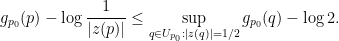
The right-hand side is finite, and this gives the required upper bound to complete the proof that ${g_{p_0}}$ has a logarithmic singularity at ${p_0}$ . This concludes the proof of Proposition 58 and hence Theorem 50.
Before we turn to the non-hyperbolic case of the uniformisation theorem, we record a symmetry property of the Green’s functions that is used to establish that case:

Proposition 64 (Symmetry of Green’s functions) Let ${M}$ be a connected Riemann surface, and suppose that the Green’s functions ${g_{p_0}: M \backslash \{p_0\} \rightarrow {\bf R}}$ exist for all ${p_0}$ . Then for all distinct ${p_0,p_1 \in M}$ , we have ${g_{p_0}(p_1) = g_{p_1}(p_0)}$ .

When ${M}$ is simply connected, this symmetry can be deduced from (7). For ${M}$ that are not simply connected, the argument is trickier, requiring one to pass to a universal cover ${N}$ of ${M}$ , establish the existence of Green’s functions on ${N}$ , and find an identity relating the Green’s functions on ${N}$ with the Green’s functions on ${M}$ . For details see Marshall’s notes.

Now we can discuss to the non-hyperbolic case of the uniformisation theorem, Theorem 51. Now we do not have any Green’s functions, or any non-constant bounded holomorphic functions. However, note that all three of the model Riemann surfaces ${D(0,1)}$ , ${{\bf C}}$ and ${{\bf C} \cup \{\infty\}}$ still have plenty of meromorphic functions: in particular, for any two distinct points ${z_0,z_1}$ in ${{\bf C}}$ , one can find a holomorphic function ${f: {\bf C} \rightarrow {\bf C} \cup \{\infty\}}$ that has a simple zero at ${z_0}$ , a simple pole at ${z_1}$ , and no other zeroes and poles, namely ${f(z) := \frac{z-z_0}{z-z_1}}$ ; one can think of this function with a zero-pole pair as a “dipole“. Similarly if one works on the domain ${{\bf C} \cup \{\infty\}}$ or ${D(0,1)}$ rather than ${{\bf C}}$ . From this we see that Theorem 51 would imply the following claim:

Theorem 65 (Existence of dipoles) Let ${M}$ be a simply connected Riemann surface. Let ${p_0,p_1}$ be distinct points in ${M}$ . Then there exists a holomorphic map ${f_{p_0,p_1}: M \rightarrow {\bf C} \cup \{\infty\}}$ that has a simple zero at ${p_0}$ , a simple pole at ${p_1}$ , and no other zeroes and poles. Furthermore, outside of a compact set ${K}$ containing ${p_0,p_1}$ , the function ${f_{p_0,p_1}}$ can be chosen to be bounded away from both ${0}$ and ${\infty}$ (that is, there exists ${C > c > 0}$ such that ${c \leq |f_{p_0,p_1}(p)| \leq C}$ for all ${p \in M \backslash K}$ ).

In the converse direction, we can use Theorem 65 to recover Theorem 51 in a manner analogous to how Theorem 52 implies Theorem 50. Indeed, let ${M}$ be a simply connected Riemann surface without non-constant holomorphic maps from ${M}$ to ${D(0,1)}$ . Given any three distinct points ${p_0,p_1,p_2}$ in ${M}$ , we consider the dipoles ${f_{p_0,p_1}}$ and ${f_{p_2,p_1}}$ . The function

$\displaystyle \frac{f_{p_0,p_1} - f_{p_0,p_1}(p_2)}{f_{p_2,p_1}} \ \ \ \ \ (9)$

has removable singularities at ${p_1}$ and at