246B, Notes 1: Zeroes, poles, and factorisation of meromorphic functions

23 December, 2020 in 246B - complex analysis, math.CV | Tags: gamma function, Hadamard factorisation theorem, Jensen's formula, Weierstrass factorisation theorem

Previous set of notes: 246A Notes 5. Next set of notes: Notes 2.

— 1. Jensen’s formula —

Suppose ${f}$ is a non-zero rational function ${f =P/Q}$ , then by the fundamental theorem of algebra one can write

$\displaystyle f(z) = c \frac{\prod_\rho (z-\rho)}{\prod_\zeta (z-\zeta)}$

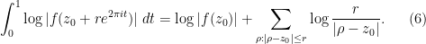
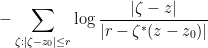
for some non-zero constant ${c}$ , where ${\rho}$ ranges over the zeroes of ${P}$ (counting multiplicity) and ${\zeta}$ ranges over the zeroes of ${Q}$ (counting multiplicity), and assuming ${z}$ avoids the zeroes of ${Q}$ . Taking absolute values and then logarithms, we arrive at the formula

$\displaystyle \log |f(z)| = \log |c| + \sum_\rho \log|z-\rho| - \sum_\zeta \log |z-\zeta|, \ \ \ \ \ (1)$

as long as ${z}$ avoids the zeroes of both ${P}$ and ${Q}$ . (In this set of notes we use ${\log}$ for the natural logarithm when applied to a positive real number, and ${\mathrm{Log}}$ for the standard branch of the complex logarithm (which extends ${\log}$ ); the multi-valued complex logarithm ${\log}$ will only be used in passing.) Alternatively, taking logarithmic derivatives, we arrive at the closely related formula

$\displaystyle \frac{f'(z)}{f(z)} = \sum_\rho \frac{1}{z-\rho} - \sum_\zeta \frac{1}{z-\zeta}, \ \ \ \ \ (2)$

again for ${z}$ avoiding the zeroes of both ${P}$ and ${Q}$ . Thus we see that the zeroes and poles of a rational function ${f}$ describe the behaviour of that rational function, as well as close relatives of that function such as the log-magnitude ${\log|f|}$ and log-derivative ${\frac{f'}{f}}$ . We have already seen these sorts of formulae arise in our treatment of the argument principle in 246A Notes 4.

Exercise 1 Let ${P(z)}$ be a complex polynomial of degree ${n \geq 1}$ .

(i) (Gauss-Lucas theorem) Show that the complex roots of ${P'(z)}$ are contained in the closed convex hull of the complex roots of ${P(z)}$ .
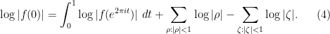
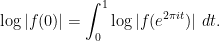
(ii) (Laguerre separation theorem) If all the complex roots of ${P(z)}$ are contained in a disk ${D(z_0,r)}$ , and ${\zeta \not \in D(z_0,r)}$ , then all the complex roots of ${nP(z) + (\zeta - z) P'(z)}$ are also contained in ${D(z_0,r)}$ . (Hint: apply a suitable Möbius transformation to move ${\zeta}$ to infinity, and then apply part (i) to a polynomial that emerges after applying this transformation.)

There are a number of useful ways to extend these formulae to more general meromorphic functions than rational functions. Firstly there is a very handy “local” variant of (1) known as Jensen’s formula:

Theorem 2 (Jensen’s formula) Let ${f}$ be a meromorphic function on an open neighbourhood of a disk ${\overline{D(z_0,r)} = \{ z: |z-z_0| \leq r \}}$ , with all removable singularities removed. Then, if ${z_0}$ is neither a zero nor a pole of ${f}$ , we have
$\displaystyle \log |f(z_0)| = \int_0^1 \log |f(z_0+re^{2\pi i t})|\ dt + \sum_{\rho: |\rho-z_0| \leq r} \log \frac{|\rho-z_0|}{r} \ \ \ \ \ (3)$

$\displaystyle - \sum_{\zeta: |\zeta-z_0| \leq r} \log \frac{|\zeta-z_0|}{r}$
where ${\rho}$ and ${\zeta}$ range over the zeroes and poles of ${f}$ respectively (counting multiplicity) in the disk ${\overline{D(z_0,r)}}$ .

One can view (3) as a truncated (or localised) variant of (1). Note also that the summands ${\log \frac{|\rho-z_0|}{r}, \log \frac{|\zeta-z_0|}{r}}$ are always non-positive.

Proof: By perturbing ${r}$ slightly if necessary, we may assume that none of the zeroes or poles of ${f}$ (which form a discrete set) lie on the boundary circle ${\{ z: |z-z_0| = r \}}$ . By translating and rescaling, we may then normalise ${z_0=0}$ and ${r=1}$ , thus our task is now to show that

$\displaystyle \log |f(0)| = \int_0^1 \log |f(e^{2\pi i t})|\ dt + \sum_{\rho: |\rho| < 1} \log |\rho| - \sum_{\zeta: |\zeta| < 1} \log |\zeta|. \ \ \ \ \ (4)$

We may remove the poles and zeroes inside the disk ${D(0,1)}$ by the useful device of Blaschke products. Suppose for instance that ${f}$ has a zero ${\rho}$ inside the disk ${D(0,1)}$ . Observe that the function

$\displaystyle B_\rho(z) := \frac{\rho - z}{1 - \overline{\rho} z} \ \ \ \ \ (5)$

has magnitude ${1}$ on the unit circle ${\{ z: |z| = 1\}}$ , equals ${\rho}$ at the origin, has a simple zero at ${\rho}$ , but has no other zeroes or poles inside the disk. Thus Jensen’s formula (4) already holds if ${f}$ is replaced by ${B_\rho}$ . To prove (4) for ${f}$ , it thus suffices to prove it for ${f/B_\rho}$ , which effectively deletes a zero ${\rho}$ inside the disk ${D(0,1)}$ from ${f}$ (and replaces it instead with its inversion ${1/\overline{\rho}}$ ). Similarly we may remove all the poles inside the disk. As a meromorphic function only has finitely many poles and zeroes inside a compact set, we may thus reduce to the case when ${f}$ has no poles or zeroes on or inside the disk ${D(0,1)}$ , at which point our goal is simply to show that

$\displaystyle \log |f(0)| = \int_0^1 \log |f(e^{2\pi i t})|\ dt.$

Since ${f}$ has no zeroes or poles inside the disk, it has a holomorphic logarithm ${F}$ (Exercise 46 of 246A Notes 4). In particular, ${\log |f|}$ is the real part of ${F}$ . The claim now follows by applying the mean value property (Exercise 17 of 246A Notes 3) to ${\log |f|}$ . $\Box$

An important special case of Jensen’s formula arises when ${f}$ is holomorphic in a neighborhood of ${\overline{D(z_0,r)}}$ , in which case there are no contributions from poles and one simply has

$\displaystyle \int_0^1 \log |f(z_0+re^{2\pi i t})|\ dt = \log |f(z_0)| + \sum_{\rho: |\rho-z_0| \leq r} \log \frac{r}{|\rho-z_0|}. \ \ \ \ \ (6)$

This is quite a useful formula, mainly because the summands ${\log \frac{r}{|\rho-z_0|}}$ are non-negative; it can be viewed as a more precise assertion of the subharmonicity of ${\log |f|}$ (see Exercises 60(ix) and 61 of 246A Notes 5). Here are some quick applications of this formula:

Exercise 3 Use (6) to give another proof of Liouville’s theorem: a bounded holomorphic function ${f}$ on the entire complex plane is necessarily constant.

Exercise 4 Use Jensen’s formula to prove the fundamental theorem of algebra: a complex polynomial ${P(z)}$ of degree ${n}$ has exactly ${n}$ complex zeroes (counting multiplicity), and can thus be factored as ${P(z) = c (z-z_1) \dots (z-z_n)}$ for some complex numbers ${c,z_1,\dots,z_n}$ with ${c \neq 0}$ . (Note that the fundamental theorem was invoked previously in this section, but only for motivational purposes, so the proof here is non-circular.)

Exercise 5 (Shifted Jensen’s formula) Let ${f}$ be a meromorphic function on an open neighbourhood of a disk ${\{ z: |z-z_0| \leq r \}}$ , with all removable singularities removed. Show that
$\displaystyle \log |f(z)| = \int_0^1 \log |f(z_0+re^{2\pi i t})| \mathrm{Re} \frac{r e^{2\pi i t} + (z-z_0)}{r e^{2\pi i t} - (z-z_0)}\ dt \ \ \ \ \ (7)$

$\displaystyle + \sum_{\rho: |\rho-z_0| \leq r} \log \frac{|\rho-z|}{|r - \rho^* (z-z_0)|}$

$\displaystyle - \sum_{\zeta: |\zeta-z_0| \leq r} \log \frac{|\zeta-z|}{|r - \zeta^* (z-z_0)|}$
for all ${z}$ in the open disk ${\{ z: |z-z_0| < r\}}$ that are not zeroes or poles of ${f}$ , where ${\rho^* = \frac{\overline{\rho-z_0}}{r}}$ and ${\zeta^* = \frac{\overline{\zeta-z_0}}{r}}$ . (The function ${\Re \frac{r e^{2\pi i t} + (z-z_0)}{r e^{2\pi i t} - (z-z_0)}}$ appearing in the integrand is sometimes known as the Poisson kernel, particularly if one normalises so that ${z_0=0}$ and ${r=1}$ .)

Exercise 6 (Bounded type)

(i) If ${f}$ is a holomorphic function on ${D(0,1)}$ that is not identically zero, show that ${\liminf_{r \rightarrow 1^-} \int_0^{2\pi} \log |f(re^{i\theta})|\ d\theta > -\infty}$ .
(ii) If ${f}$ is a meromorphic function on ${D(0,1)}$ that is the ratio of two bounded holomorphic functions that are not identically zero, show that ${\limsup_{r \rightarrow 1^-} \int_0^{2\pi} |\log |f(re^{i\theta})||\ d\theta < \infty}$ . (Functions ${f}$ of this form are said to be of bounded type and lie in the Nevanlinna class for the unit disk ${D(0,1)}$ .)

Exercise 7 (Smoothed out Jensen formula) Let ${f}$ be a meromorphic function on an open set ${U}$ , and let ${\phi: U \rightarrow {\bf C}}$ be a smooth compactly supported function. Show that
$\displaystyle \sum_\rho \phi(\rho) - \sum_\zeta \phi(\zeta)$

$\displaystyle = \frac{-1}{2\pi} \int\int_U ((\frac{\partial}{\partial x} + i \frac{\partial}{\partial y}) \phi(x+iy)) \frac{f'}{f}(x+iy)\ dx dy$

$\displaystyle = \frac{1}{2\pi} \int\int_U ((\frac{\partial^2}{\partial x^2} + \frac{\partial^2}{\partial y}^2) \phi(x+iy)) \log |f(x+iy)|\ dx dy$
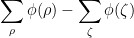
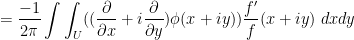
where ${\rho, \zeta}$ range over the zeroes and poles of ${f}$ (respectively) in the support of ${\phi}$ . Informally argue why this identity is consistent with Jensen’s formula.

When applied to entire functions ${f}$ , Jensen’s formula relates the order of growth of ${f}$ near infinity with the density of zeroes of ${f}$ . Here is a typical result:

Proposition 8 Let ${f: {\bf C} \rightarrow {\bf C}}$ be an entire function, not identically zero, that obeys a growth bound ${|f(z)| \leq C \exp( C|z|^\alpha)}$ for some ${C, \alpha > 0}$ and all ${z}$ . Then there exists a constant ${C'>0}$ such that ${D(0,R)}$ has at most ${C' R^\alpha}$ zeroes (counting multiplicity) for any ${R \geq 1}$ .

Entire functions that obey a growth bound of the form ${|f(z)| \leq C_\varepsilon \exp( C_\varepsilon |z|^{\rho+\varepsilon})}$ for every ${\varepsilon>0}$ and ${z}$ (where ${C_\varepsilon}$ depends on ${\varepsilon}$ ) are said to be of order at most ${\rho}$ . The above theorem shows that for such functions that are not identically zero, the number of zeroes in a disk of radius ${R}$ does not grow much faster than ${R^\rho}$ . This is often a useful preliminary upper bound on the zeroes of entire functions, as the order of an entire function tends to be relatively easy to compute in practice.

Proof: First suppose that ${f(0)}$ is non-zero. From (6) applied with ${r=2R}$ and ${z_0=0}$ one has

$\displaystyle \int_0^1 \log(C \exp( C (2R)^\alpha ) )\ dt \geq \log |f(0)| + \sum_{\rho: |\rho| \leq 2R} \log \frac{2R}{|\rho|}.$

Every zero in ${D(0,R)}$ contribute at least ${\log 2}$ to a summand on the right-hand side, while all other zeroes contribute a non-negative quantity, thus

$\displaystyle \log C + C (2R)^\alpha \geq \log |f(0)| + N_R \log 2$

where ${N_R}$ denotes the number of zeroes in ${D(0,R)}$ . This gives the claim for ${f(0) \neq 0}$ . When ${f(0)=0}$ , one can shift ${f}$ by a small amount to make ${f}$ non-zero at the origin (using the fact that zeroes of holomorphic functions not identically zero are isolated), modifying ${C}$ in the process, and then repeating the previous arguments. $\Box$

Just as (3) and (7) give truncated variants of (1), we can create truncated versions of (2). The following crude truncation is adequate for many applications:

Theorem 9 (Truncated formula for log-derivative) Let ${f}$ be a holomorphic function on an open neighbourhood of a disk ${\{ z: |z-z_0| \leq r \}}$ that is not identically zero on this disk. Suppose that one has a bound of the form ${|f(z)| \leq M^{O_{c_1,c_2}(1)} |f(z_0)|}$ for some ${M \geq 1}$ and all ${z}$ on the circle ${\{ z: |z-z_0| = r\}}$ . Let ${0 < c_2 < c_1 < 1}$ be constants. Then one has the approximate formula
$\displaystyle \frac{f'(z)}{f(z)} = \sum_{\rho: |\rho - z_0| \leq c_1 r} \frac{1}{z-\rho} + O_{c_1,c_2}( \frac{\log M}{r} )$
for all ${z}$ in the disk ${\{ z: |z-z_0| < c_2 r \}}$ other than zeroes of ${f}$ . Furthermore, the number of zeroes ${\rho}$ in the above sum is ${O_{c_1,c_2}(\log M)}$ .

Proof: To abbreviate notation, we allow all implied constants in this proof to depend on ${c_1,c_2}$ .

We mimic the proof of Jensen’s formula. Firstly, we may translate and rescale so that ${z_0=0}$ and ${r=1}$ , so we have ${|f(z)| \leq M^{O(1)} |f(0)|}$ when ${|z|=1}$ , and our main task is to show that

$\displaystyle \frac{f'(z)}{f(z)} - \sum_{\rho: |\rho| \leq c_1} \frac{1}{z-\rho} = O( \log M ) \ \ \ \ \ (8)$

for ${|z| \leq c_2}$ . Note that if ${f(0)=0}$ then ${f}$ vanishes on the unit circle and hence (by the maximum principle) vanishes identically on the disk, a contradiction, so we may assume ${f(0) \neq 0}$ . From hypothesis we then have

$\displaystyle \log |f(z)| \leq \log |f(0)| + O(\log M)$

on the unit circle, and so from Jensen’s formula (3) we see that

$\displaystyle \sum_{\rho: |\rho| \leq 1} \log \frac{1}{|\rho|} = O(\log M). \ \ \ \ \ (9)$

In particular we see that the number of zeroes with ${|\rho| \leq c_1}$ is ${O(\log M)}$ , as claimed.

Suppose ${f}$ has a zero ${\rho}$ with ${c_1 < |\rho| \leq 1}$ . If we factor ${f = B_\rho g}$ , where ${B_\rho}$ is the Blaschke product (5), then

$\displaystyle \frac{f'}{f} = \frac{B'_\rho}{B_\rho} + \frac{g'}{g}$

$\displaystyle = \frac{g'}{g} + \frac{1}{z-\rho} - \frac{1}{z-1/\overline{\rho}}.$

Observe from Taylor expansion that the distance between ${\rho}$ and ${1/\overline{\rho}}$ is ${O( \log \frac{1}{|\rho|} )}$ , and hence ${\frac{1}{z-\rho} - \frac{1}{z-1/\overline{\rho}} = O( \log \frac{1}{|\rho|} )}$ for ${|z| \leq c_2}$ . Thus we see from (9) that we may use Blaschke products to remove all the zeroes in the annulus ${c_1 < |\rho| \leq 1}$ while only affecting the left-hand side of (8) by ${O( \log M)}$ ; also, removing the Blaschke products does not affect ${|f(z)|}$ on the unit circle, and only affects ${\log |f(0)|}$ by ${O(\log M)}$ thanks to (9). Thus we may assume without loss of generality that there are no zeroes in this annulus.

Similarly, given a zero ${\rho}$ with ${|\rho| \leq c_1}$ , we have ${\frac{1}{z-1/\overline{\rho}} = O(1)}$ , so using Blaschke products to remove all of these zeroes also only affects the left-hand side of (8) by ${O(\log M)}$ (since the number of zeroes here is ${O(\log M)}$ ), with ${\log |f(0)|}$ also modified by at most ${O(\log M)}$ . Thus we may assume in fact that ${f}$ has no zeroes whatsoever within the unit disk. We may then also normalise ${f(0) = 1}$ , then ${\log |f(e^{2\pi i t})| \leq O(\log M)}$ for all ${t \in [0,1]}$ . By Jensen’s formula again, we have

$\displaystyle \int_0^1 \log |f(e^{2\pi i t})|\ dt = 0$

and thus (by using the identity ${|x| = 2 \max(x,0) - x}$ for any real ${x}$ )

$\displaystyle \int_0^1 \log |f(e^{2\pi i t})|\ dt \ll \log M. \ \ \ \ \ (10)$

On the other hand, from (7) we have

$\displaystyle \log |f(z)| = \int_0^1 \log |f(e^{2\pi i t})| \mathrm{Re} \frac{e^{2\pi i t} + z}{e^{2\pi i t} - z}\ dt$

which implies from (10) that ${\log |f(z)|}$ and its first derivatives are ${O( \log M )}$ on the disk ${\{ z: |z| \leq c_2 \}}$ . But recall from the proof of Jensen’s formula that ${\frac{f'}{f}}$ is the derivative of a logarithm ${\log f}$ of ${f}$ , whose real part is ${\log |f|}$ . By the Cauchy-Riemann equations for ${\log f}$ , we conclude that ${\frac{f'}{f} = O(\log M)}$ on the disk ${\{ z: |z| \leq c_2 \}}$ , as required. $\Box$

Exercise 10

(i) (Borel-Carathéodory theorem) If ${f: U \rightarrow {\bf C}}$ is analytic on an open neighborhood of a disk ${\overline{D(z_0,R)}}$ , show that
$\displaystyle \sup_{z \in D(z_0,r)} |f(z)| \leq \frac{2r}{R-r} \sup_{z \in \overline{D(z_0,R)}} \mathrm{Re} f(z) + \frac{R+r}{R-r} |f(z_0)|.$
(Hint: one can normalise ${z_0=0}$ , ${R=1}$ , ${f(0)=0}$ , and ${\sup_{|z-z_0| \leq R} \mathrm{Re} f(z)=1}$ . Now ${f}$ maps the unit disk to the half-plane ${\{ \mathrm{Re} z \leq 1 \}}$ . Use a Möbius transformation to map the half-plane to the unit disk and then use the Schwarz lemma.)
(ii) Use (i) to give an alternate way to conclude the proof of Theorem 9.

A variant of the above argument allows one to make precise the heuristic that holomorphic functions locally look like polynomials:

Exercise 11 (Local Weierstrass factorisation) Let the notation and hypotheses be as in Theorem 9. Then show that
$\displaystyle f(z) = P(z) \exp( g(z) )$
for all ${z}$ in the disk ${\{ z: |z-z_0| < c_2 r \}}$ , where ${P}$ is a polynomial whose zeroes are precisely the zeroes of ${f}$ in ${\{ z: |z-z_0| \leq c_1r \}}$ (counting multiplicity) and ${g}$ is a holomorphic function on ${\{ z: |z-z_0| < c_2 r \}}$ of magnitude ${O_{c_1,c_2}( \log M )}$ and first derivative ${O_{c_1,c_2}( \log M / r )}$ on this disk. Furthermore, show that the degree of ${P}$ is ${O_{c_1,c_2}(\log M)}$ .

Exercise 12 (Preliminary Beurling factorisation) Let ${H^\infty(D(0,1))}$ denote the space of bounded analytic functions ${f: D(0,1) \rightarrow {\bf C}}$ on the unit disk; this is a normed vector space with norm
$\displaystyle \|f\|_{H^\infty(D(0,1))} := \sup_{z \in D(0,1)} |f(z)|.$

(i) If ${f \in H^\infty(D(0,1))}$ is not identically zero, and ${z_n}$ denote the zeroes of ${f}$ in ${D(0,1)}$ counting multiplicity, show that
$\displaystyle \sum_n (1-|z_n|) < \infty$
and
$\displaystyle \sup_{1/2 < r < 1} \int_0^{2\pi} | \log |f(re^{i\theta})| |\ d\theta < \infty.$

(ii) Let the notation be as in (i). If we define the Blaschke product
$\displaystyle B(z) := z^m \prod_{|z_n| \neq 0} \frac{|z_n|}{z_n} \frac{z_n-z}{1-\overline{z_n} z}$
where ${m}$ is the order of vanishing of ${f}$ at zero, show that this product converges absolutely to a holomorphic function on ${D(0,1)}$ , and that ${|f(z)| \leq \|f\|_{H^\infty(D(0,1)} |B(z)|}$ for all ${z \in D(0,1)}$ . (It may be easier to work with finite Blaschke products first to obtain this bound.)
(iii) Continuing the notation from (i), establish a factorisation ${f(z) = B(z) \exp(g(z))}$ for some holomorphic function ${g: D(0,1) \rightarrow {\bf C}}$ with ${\mathrm{Re}(g(z)) \leq \log \|f\|_{H^\infty(D(0,1)}}$ for all ${z\in D(0,1)}$ .
(iv) (Theorem of F. and M. Riesz, special case) If ${f \in H^\infty(D(0,1))}$ extends continuously to the boundary ${\{e^{i\theta}: 0 \leq \theta < 2\pi\}}$ , show that the set ${\{ 0 \leq \theta < 2\pi: f(e^{i\theta})=0 \}}$ has zero measure.

Remark 13 The factorisation (iii) can be refined further, with ${g}$ being the Poisson integral of some finite measure on the unit circle. Using the Lebesgue decomposition of this finite measure into absolutely continuous parts one ends up factorising ${H^\infty(D(0,1))}$ functions into “outer functions” and “inner functions”, giving the Beurling factorisation of ${H^\infty}$ . There are also extensions to larger spaces ${H^p(D(0,1))}$ than ${H^\infty(D(0,1))}$ (which are to ${H^\infty}$ as ${L^p}$ is to ${L^\infty}$ ), known as Hardy spaces. We will not discuss this topic further here, but see for instance this text of Garnett for a treatment.

Exercise 14 (Littlewood’s lemma) Let ${f}$ be holomorphic on an open neighbourhood of a rectangle ${R = \{ \sigma+it: \sigma_0 \leq \sigma \leq \sigma_1; 0 \leq t \leq T \}}$ for some ${\sigma_0 < \sigma_1}$ and ${T>0}$ , with ${f}$ non-vanishing on the boundary of the rectangle. Show that
$\displaystyle 2\pi \sum_\rho (\mathrm{Re}(\rho)-\sigma_0) = \int_0^T \log |f(\sigma_0+it)|\ dt - \int_0^T \log |f(\sigma_1+it)|\ dt$

$\displaystyle + \int_{\sigma_0}^{\sigma_1} \mathrm{arg} f(\sigma+iT)\ d\sigma - \int_{\sigma_0}^{\sigma_1} \mathrm{arg} f(\sigma)\ d\sigma$
where ${\rho}$ ranges over the zeroes of ${f}$ inside ${R}$ (counting multiplicity) and one uses a branch of ${\mathrm{arg} f}$ which is continuous on the upper, lower, and right edges of ${C}$ . (This lemma is a popular tool to explore the zeroes of Dirichlet series such as the Riemann zeta function.)

— 2. The Weierstrass factorisation theorem —

The fundamental theorem of algebra shows that every polynomial ${P(z)}$ of degree ${n}$ comes with ${n}$ complex zeroes ${z_1,\dots,z_n}$ (counting multiplicity). In the converse direction, given any ${n}$ complex numbers ${z_1,\dots,z_n}$ (again allowing multiplicity), one can form a degree ${n}$ polynomial ${P(z)}$ with precisely these zeroes by the formula

$\displaystyle P(z) := c (z-z_1) \dots (z-z_n) \ \ \ \ \ (11)$

where ${c}$ is an arbitrary non-zero constant, and by the factor theorem this is the complete set of polynomials with this set of zeroes (counting multiplicity). Thus, except for the freedom to multiply polynomials by non-zero constants, one has a one-to-one correspondence between polynomials (excluding the zero polynomial as a degenerate case) and finite (multi-)sets of complex numbers.

As discussed earlier in this set of notes, one can think of a entire function as a sort of infinite degree analogue of a polynomial. One can then ask what the analogue of the above correspondence is for entire functions are – can one identify entire functions (not identically zero, and up to constants) by their sets of zeroes?

There are two obstructions to this. Firstly there are a number of non-trivial entire functions with no zeroes whatsoever. Most prominently, we have the exponential function ${\exp(z)}$ which has no zeroes despite being non-constant. More generally, if ${g(z)}$ is an entire function, then clearly ${\exp(g(z))}$ is an entire function with no zeroes. In particular one can multiply (or divide) any other entire function ${f(z)}$ by ${\exp(g(z))}$ without affecting the location and order of the zeroes.

Secondly, we know (see Corollary 24 of 246A Notes 3) that the set of zeroes of an entire function (that is not identically zero) must be isolated; in particular, in any compact set there can only be finitely many zeroes. Thus, by covering the complex plane by an increasing sequence of compact sets (e.g., the disks ${\overline{D(0,n)}}$ ), one can index the zeroes (counting multiplicity) by a sequence ${z_1,z_2,\dots}$ of complex numbers (possibly with repetition) that is either finite, or goes to infinity.

Now we turn to the Weierstrass factorisation theorem, which asserts that once one accounts for these two obstructions, we recover a correspondence between entire functions and sequences of zeroes.

Theorem 15 (Weierstrass factorization theorem) Let ${z_1,z_2,\dots}$ be a sequence of complex numbers that is either finite or going to infinity. Then there exists an entire function ${f}$ that has zeroes precisely at ${z_1,z_2,\dots}$ , with the order of zero of ${f}$ at each ${z_j}$ equal to the number of times ${z_j}$ appears in the sequence. Furthermore, this entire function is unique up to multiplication by exponentials of entire functions; that is to say, if ${f, \tilde f}$ are entire functions that are both of the above form, then ${\tilde f(z) = f(z) \exp(g(z))}$ for some entire function ${g}$ .

We now establish this theorem. We begin with the easier uniqueness part of the theorem. If ${\tilde f, f}$ are entire functions with the same locations and orders of zeroes, then the ratio ${\tilde f/f}$ is a meromorphic function on ${{\bf C}}$ which only has removable singularities, and becomes an entire function with no zeroes once the singularities are removed. Since the domain ${{\bf C}}$ of an entire function is simply connected, we can then take a branch of the complex logarithm ${\tilde f/f}$ (see Exercise 46 of 246A Notes 4) to write ${\tilde f/f = \exp(g)}$ for an entire function ${g}$ (after removing singularities), giving the uniqueness claim.

Now we turn to existence. If the sequence ${z_1,z_2,\dots}$ is finite, we can simply use the formula (11) to produce the required entire function ${f}$ (setting ${c}$ to equal ${1}$ , say). So now suppose that the sequence is infinite. Naively, one might try to replicate the formula (11) and set

$\displaystyle f(z) := \prod_{n=1}^\infty (z-z_n).$

Here we encounter a serious problem: the infinite product ${\prod_{n=1}^\infty (z-z_n)}$ is likely to be divergent (that is to say, the partial products ${\prod_{n=1}^N (z-z_n)}$ ) fail to converge, given that the factors ${z-z_n}$ go off to infinity. On the other hand, we do have this freedom to multiply ${f}$ by a constant (or more generally, the exponential of an entire function). One can try to use this freedom to “renormalise” the factors ${z-z_n}$ to make them more likely to converge. Much as an infinite series ${\sum_{n=1}^\infty a_n}$ is more likely to converge when its summands ${a_n}$ converge rapidly to zero, an infinite series ${\prod_{n=1}^\infty a_n}$ is more likely to converge when its factors ${a_n}$ converge rapidly to ${1}$ . Here is one formalisation of this principle:

Lemma 16 (Absolutely convergent products) Let ${a_n}$ be a sequence of complex numbers such that ${\sum_{n=1}^\infty |a_n-1| < \infty}$ . Then the product ${\prod_{n=1}^\infty a_n}$ converges. Furthermore, this product vanishes if and only if one of the factors ${a_n}$ vanishes.

Products covered by this lemma are known as absolutely convergent products. It is possible for products to converge without being absolutely convergent, but such “conditionally convergent products” are infrequently used in mathematics.

Proof: By the zero test, ${|a_n-1| \rightarrow 0}$ , thus ${a_n}$ converges to ${1}$ . In particular, all but finitely many of the ${a_n}$ lie in the disk ${D(1,1/2)}$ . We can then factor ${\prod_{n=1}^\infty a_n = \prod_{n=1}^N a_n \times \prod_{n=N+1}^\infty a_n}$ , where ${N}$ is such that ${a_n \in D(1,1/2)}$ for ${n > N}$ , and we see that it will suffice to show that the infinite product ${\prod_{n=N+1}^\infty a_n}$ converges to a non-zero number. But on using the standard branch ${\mathrm{Log}}$ of the complex logarithm on ${D(1,1/2)}$ we can write ${a_n = \exp( \mathrm{Log} a_n )}$ . By Taylor expansion we have ${\mathrm{Log} a_n = O( |a_n-1| )}$ , hence the series ${\sum_{n=N+1}^\infty \mathrm{Log} a_n}$ is absolutely convergent. From the properties of the complex exponential we then see that the product ${\prod_{n=N+1}^\infty a_n}$ converges to ${\exp(\sum_{n=N+1}^\infty \mathrm{Log} a_n)}$ , giving the claim. $\Box$

It is well known that absolutely convergent series are preserved by rearrangement, and the same is true for absolutely convergent products:

Exercise 17 If ${\prod_{n=1}^\infty a_n}$ is an absolutely convergent product of complex numbers ${a_n}$ , show that any permutation of the ${a_n}$ leads to the same absolutely convergent product, thus ${\prod_{n=1}^\infty a_n = \prod_{m=1}^\infty a_{\phi(m)}}$ for any permutation ${\phi}$ of the positive integers ${\{1,2,3,\dots\}}$ .

Exercise 18

(i) Let ${a_n}$ be a sequence of real numbers with ${a_n \geq 1}$ for all ${n}$ . Show that ${\prod_{n=1}^\infty a_n}$ converges if and only if ${\sum_{n=1}^\infty (a_n-1)}$ converges.
(ii) Let ${z_n}$ be a sequence of complex numbers. Show that ${\prod_{n=1}^\infty (1+z_n)}$ is absolutely convergent if and only if ${\prod_{n=1}^\infty (1+|z_n|)}$ is convergent.

To try to use Lemma 16, we can divide each factor ${z-z_n}$ by the constant ${-z_n}$ to make it closer to ${1}$ in the limit ${n \rightarrow \infty}$ . Since

$\displaystyle \frac{z-z_n}{-z_n} = 1 - \frac{z}{z_n}$

we can thus attempt to construct the desired entire function ${f}$ using the formula

$\displaystyle f(z) = \prod_{n=1}^\infty (1 - \frac{z}{z_n}). \ \ \ \ \ (12)$

Immediately there is the objection that this product is undefined if one or more of the putative zeroes ${z_n}$ is located at the origin, this objection is easily dealt with since the origin can only occur finitely many (say ${m}$ ) times, so if we remove the ${m}$ copies of the origin from the sequence of zeroes ${z_n}$ , apply the Weierstrass factorisation theorem to the remaining zeroes, and then multiply the resulting entire function by ${z^m}$ , we can reduce to the case where the origin is not one of the zeroes.

In order to apply Lemma 16 to make this product converge, we would need ${\sum_{n=1}^\infty \frac{|z|}{|z_n|}}$ to converge for every ${z}$ , or equivalently that

$\displaystyle \sum_{n=1}^\infty \frac{1}{|z_n|} < \infty. \ \ \ \ \ (13)$

This is basically a requirement that the ${z_n}$ converge to infinity sufficiently quickly. Not all sequences ${z_n}$ covered by Theorem 15 obey this condition, but let us begin with this case for sake of argument. Lemma 16 now tells us that ${f(z)}$ is well-defined for every ${z}$ , and vanishes if and only if ${z}$ is equal to one of the ${z_n}$ . However, we need to establish holomorphicity. This can be accomplished by the following product form of the Weierstrass ${M}$ -test.

Exercise 19 (Product Weierstrass ${M}$ -test) Let ${X}$ be a set, and for any natural number ${n}$ , let ${f_n: X \rightarrow {\bf C}}$ be a bounded function. If the sum ${\sum_{n=1}^\infty \sup_{x \in X} |f_n(x)-1| \leq M}$ for some finite ${M}$ , show that the products ${\prod_{n=1}^N f_n}$ converge uniformly to ${\prod_{n=1}^\infty f_n}$ on ${X}$ . (In particular, if ${X}$ is a topological space and all the ${f_n}$ are continuous, then ${\prod_{n=1}^\infty f_n}$ is continuous also.)

Using this exercise, we see that (under the assumption (13)) that the partial products ${\prod_{n=1}^N (1 - \frac{z}{z_n})}$ converge locally uniformly to the infinite product in (12). Since each of the partial products are entire, and the (locally) uniform limit of holomorphic functions is holomorphic (Theorem 34 of 246A Notes 3), we conclude that the function (12) is entire. Finally, if a certain zero ${z_j}$ appears ${m}$ times in the sequence, then after factoring out ${m}$ copies of ${(1-\frac{z}{z_j})}$ we see that ${f(z)}$ is the product of ${(1-\frac{z}{z_j})^m}$ with an entire function that is non-vanishing at ${z_j}$ , and thus ${f}$ has a zero of order exactly ${m}$ at ${z_j}$ . This establishes the Weierstrass approximation theorem under the additional hypothesis that (13) holds.

What if (13) does not hold? The problem now is that our renormalized factors ${1 - \frac{z}{z_n}}$ do not converge fast enough for Lemma 16 or Exercise 19 to apply. So we need to renormalize further, taking advantage of our ability to not just multiply by constants, but also by exponentials of entire functions. Observe that if ${z}$ is fixed and ${n}$ is large enough, then ${1 - \frac{z}{z_n}}$ lies in ${D(1,1/2)}$ and we can write

$\displaystyle 1 - \frac{z}{z_n} = \exp( \mathrm{Log}( 1 - \frac{z}{z_n} ) ).$

The function ${\mathrm{Log}( 1 - \frac{z}{z_n} )}$ is not entire, but its Taylor approximation ${-\frac{z}{z_n}}$ is. So it is natural to split

$\displaystyle 1 - \frac{z}{z_n} = \exp(-\frac{z}{z_n}) \exp( \mathrm{Log}( 1 - \frac{z}{z_n} ) + \frac{z}{z_n} ) = \exp(-\frac{z}{z_n}) e^{\frac{z}{z_n}} (1-\frac{z}{z_n}).$

We now discard the ${\exp(-\frac{z}{z_n})}$ factors (which do not affect the zeroes) and now propose the new candidate entire function

$\displaystyle f(z) = \prod_{n=1}^\infty e^{\frac{z}{z_n}} (1-\frac{z}{z_n}).$

The point here is that for ${n}$ large enough, Taylor expansion gives

$\displaystyle \mathrm{Log}( 1 - \frac{z}{z_n} ) + \frac{z}{z_n} = O( \frac{|z|^2}{|z_n|^2})$

and thus on exponentiating

$\displaystyle e^{\frac{z}{z_n}} (1-\frac{z}{z_n}) = 1 + O( \frac{|z|^2}{|z_n|^2}).$

Repeating the previous arguments, we can then verify that ${f}$ is an entire function with the required properties as long as we have the hypothesis

$\displaystyle \sum_{n=1}^\infty \frac{1}{|z_n|^2} < \infty \ \ \ \ \ (14)$

which is weaker than (13) (for instance it is obeyed when ${z_n=n}$ , whereas (13) fails in this case).

This suggests the way forward to the general case of the Weierstrass factorisation theorem, by using increasingly accurate Taylor expansions of

$\displaystyle \mathrm{Log}( 1 - \frac{z}{z_n} ) = -\frac{z}{z_n}-\frac{1}{2} \frac{z^2}{z_n^2} - \frac{1}{3} \frac{z^3}{z_n^3} - \dots$

when ${|z|/|z_n| \leq 1/2}$ . To formalise this strategy, it is convenient to introduce the canonical factors

$\displaystyle E_k(z) := (1-z) \exp( \sum_{j=1}^k \frac{z^j}{j} ) \ \ \ \ \ (15)$

for any complex number ${z}$ and natural number ${k}$ , thus

$\displaystyle E_0(z) = 1-z; \quad E_1(z) = e^z (1-z); \quad E_2(z) = e^{z+z^2/2} (1-z).$

For any fixed ${k}$ , these functions are entire and have precisely one zero, at ${z=1}$ . In the disk ${D(0,1/2)}$ , the Taylor expansion

$\displaystyle \mathrm{Log}(1-z) = - z - \frac{z^2}{2} - \frac{z^3}{3} - \dots$

indicates that the ${E_k(z)}$ converge uniformly to ${1}$ as ${k \rightarrow \infty}$ . Indeed, for ${z \in D(0,1/2)}$ we have

$\displaystyle E_k(z) = \exp( - \sum_{j=k+1}^\infty \frac{z^j}{j} )$

$\displaystyle = \exp( \sum_{j=k+1}^\infty O( 2^{-j}/k ) )$

$\displaystyle = \exp( O( 2^{-k} ) )$

$\displaystyle = 1 + O(2^{-k}) \ \ \ \ \ (16)$

For our choice of entire function ${f}$ we can now try

$\displaystyle f(z) := \prod_{n=1}^\infty E_{k_n}(z/z_n)$

where ${k_1,k_2,\dots}$ are natural numbers we are at liberty to choose. To get as good a convergence for the product we can make the ${k_n}$ go to infinity as fast as we please; but it turns out that the (somewhat arbitrary) choice of ${k_n := n}$ will suffice for proving Weierstrass’s theorem, that is to say the product

$\displaystyle f(z) := \prod_{n=1}^\infty E_n(z/z_n)$

is absolutely convergent (so that Lemma 16 and Exercise 19 applies, producing an entire function with the required zeroes). Indeed, for ${z}$ in any disk ${D(0,R)}$ , there is some ${n_0}$ such that ${|z_n| \geq 2R}$ for ${n \geq n_0}$ , and for such ${n}$ we have ${E_n(z/z_n)-1 = O( 2^{-n})}$ by (16), giving the desired uniform absolute convergence on any disk ${D(0,R)}$ , establishing the Weierstrass theorem.

Exercise 20 Let ${U}$ be a connected non-empty open subset of ${{\bf C}}$ .

(i) Show that if ${z_1,z_2,\dots}$ is any sequence of points in ${U}$ , that has no accumulation point inside ${U}$ , then there exists a holomorphic function ${f: U \rightarrow {\bf C}}$ that has zeroes precisely at the ${z_j}$ , with the order of each zero ${z_j}$ being the number of times ${z_j}$ occurs in the sequence.
(ii) Show that any meromorphic function on ${U}$ can be expressed as the ratio of two holomorphic functions on ${U}$ (with the denominator being non-zero). Conclude that the field of meromorphic functions on ${U}$ is the fraction field of the ring of holomorphic functions on ${U}$ .

Exercise 21 (Mittag-Leffler theorem, special case) Let ${z_n}$ be a sequence of distinct complex numbers going to infinity, and for each ${n}$ , let ${P_n}$ be a polynomial. Show that there exists a meromorphic function ${f: {\bf C} \backslash \{z_1,z_2,\dots\} \rightarrow {\bf C}}$ whose singularity at each each ${z_n}$ is given by ${P_n(\frac{1}{z-z_n})}$ , in the sense that ${f(z) - P_n(\frac{1}{z-z_n})}$ has a removable singularity at ${z_n}$ . (Hint: consider a sum of the form ${\sum_n P_n(\frac{1}{z-z_n}) - Q_n(z)}$ , where ${Q_n(z)}$ is a partial Taylor expansion of ${P_n(\frac{1}{z-z_n})}$ in the disk ${D(0,|z_n|/2)}$ , chosen so that the sum becomes locally uniformly absolutely convergent.) This is a special case of the Mittag-Leffler theorem, which is the same statement but in which the domain ${{\bf C}}$ is replaced by an arbitrary open set ${U}$ ; however, the proof of this generalisation is more difficult, requiring tools such as Runge’s approximation theorem which are not covered here.

— 3. The Hadamard factorisation theorem —

The Weierstrass factorisation theorem (and its proof) shows that any entire function ${f}$ that is not identically zero can be factorised as

$\displaystyle f(z) = e^{g(z)} z^m \prod_n E_n(z/z_n)$

where ${m}$ is the order of vanishing of ${f}$ at the origin, ${z_n}$ are the zeroes of ${f}$ away from the origin (counting multiplicity), and ${g}$ is an additional entire function. However, this factorisation is not always convenient to work with in practice, in large part because the index ${n}$ of the canonical factors ${E_n}$ involved are unbounded, and also because not much information is provided about the entire function ${g}$ . It turns out the situation becomes better if the entire function ${f}$ is also known to be of order at most ${\rho}$ for some ${\rho \geq 0}$ , by which we mean that

$\displaystyle |f(z)| \leq C_\varepsilon \exp( |z|^{\rho+\varepsilon})$

for every ${\varepsilon>0}$ and ${z}$ , or in asymptotic notation

$\displaystyle f(z) = O_\varepsilon(\exp( |z|^{\rho+\varepsilon} )). \ \ \ \ \ (17)$

In this case we expect to obtain a more precise factorisation for the following reason. Let us suppose we are in the simplest case where ${f}$ has no zeroes whatsoever. Then we have ${f = \exp(g)}$ for an entire function ${g}$ . From (17) we then have

$\displaystyle \mathrm{Re} g(z) \leq O_\varepsilon(( 1 + |z|)^{\rho+\varepsilon}) \ \ \ \ \ (18)$

for all ${z}$ . This only controls the real part of ${g}$ from above, but by applying the Borel-Carathéodory theorem (Exercise 10) to the disks ${\overline{D(0,2|z|)}}$ we obtain a bound of the form

$\displaystyle g(z) = O_{\rho,\varepsilon,g(0)}( (1 + |z|)^{\rho+\varepsilon} )$

for all ${\varepsilon>0}$ and all ${z}$ . That is to say, ${g}$ is of polynomial growth of order at most ${\rho}$ . Applying Exercise 31 of 246A Notes 3, we conclude that ${g}$ must be a polynomial, and given its growth rate, it must have degree at most ${d}$ , where ${d := \lfloor \rho \rfloor}$ is the integer part of ${\rho}$ . This hints that the entire function ${g}$ that appears in the Weierstrass factorisation theorem could be taken to be a polynomial, if the theorem is formulated correctly. This is indeed the case, and is the content of the Hadamard factorisation theorem:

Theorem 22 (Hadamard factorisation theorem) Let ${\rho \geq 0}$ , let ${d := \lfloor \rho \rfloor}$ , and let ${f}$ be an entire function of order at most ${\rho}$ (not identically zero), with a zero of order ${m \geq 0}$ at the origin and the remaining zeroes indexed (with multiplicity) as a finite or infinite sequence ${z_1, z_2, \dots}$ . Then
$\displaystyle f(z) = e^{g(z)} z^m \prod_n E_d(z/z_n) \ \ \ \ \ (19)$
for some polynomial ${g}$ of degree at most ${d}$ . The convergence in the infinite product is locally uniform.

We now prove this theorem. By dividing out by ${z^m}$ (which does not affect the order of ${f}$ ) and removing the singularity at the origin, we may assume that ${m=0}$ . If there are no other zeroes ${z_n}$ then we are already done by the previous discussion; similarly if there are only finitely many zeroes ${z_n}$ we can divide out by the finite number of elementary factors and remove singularities and again reduce to a case we have already established. Hence we may suppose that the sequence of zeroes ${z_n}$ is infinite. As the zeroes of ${f}$ are isolated, this forces ${z_n}$ to go to infinity as ${n \rightarrow \infty}$ .

Let us first check that the product ${\prod_{n=1}^\infty E_d(z/z_n)}$ is absolutely convergent and locally uniform. A modification of the bound (16) shows that

$\displaystyle E_d(z/z_n) = 1 + O_d( |z|^{d+1}/|z_n|^{d+1})$

if ${|z|/|z_n| \leq 1/2}$ , which is the case for all but finitely many ${n}$ if ${z}$ is confined to a fixed compact set. Thus we will get absolute convergence from Lemma 16 (and also holomorphicity of the product from Exercise 19) once we establish the convergence

$\displaystyle \sum_{n=1}^\infty \frac{1}{|z_n|^{d+1}} < \infty \ \ \ \ \ (20)$

(compare with (13), (14), which are basically the ${d=0,1}$ cases of this analysis).

To achieve this convergence we will use the technique of dyadic decomposition (a generalisation of the Cauchy condensation test). Only a finite number of zeroes ${z_n}$ lie in the disk ${D(0,1)}$ , and we have already removed all zeroes at the origin, so by removing those finite zeroes we may assume that ${|z_n| \geq 1}$ for all ${n}$ . In particular, each remaining zero ${z_n}$ lies in an annulus ${\{ z: 2^k \leq |z| < 2^{k+1}\}}$ for some natural number ${k}$ . On each such annulus, the expression ${\frac{1}{|z_n|^{d+1}}}$ is at most ${2^{-k(d+1)}}$ (and is in fact comparable to this quantity up to a constant depending on ${d}$ , which is why we expect the dyadic decomposition method to be fairly efficient). Grouping the terms in (20) according to the annulus they lie in, it thus suffices to show that

$\displaystyle \sum_{k=0}^\infty \frac{N_k}{2^{k(d+1)}} < \infty$

where ${N_k}$ is the number of zeroes of ${f}$ (counting multiplicity) in the annulus ${\{ z: 2^k \leq |z| < 2^{k+1}\}}$ . But by Proposition 8, one has ${N_k = O_{\rho,\varepsilon,f}( 2^{k(\rho+\varepsilon)})}$ for any ${\varepsilon>0}$ . Since ${d}$ is the integer part of ${\rho}$ , one can choose ${\varepsilon}$ small enough that ${\rho+\varepsilon < d+1}$ , and so the series is dominated by a convergent geometric series and is thus itself convergent. This establishes the convergence of the product ${\prod_n E_d(z/z_n)}$ . This function has zeroes in the same locations as ${f}$ with the same orders, so by the same arguments as before we have

$\displaystyle f(z) = e^{g(z)} \prod_{n=1}^\infty E_d(z/z_n)$

for some entire function ${g}$ . It remains to show that ${g}$ is a polynomial of degree at most ${d}$ . If we could show the bound (18) for all ${z}$ and any ${\varepsilon>0}$ , we would be done. Taking absolute values and logarithms, we have

$\displaystyle \mathrm{Re} g(z) = \log |f(z)| - \sum_{n=1}^\infty \log |E_d(z/z_n)|$

for ${z \neq z_1,z_2,\dots}$ and hence as ${f}$ is of order ${\rho}$ , we have

$\displaystyle \mathrm{Re} g(z) \leq O_{f,\rho,\varepsilon}( (1+|z|)^{\rho+\varepsilon} ) - \sum_{n=1}^\infty \log |E_d(z/z_n)|$

for ${z \neq z_1,z_2,\dots}$ . So if, for a given choice of ${\varepsilon>0}$ , we could show the lower bound

$\displaystyle \sum_{n=1}^\infty \log |E_d(z/z_n)| \geq - O_{f,\rho,\varepsilon}( (1+|z|)^{\rho+\varepsilon} ) \ \ \ \ \ (21)$

for all ${z \neq z_1,z_2,\dots}$ , we would be done (since ${g}$ is continuous at each ${z_n}$ , so the restriction ${z \neq z_1,z_2,\dots}$ can be removed as far as upper bounding ${g}$ is concerned). Unfortunately this can’t quite work as stated, because the factors ${E_d(z/z_n)}$ go to zero as ${z}$ approaches ${z_n}$ , so ${\log |E_d(z/z_n)|}$ approaches ${-\infty}$ . So the desired bound (21) can’t work when ${z}$ gets too close to one of the zeroes ${z_n}$ . On the other hand, this logarithmic divergence is rather mild, so one can hope to somehow evade it. Indeed, suppose we are still able to obtain (21) for a sufficiently “dense” set of ${z}$ , and more precisely for all ${z}$ on a sequence ${\{ |z| = R_k \}}$ of circles of radii ${2^k \leq R_k <2^{k+1}}$ for ${k=1,2,\dots}$ . Then the above argument lets us establish the upper bound

$\displaystyle \mathrm{Re} g(z) \leq O_{f,\rho,\varepsilon}( (1+|z|)^{\rho+\varepsilon} )$

when ${|z|=R_k}$ . But by the maximum principle (applied to the harmonic function ${\mathrm{Re} g}$ ) this then gives

$\displaystyle \mathrm{Re} g(z) \leq O_{f,\rho,\varepsilon}( (1+|z|)^{\rho+\varepsilon} )$

for all ${z}$ (because we have an upper bound of ${O_{f,\rho,\varepsilon}( (1+R_k)^{\rho+\varepsilon} )}$ on each disk ${D(0,R_k)}$ , and each ${z}$ lies in one of the disks ${D(0,R_k)}$ with ${1+|z| \sim 1+R_k}$ ).

So it remains to establish (21) for ${z}$ in a sufficiently dense set of circles ${\{ |z| = R_k\}}$ . We need lower bounds on ${\log |E_d(z/z_n)|}$ . In the regime where the zeroes are distant in the sense that ${|z|/|z_n| \leq 1/2}$ , Taylor expansion gives

$\displaystyle E_d(z/z_n) = \exp( O_d( |z|^{d+1}/|z_n|^{d+1} ) )$

and hence

$\displaystyle \sum_{n: |z|/|z_n| \leq 1/2} \log |E_d(z/z_n)| \geq - O_d( \sum_{n: |z|/|z_n| \leq 1/2} |z|^{d+1}/|z_n|^{d+1} ).$

We can adapt the proof of (20) to control this portion adequately:

Exercise 23 Establish the upper bounds
$\displaystyle \sum_{n: |z|/|z_n| \leq 1/2} |z|^{d+1}/|z_n|^{d+1} \leq O_{f,\rho,\varepsilon}( (1+|z|)^{\rho+\varepsilon} )$
and
$\displaystyle \sum_{n: |z|/|z_n| > 1/2} |z|^{d}/|z_n|^{d} \leq O_{f,\rho,\varepsilon}( (1+|z|)^{\rho+\varepsilon} )$
(the latter bound will be useful momentarily).

It thus remains to control the nearby zeroes, in the sense of showing that

$\displaystyle \sum_{n: |z|/|z_n| > 1/2} \log |E_d(z/z_n)| \geq -O_{f,\rho,\varepsilon}( (1+|z|)^{\rho+\varepsilon} )$

for all ${z}$ in a set of concentric circles ${\{ |z| = R_k\}}$ with ${2^k \leq R_k < 2^{k+1}}$ . Thus we need to lower bound ${\log |E_d(w)|}$ for ${|w| > 1/2}$ . Here we no longer attempt to take advantage of Taylor expansion as the convergence is too poor in this regime, so we fall back to the triangle inequality. Indeed from (15) and that inequality we have

$\displaystyle \log |E_d(w)| \geq - \log \frac{1}{|1-w|} - \sum_{j=1}^d \frac{|w|^j}{j} \geq -\log \frac{1}{|1-w|} - O_d(|w|^d)$

hence

$\displaystyle \sum_{n: |z|/|z_n| > 1/2} \log |E_d(z/z_n)| \geq -\sum_{n: |z|/|z_n| > 1/2} \log \frac{1}{|1-z/z_n|}$

$\displaystyle - O_d(\sum_{n: |z|/|z_n| > 1/2} \frac{|z|^d}{|z_n|^d} ).$

From the second part of Exercise 23, the contribution of the latter term is acceptable, so it remains to establish the upper bound

$\displaystyle \sum_{n: |z|/|z_n| > 1/2} \log \frac{1}{|1-z/z_n|} \leq O_{f,\rho,\varepsilon}( (1+|z|)^{\rho+\varepsilon} )$

for ${z}$ in a set of concentric circles ${\{ |z| = R_k\}}$ with ${2^k \leq R_k < 2^{k+1}}$ .

Given the set of ${z}$ we are working with, it is natural to introduce the radial variable ${r := |z|}$ . From the triangle inequality one has ${|1-z/z_n| \geq |1-r/|z_n||}$ , so it will suffice to show that

$\displaystyle \sum_{n: r/|z_n| > 1/2} \log \frac{1}{|1-r/|z_n||} \leq O_{f,\rho,\varepsilon}( 2^{(\rho+\varepsilon)k} )$

for at least one radius ${r \in [2^k, 2^{k+1})}$ for each natural number ${k}$ . Note that we cannot just pick any radius ${r}$ here, because if ${r}$ happens to be too close to one of the ${|z_n|}$ then the term ${\log \frac{1}{|1-r/|z_n||}}$ will become unbounded. But we can avoid this by the strategy of the probabilistic method: we just choose ${r}$ randomly in the interval ${[2^k, 2^{k+1})}$ . As long we can establish the average bound

$\displaystyle \frac{1}{2^k} \int_{2^k}^{2^{k+1}} \sum_{n: r/|z_n| > 1/2} \log \frac{1}{|1-r/|z_n||}\ dr \leq O_{f,\rho,\varepsilon}( 2^{(\rho+\varepsilon)k} )$

we can use the pigeonhole principle to find one good radius ${r}$ in the desired range, which is all we need.

The point is that this averaging can take advantage of the mild nature of the logarithmic singularity. Indeed a routine computation shows that

$\displaystyle \frac{1}{2^k} \int_{2^k}^{2^{k+1}} 1_{r/R > 1/2} \log \frac{1}{|1-r/R|}\ dr$

vanishes unless ${R \leq 2^{k+2}}$ and is bounded by ${O(1)}$ otherwise, so by the linearity of integration and the triangle inequality the left-hand side is bounded by

$\displaystyle O( \sum_{n: |z_n| \leq 2^{k+2}} 1 )$

and the claim now follows from Proposition 8. This concludes the proof of the Hadamard factorisation theorem.

Exercise 24 (Converse to Hadamard factorisation) Let ${\rho \geq 0}$ , let ${m}$ be a natural number, and let ${z_1,z_2,\dots}$ be a finite or infinite sequence of non-zero complex numbers such that ${\sum_{n=1}^\infty \frac{1}{|z_n|^{\rho+\varepsilon}} < \infty}$ for every ${\varepsilon>0}$ . Let ${d := \lfloor \rho\rfloor}$ . Show that for every polynomial ${g}$ of degree at most ${d}$ , the function ${f}$ defined by (19) is an entire function of order at most ${\rho}$ , with a zero of order ${m}$ at the origin, zeroes at each ${z_j}$ of order equal to the number of times ${z_j}$ occurs in the sequence, and no other zeroes. Thus we see that we have a one-to-one correspondence between non-trivial entire functions of order at most ${\rho}$ ( up to multiplication by ${e^{g(z)}}$ factors for ${g}$ a polynomial of degree at most ${d}$ ) and zeroes ${z_n}$ obeying a certain growth condition.

As an illustration of the Hadamard factorisation theorem, we apply it to the entire function ${\sin(z)}$ . Since

$\displaystyle \sin(z) = O( |e^{iz}| + |e^{-iz}| ) = O( \exp( |z| ) )$

we see that ${\sin}$ is of order at most ${1}$ (indeed it is not difficult to show that its order is exactly ${1}$ ). Also, its zeroes are the integer multiples ${\pi n}$ of ${\pi}$ , with ${n \in {\bf Z}}$ . The Hadamard factorisation theorem then tells us that we have the product expansion

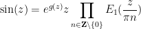$\displaystyle \sin(z) = e^{g(z)} z \prod_{n \in {\bf Z} \backslash \{0\}} E_1(\frac{z}{\pi n})$

for some polynomial ${g}$ of degree at most ${1}$ . Writing ${E_1(\frac{z}{\pi n}) = e^{z/\pi n} (1 - \frac{z}{\pi n})}$ we can group together the ${n}$ and ${-n}$ terms in the absolutely convergent product to get

$\displaystyle E_1(\frac{z}{\pi n}) E_1(\frac{z}{\pi (-n)}) = (1 - \frac{z^2}{\pi^2 n^2})$

so the Hadamard factorisation can also be written in the form

$\displaystyle \sin(z) = e^{g(z)} z \prod_{n=1}^\infty (1 - \frac{z^2}{\pi^2 n^2}).$

But what is ${g(z)}$ ? Dividing by ${z}$ and taking a suitable branch ${\tilde \log}$ of the logarithm of ${\frac{\sin z}{z}}$ we see that

$\displaystyle \tilde \log \frac{\sin z}{z} = g(z) + \sum_{n=1}^\infty \mathrm{Log} (1 - \frac{z^2}{\pi^2 n^2}) \ \ \ \ \ (22)$

for ${z}$ sufficiently close to zero (removing the singularity of ${\frac{\sin z}{z}}$ at the origin). By Taylor expansion we have

$\displaystyle \frac{\sin z}{z} = 1 - \frac{z^2}{3!} + \dots$

and

$\displaystyle \mathrm{Log} (1 - \frac{z^2}{\pi^2 n^2}) = - \frac{z^2}{\pi^2 n^2} + \dots$

for ${z}$ close to ${1}$ , thus

$\displaystyle \tilde \log \frac{\sin z}{z} = 2k \pi i - \frac{z^2}{3!} + \dots$

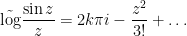for some integer ${k}$ . Since ${g}$ is linear, we conclude on comparing coefficients that ${g}$ must in fact just be a constant ${2k \pi i}$ , and we can in fact normalise ${k=0}$ since shifting ${g}$ by an integer multiple of ${2\pi i}$ does not affect ${e^{g(z)}}$ . We conclude the Euler sine product formula

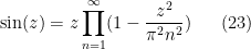
$\displaystyle \sin(z) = z \prod_{n=1}^\infty (1 - \frac{z^2}{\pi^2 n^2}) \ \ \ \ \ (23)$

(first conjectured by Euler in 1734). Inspecting the ${z^2}$ coefficients of (22), we also see that

$\displaystyle -\frac{1}{3!} = \sum_{n=1}^\infty -\frac{1}{\pi^2 n^2}$

which rearranges to yield Euler’s famous formula

$\displaystyle \sum_{n=1}^\infty \frac{1}{n^2} = \frac{\pi^2}{6} \ \ \ \ \ (24)$

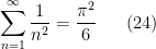
that solves the Basel problem. Observe that by inspecting higher coefficients ${z^{2k}}$ of the Taylor series one more generally obtains identities of the form

$\displaystyle \sum_{n=1}^\infty \frac{1}{n^{2k}} = b_{2k} \pi^{2k}$

for all positive integers ${k}$ and some rational numbers ${b_{2k}}$ (which are essentially Bernoulli numbers). Applying (23) to ${z=\pi/2}$ and rearranging one also gets the famous Wallis product

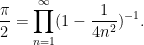
$\displaystyle \frac{\pi}{2} = \prod_{n=1}^\infty (1 - \frac{1}{4n^2})^{-1}.$

Hadamard’s theorem also tells us that any other entire function of order at most ${1}$ that has simple zeroes at the integer multiples of ${\pi}$ , and no other zeroes, must take the form ${e^{az+b} \sin(z)}$ for some complex numbers ${a,b}$ . Thus the sine function is almost completely determined by its set of zeroes, together with the fact that it is an entire function of order ${1}$ .

Exercise 25 Show that
$\displaystyle \sum_{n \in {\bf Z}} \frac{1}{z^2 - n^2} = \frac{\pi \cot(\pi z)}{z}$
for any complex number ${z}$ that is not an integer. Use this to give an alternate proof of (24).

— 4. The Gamma function —

As we saw in the previous section (and after applying a simple change of variables), the only entire functions of order ${1}$ that have simple zeroes at the integers (and nowhere else) are of the form ${e^{az+b} \sin(\pi z)}$ . It is natural to ask what happens if one replaces the integers by the natural numbers ${\{0, 1, 2, \dots\}}$ ; one could think of such functions as being in some sense “half” of the function ${\sin(\pi z)}$ . Actually, it is traditional to normalise the problem a different way, and ask what entire functions of order ${1}$ have zeroes at the non-positive integers ${0, -1, -2, -3, \dots}$ ; it is also traditional to refer to the complex variable in this problem by ${s}$ instead of ${z}$ . By the Hadamard factorisation theorem, such functions must take the form

$\displaystyle f(s) = s e^{as+b} \prod_{n=1}^\infty E_1(-s/n)$

$\displaystyle =s e^{as+b} \prod_{n=1}^\infty e^{-s/n} (1+\frac{s}{n})$

for some complex numbers ${a,b}$ ; conversely, Exercise 24 tells us that every function of this form is entire of order at most ${1}$ , with simple zeroes at ${0,-1,-2,\dots}$ . We are free to select the constants ${a,b}$ as we please to produce a function ${f}$ of this class. It is traditional to normalise ${b=0}$ ; for the most natural normalisation of ${a}$ , see below.

What properties would such functions have? The zero set ${0,-1,-2,\dots}$ are nearly invariant with respect to the shift ${s \mapsto s+1}$ , so one expects ${f(s)}$ and ${f(s+1)}$ to be related. Indeed we have

$\displaystyle f(s+1) = (s+1) e^{as+a} \prod_{n=1}^\infty e^{-(s+1)/n} (1+\frac{s+1}{n})$

$\displaystyle = (s+1) e^{as+a} \prod_{n=2}^\infty e^{-(s+1)/(n-1)} (1+\frac{s+1}{n-1})$

$\displaystyle = (s+1) e^{as+a} \prod_{n=2}^\infty e^{-s/(n-1)} (1+\frac{s}{n}) (1+\frac{1}{n-1}) e^{-1/(n-1)}$

while

$\displaystyle f(s) = s e^{as} e^{-s} (1+s) \prod_{n=2}^\infty e^{-s/n} (1+\frac{s}{n})$

so we have (using the telescoping series ${\sum_{n=2}^\infty \frac{1}{n-1}-\frac{1}{n} = 1}$ )

$\displaystyle s f(s+1) = f(s) e^a \prod_{n=2}^\infty (1+\frac{1}{n-1}) e^{-1/(n-1)}$

$\displaystyle = f(s) e^a \prod_{n=1}^\infty (1+\frac{1}{n}) e^{-1/n}.$

It is then natural to normalise ${a}$ to be the real number ${\gamma}$ for which

$\displaystyle e^\gamma \prod_{n=1}^\infty (1+\frac{1}{n}) e^{-1/n} = 1.$

This number is known as the Euler-Mascheroni constant and is approximately equal to ${0.577\dots}$ . Taking logarithms, we can write it in a more familiar form as

$\displaystyle \gamma = -\lim_{N \rightarrow \infty} \sum_{n=1}^N \mathrm{ln}(1+\frac{1}{n}) - \frac{1}{n}$

$\displaystyle = \lim_{N \rightarrow \infty} 1 + \frac{1}{2} + \dots + \frac{1}{N} - \mathrm{ln} (N+1).$

$\displaystyle = \lim_{N \rightarrow \infty} 1 + \frac{1}{2} + \dots + \frac{1}{N} - \mathrm{ln} N.$

With this choice for ${a}$ , ${f(s)}$ is then an entire function of order one that obeys the functional equation ${s f(s+1) = f(s)}$ for all ${s}$ and has simple zeroes at the non-positive integers and nowhere else; this uniquely specifies ${f}$ up to constants. The reciprocal

$\displaystyle \Gamma(s) := e^{-\gamma s} s^{-1} \prod_{n=1}^\infty e^{s/n} (1+\frac{s}{n})^{-1}, \ \ \ \ \ (25)$

known as the (Weierstrass definition of the) Gamma function, is then a meromorphic function with simple poles at the non-positive integers and nowhere else that obeys the functional equation

$\displaystyle \Gamma(s+1) = s \Gamma(s) \ \ \ \ \ (26)$

(for ${z}$ away from the poles ${0,-1,-2,\dots}$ ) and is the reciprocal of an entire function of order ${1}$ (in particular, it has no zeroes). This uniquely defines ${\Gamma}$ up to constants.

Note that as ${s \rightarrow 0}$ , the function ${e^{-\gamma s} \prod_{n=1}^\infty e^{s/n} (1+\frac{s}{n})^{-1}}$ converges to one, hence ${\Gamma}$ has a residue of ${1}$ at the origin ${s=0}$ ; equivalently, by (26) we have

$\displaystyle \Gamma(1)=1. \ \ \ \ \ (27)$

Thus ${\Gamma}$ is the unique reciprocal of an entire function of order ${1}$ with simple poles at the non-positive integers and nowhere else that obeys (26), (27).

From (27), (26) and induction we see that

$\displaystyle \Gamma(n+1) = n!$

for all natural numbers ${n=0,1,2,\dots}$ . Thus the Gamma function can be viewed as a complex extension of the factorial function (shifted by a unit). From the definition we also see that

$\displaystyle \Gamma(\overline{s}) = \overline{\Gamma(s)} \ \ \ \ \ (28)$

for all ${s}$ outside of the poles of ${\Gamma}$ .

One can readily establish several more identities and asymptotics for ${\Gamma}$ :

Exercise 26 (Euler reflection formula) Show that
$\displaystyle \Gamma(s) \Gamma(1-s) = \frac{\pi}{\sin(\pi s)}$
whenever ${s}$ is not an integer. (Hint: use the Hadamard factorisation theorem.) Conclude in particular that ${\Gamma(1/2) = \sqrt{\pi}}$ .

Exercise 27 (Digamma function) Define the digamma function to be the logarithmic derivative ${\frac{\Gamma'}{\Gamma}}$ of the Gamma function. Show that the digamma function is a meromorphic function, with simple poles of residue ${-1}$ at the non-positive integers ${0, -1, -2, \dots}$ and no other poles, and that
$\displaystyle \frac{\Gamma'}{\Gamma}(s) = \lim_{N \rightarrow \infty} \log N - \sum_{n=0}^N \frac{1}{s+n}$

$\displaystyle = -\gamma + \sum_{\rho = 0, -1, -2, \dots} (\frac{1}{1-\rho} - \frac{1}{s-\rho})$
for ${s}$ outside of the poles of ${\frac{\Gamma'}{\Gamma}}$ , with the sum being absolutely convergent. Establish the reflection formula
$\displaystyle \frac{\Gamma'}{\Gamma}(1-s) - \frac{\Gamma'}{\Gamma}(s) = \pi \cot(\pi s) \ \ \ \ \ (29)$
or equivalently
$\displaystyle \pi \cot(\pi s) = \sum_{\rho \in {\bf Z}} (\frac{1}{s-\rho} - \frac{1_{\rho \neq 0}}{\rho})$
for non-integer ${s}$ .

Exercise 28 (Euler product formula) Show that for any ${s \neq 0,-1,-2,\dots}$ , one has
$\displaystyle \Gamma(s) = \lim_{n \rightarrow \infty} \frac{n! n^s}{s(s+1) \dots (s+n)} = \frac{1}{s} \prod_{n=1}^\infty \frac{(1+1/n)^s}{1+s/n}.$

Exercise 29 Let ${s}$ be a complex number with ${\mathrm{Re}(s) > 0}$ .

(i) For any positive integer ${n}$ , show that
$\displaystyle \frac{n! n^s}{s(s+1) \dots (s+n)} = \int_0^n t^s (1-\frac{t}{n})^n\ \frac{dt}{t}.$

(ii) (Bernoulli definition of Gamma function) Show that
$\displaystyle \Gamma(s) = \int_0^\infty t^s e^{-t}\ \frac{dt}{t}.$
What happens if the hypothesis ${\mathrm{Re} s > 0}$ is dropped?
(iii) (Beta function identity) Show that
$\displaystyle \int_0^1 t^{s_1-1} (1-t)^{s_2-1}\ dt = \frac{\Gamma(s_1) \Gamma(s_2)}{\Gamma(s_1+s_2)}$
whenever ${s_1,s_2}$ are complex numbers with ${\mathrm{Re}(s_1), \mathrm{Re}(s_2) > 0}$ . (Hint: evaluate ${\int_0^\infty \int_0^\infty t_1^{s_1-1} t_2^{s_2-1} e^{-t_1-t_2}\ dt_1 dt_2}$ in two different ways.)

We remark that the Bernoulli definition of the ${\Gamma}$ function is often the first definition of the Gamma function introduced in texts (see for instance this previous blog post for an arrangement of the material here based on this definition). It is because of the identities (ii), (iii) that the Gamma function often frequently arises when evaluating many other integrals involving polynomials or exponentials, and in particular is a frequent presence in identities involving standard integral transforms, such as the Fourier transform, Laplace transform, or Mellin transform.

Exercise 30

(i) (Quantitative form of integral test) Show that
$\displaystyle \sum_{y \leq n \leq x} f(n) = \int_y^x f(t)\ dt + O( \int_x^y |f'(t)|\ dt + |f(y)| )$
for any real ${y \leq x}$ and any continuously differentiable functions ${f: [y,x] \rightarrow {\bf C}}$ .
(ii) Using (i) and Exercise 27, obtain the asymptotic
$\displaystyle \frac{\Gamma'}{\Gamma}(s) = \hbox{Log}(s) + O_\varepsilon( \frac{1}{|s|} )$
whenever ${\varepsilon>0}$ and ${s}$ is in the sector ${|\hbox{Arg}(z)| < \pi - \varepsilon}$ (that is, ${s}$ makes at least a fixed angle with the negative real axis), where ${\hbox{Arg}}$ and ${\hbox{Log}}$ are the standard branches of the argument and logarithm respectively (with branch cut on the negative real axis).
(iii) (Trapezoid rule) Let ${y < x}$ be distinct integers, and let ${f: [y,x] \rightarrow {\bf C}}$ be a continuously twice differentiable function. Show that
$\displaystyle \sum_{y \leq n \leq x} f(n) = \int_y^x f(t)\ dt + \frac{1}{2} f(x) + \frac{1}{2} f(y) + O( \int_x^y |f''(t)|\ dt ).$
(Hint: first establish the case when ${x=y+1}$ .)
(iv) Refine the asymptotics in (ii) to
$\displaystyle \frac{\Gamma'}{\Gamma}(s) = \hbox{Log}(s) - \frac{1}{2s} + O_\varepsilon( \frac{1}{|s|^2} ).$

(v) (Stirling approximation) In the sector used in (ii), (iv), establish the Stirling approximation
$\displaystyle \Gamma(s) = \exp( (s -\frac{1}{2}) \hbox{Log}(s) - s + \frac{1}{2} \log 2\pi + O_\varepsilon( \frac{1}{|s|} ) ).$

(vi) Establish the size bound
$\displaystyle |\Gamma(\sigma+it)| \asymp e^{-\pi|t|/2} |t|^{\sigma-\frac{1}{2}} \ \ \ \ \ (30)$
whenever ${\sigma,t}$ are real numbers with ${\sigma = O(1)}$ and ${|t| \gtrsim 1}$ .

Exercise 31

(i) (Legendre duplication formula) Show that
$\displaystyle \Gamma(\frac{s}{2}) \Gamma(\frac{s+1}{2}) = \sqrt{\pi} 2^{1-s} \Gamma(s)$
whenever ${s}$ is not a pole of ${\Gamma}$ .
(ii) (Gauss multiplication theorem) For any natural number ${k}$ , establish the multiplication theorem
$\displaystyle \Gamma(\frac{s}{k}) \Gamma(\frac{s+1}{k}) \dots \Gamma(\frac{s+k-1}{k}) = (2\pi)^{(k-1)/2} k^{1/2 - s} \Gamma(s)$
whenever ${s}$ is not a pole of ${\Gamma}$ .

Exercise 32 Show that ${\Gamma'(1) = -\gamma}$ .

Exercise 33 (Bohr-Mollerup theorem) Establish the Bohr-Mollerup theorem: the function ${\Gamma: (0,+\infty) \rightarrow (0,+\infty)}$ , which is the Gamma function restricted to the positive reals, is the unique log-convex function ${f :(0,+\infty) \rightarrow (0,+\infty)}$ on the positive reals with ${f(1)=1}$ and ${sf(s) = f(s+1)}$ for all ${s>0}$ .

The exercises below will be moved to a more appropriate location after the course has ended.

Exercise 34 Use the argument principle to give an alternate proof of Jensen’s formula, by expressing ${\int_0^{2\pi} \frac{f'}{f}( z_0 + r' e^{i\theta})\ d\theta}$ for almost every ${0 < r' < r}$ in terms of zeroes and poles, and then integrating in ${r'}$ and using Fubini’s theorem and the fundamental theorem of calculus.

Exercise 35 Let ${f}$ be an entire function of order at most ${1}$ that is not identically zero. Show that there is a constant ${C}$ such that
$\displaystyle \frac{f'(z)}{f(z)} = C + \sum_\rho \frac{1}{z-\rho} - \frac{1_{\rho \neq 0}}{\rho}$
for all ${z \in {\bf C}}$ outside of the zeroes of ${f}$ , where ${\rho}$ ranges over all the zeroes of ${f}$ (including those at the origin) counting multiplicity.

70 comments

Comments feed for this article

24 December, 2020 at 4:09 am

Aditya Guha Roy

Wow, thanks for these wonderful notes, sir.
Just some nitpicking: in Exercise 26 it shows \label{bern}. I think you wanted to create a link to that exercise.

[Corrected, thanks – T.]

24 December, 2020 at 6:19 am

Anonymous

In Section 4 of the 246A notes, $\log$ is reserved as complex logarithm and $\ln$ is the real logarithm. (Particularly, the log-derivative of $f$ seems more related to the complex logarithm.) It may be clearer to either have a comment regarding $\log$ in various places of this post or simply use $\ln$ . (The notation $\log$ has already been used as $\ln$ in Exercise 59 of 246A notes 4.)

It seems that there has never been any consent/standard regarding the use of the logarithm notation in literature and it can only be locally consistent; people would ultimately have to read by context. This seems quite different from the notation issue mentioned in the recent MathOverflow question “How to invoke constants badly”.

24 December, 2020 at 9:50 am

Aditya Guha Roy

I believe that $\ln$ is just the logarithm we use for the reals. (It is easy to see that there exists only one function $\ln : (0, \infty) \to \mathbf{R}$ such that $e^{ \ln x} = x$ for every real number $x,$ and hence any branch of the complex logarithm which maps the positive real axis to the real axis must agree with $\ln$ on the positive real axis.
And as you can see if we choose to work with the principal branch of the complex logarithm (which is usually the case unless specified otherwise), then over the real axis, these two things coincide, and so the confusion between $\ln$ and $\log$ is settled.

24 December, 2020 at 3:14 pm

Anonymous

Sorry, I didn’t notice that a short remark has already been in the text:

In this set of notes we use ${\log}$ for the natural logarithm when applied to a positive real number, and ${\mathrm{Log}}$ for the standard branch of the complex logarithm (which extends ${\log}$ ); the multi-valued complex logarithm ${\log}$ will only be used in passing.

where the use of $\log$ is of course clearly justified.

24 December, 2020 at 7:24 pm

Aditya Guha Roy

Yes that’s right !

Merry Christmas to prof. Tao and everyone!

24 December, 2020 at 8:33 am

Anonymous

In exercise 11(i), it seems clearer to have the summands $1-|z_n|$ inside parentheses.

[Parentheses added – T.]

24 December, 2020 at 9:32 am

Anonymous

Typo: In exercise 6 (i), I believe the inequality should point the other direction

[Actually the $\infty$ should have been $-\infty$ , now corrected – T.]

24 December, 2020 at 11:08 am

Dan Asimov

I’m looking at equation (23) (and the next one) but not seeing why the number 4 should appear in each factor on the right-hand side.

[Corrected, thanks – T.]

24 December, 2020 at 12:46 pm

Dan Asimov

Also, one side of the Wallis product should be reciprocated.

[Corrected – T.]

24 December, 2020 at 1:19 pm

Anonymous

Similarly, in the two displayed formulas above (22), the factors 2 (in $2 \pi$ ) and 4 in ( $4 \pi^2$ ) should be deleted.
Also, in the third formula above (22) (for $E_1(z/ \pi n)$ ) the factor 2 in the exponent should be deleted.

[Corrected – T.]

24 December, 2020 at 3:03 pm

Anonymous

Is it true that the L^infinity norm of a function f is bounded by the L^1 norm of F(f)? Where F(f) denote the Fourier transform of f.

29 December, 2020 at 2:42 pm

Anonymous

Of course.

25 December, 2020 at 8:58 am

Anonymous

It is interesting to observe that the logarithmic convexity of $\Gamma(x)$ over $(0, \infty)$ is actually equivalent(!) to Holder’s inequality applied to its Bernoullian integral definition (in exercise 28(i)).
Another simple derivation of its log-convex property is to use (25) to represent $\log \Gamma(x)$ as an infinite sum of convex functions over $(0, \infty)$ .

25 December, 2020 at 9:04 am

Anonymous

Correction: the Bernoullian integral definition of $\Gamma(x)$ is in exercise 28(ii) (not 28(i)).

25 December, 2020 at 2:10 pm

justderiving

Hello Professor Tao,
This is not a math-related question but how do you write latex on your blog? I have experimented with a number of tex plugins. The best option seems to be, for example, $y = x$ . Thank you! Christina

10 March, 2021 at 10:04 am

David Lowry-Duda

The short answer is “mathjax”. See https://terrytao.wordpress.com/2009/02/10/wordpress-latex-bug-collection-drive/ and https://wordpress.com/support/latex/ to see some of the limitations and official support.

25 December, 2020 at 5:09 pm

Tex Template – DERIVE IT

[…] [2] https://terrytao.wordpress.com/2020/12/23/246b-notes-1-zeroes-poles-and-factorisation-of-meromorphic… […]

27 December, 2020 at 10:15 am

Anonymous

In Exercise 12ii (where you define Blaschke products), the factors need to be normalized (multiply by a suitable unimodular constant) in order to ensure convergence. For example, if the z_n are real (and satisfy the Blaschke condition), then the product as stated diverges at 0.

[Corrected, thanks – T.]

28 December, 2020 at 12:04 pm

Anonymous

Are there positive numbers which are not the order of any entire function?

28 December, 2020 at 1:01 pm

Terence Tao

No; given any positive order $\rho$ , one can select a sequence of zeroes $z_n$ that go to infinity at the right rate (so that $\sum_n \frac{1}{|z_n|^{\rho+\varepsilon}}$ converges for any $\varepsilon>0$ , but $\sum_n \frac{1}{|z_n|^{\rho-\varepsilon}}$ diverges), and then take the entire function appearing in the Hadamard factorisation theorem and apply Exercise 23.

30 December, 2020 at 12:41 pm

Anonymous

It may be added after the product representation (25) that it implies that $\Gamma(s)$ has no zeros.

[This is mentioned after (26) -T.]

1 January, 2021 at 10:45 am

Anonymous

Let $f(z) = \sum_{n \ge 0} a_n z^n$ be an entire function.

Define for each positive integer $m$

$f_m(z) := \sum_{n \ge 0} a_{m n} z^n$

Note that the functions $f_m$ are also entire and satisfy the functional equation

$f_m(\xi z) = f_m(z)$ whenever $\xi^m =1$
(i.e. $f_m(z)$ are invariant under rotation of $z$ by $2\pi /m$ )

Let $w_k(z)$ for $k =1, ... , m$ denote the $m$ roots of the equation $w^m = z$ .

It is not difficult to verify that

$f_m(z) = m^{-1} \sum_{k=1}^m f(w_k(z))$

If $f$ has order $\rho$ , it follows that each function $f_m$ has order $\rho / m$ .

Examples: Let $f(z) = e^z$ , than

$f_2(z) = cosh(z^{1/2})$ is entire with order $1/2$ .

$f_4(z) = (cos(z^{1/4}) + cosh(z^{1/4}))/2$ has order $1/4$ .

2 January, 2021 at 2:16 am

Anonymous

Correction: The above functional equation $f_m(\xi z)=f_m(z)$ is incorrect(!) and should be deleted (along with its rotational invariance interpretation for $f_m$ ).

2 January, 2021 at 9:25 am

Anonymous

It seems that in (17), the LHS should be $|f(z)|$ and in the RHS “exp” is missing.
Similarly, two lines above (17), the LHS of the displayed formula should be $|f(z)|$ .

[Corrected, thanks – T.]

3 January, 2021 at 12:52 pm

Anonymous

In the RHS of (17), the “exp” is still missing.

[Corrected, thanks – T.]

4 January, 2021 at 11:29 am

Anonymous

It may be added in theorem 21 that the convergence is locally uniform (which enable certain termwise operations like logarithmic derivative.)

[Suggestion implemented, thanks – T.]

4 January, 2021 at 10:05 pm

Anonymous

In the second part of Exercise 22 the summation should be over |z/zn|>1/2, not <1/2.

[Corrected, thanks – T.]

5 January, 2021 at 5:40 am

Anonymous

Dear Pro Tao,
I have a habit of reading your blog in the early morning before brushing my teeth. It seems tobe my breakfast if I see your breakthrough problems.
So , it’s new year 2021 now. I am always excited about reading what new and more interesting is.
Thank you very much,

23 January, 2021 at 12:56 pm

246B, Notes 2: Some connections with the Fourier transform | What's new

[…] for any positive real number . Explain why this is consistent with Exercise 24 from Notes 1. […]

25 January, 2021 at 11:42 am

Anonymous

Should there be a $\limsup_{r \to 1^-}$ before the integral in Exercise 6(ii)?

[Corrected, thanks – T.]

25 January, 2021 at 9:55 pm

adityaguharoy

In the statement of Theorem 2 (Jensen’s formula), I think you have a very small typo and would like to change the notation $\overline{D(z, r)}$ to $\overline{D(z_0 , r)}.$

[Corrected, thanks – T.]

26 January, 2021 at 4:57 am

adityaguharoy

During yesterday’s class we developed an impression that the Jensen’s formula is of a similar flavour as the argument principle, and we thought that this similarity may be used somehow to derive one of these results from the other.

Interestingly, I found a related discussion on stack exchange https://math.stackexchange.com/questions/359771/proving-jensens-formula

(While I had a similar approach in mind while asking the question of how these two results are related during yesterday’s class, I did not have the full derivation with me at that time.)

[Nice argument; I have appended it to the notes as an exercise. -T]

26 January, 2021 at 1:39 pm

Anonymous

Is there something similar to Jensen’s formula if f is not meromorphic at Zo? say f has an essential singularity at Zo, but meromorphic at all other points in the complex plane.

26 January, 2021 at 8:02 pm

Terence Tao

Well, the essential singularity is likely to generate an infinite number of zeroes near the singularity (cf. the great Picard theorem), making it difficult to describe the contribution of that singularity in any clean way. On the other hand, one can derive some Jensen type formulas for other domains than the disk, such as an annulus, for instance by applying Green’s theorem to $\log |f|$ , and this can give some relations between $\log |f|$ and the zeroes and poles near an essential singularity.

28 January, 2021 at 8:20 am

Anonymous

Is there any physical interpretation of Jensen’s formula at least for holomoprphic functions ?

28 January, 2021 at 8:37 am

Anonymous

In the last line of Theorem 2 you have a small typo and would like to change the notation \overline{D(z, r)} to \overline{D(z_0 , r)}.

[Corrected, thanks – T.]

31 January, 2021 at 10:06 am

Anonymous

I think in the Borel-Carathéodory lemma f maps unit disk to {Re f(z)≤1}, but in the hint you have written f maps unit disk to {Re f(z)≥1}. But sup_|z|≤1 Re f(z) =1 so, Re f(z)≤1.

[Corrected, thanks – T.]

31 January, 2021 at 7:16 pm

Wan-Teh Chang

Prof. Tao: I’d like to report some typos in Section 4 (The Gamma function).

1. The equation right above the sentence “It is then natural to normalise $a$ to be the real number $\gamma$ for which …” is missing an equal sign in the second line.

2. In the definition of the Euler-Mascheroni constant $\gamma$ , the summation inside the first limit should read $\sum_{n=1}^N$ , not $\sum_{N=1}^{\infty}$ .

3. I have a question about the second limit in the definition of the Euler-Mascheroni constant $\gamma$ . A direct calculation of $\sum_{n=1}^N \log(1 + \frac{1}{n})$ would result in $\log (N+1)$ . I assume $\log N$ is used in the definition because the limit of $\log N - \log(N+1)$ is 0, right?

4. In the sentence above Equation (27), the function $e^{-\gamma s} \prod_{n=1}^{\infty} e^{s/n}(1 + \frac{s}{n})^{-1}$ converges to 1, not zero.

Thank you!

[Corrected, thanks – T.]

2 February, 2021 at 7:03 pm

246B, Notes 3: Elliptic functions and modular forms | What's new

[…] Somewhat in analogy with the discussion of the Weierstrass and Hadamard factorisation theorems in Notes 1, we then proceed instead by working with the normalised function defined by the formula (6). Let […]

3 February, 2021 at 9:20 am

N is a number

Echoing on a post on the mathoverflow website and keeping in mind the answer posted by you prof. Tao, I wanted to ask whether there is a way in which the zeta function comes as a consequence of the functional equation, in the sense that just like how we see the Gamma function coming as a particular example of a class of functions because it happens to be one of them which satisfies the factorial functional equation, is there some breed of functions such that the zeta function comes as the only one from this class of functions such that the functional equation for the zeta function is satisfied ?

3 February, 2021 at 11:33 am

Terence Tao

There is a classical theorem of Hamburger that asserts that the Riemann zeta function is essentially the only Dirichlet series that obeys the functional equation for the zeta function. However this theorem is somewhat of a curiosity and has not proven to be of much use in practice, nor does it extend well to other L-functions or give more quantitative rigidity statements about zeta. (In particular there are famous examples of Davenport and Heilbronn of Dirichlet series that obey the functional equation for some other Dirichlet L-functions, but which fail to obey the Riemann hypothesis.)

12 February, 2021 at 9:38 am

246B, Notes 4: The Riemann zeta function and the prime number theorem | What's new

[…] for all . (The equivalence between the (5) and (6) is a routine consequence of the Euler reflection formula and the Legendre duplication formula, see Exercises 26 and 31 of Notes 1.) […]

16 February, 2021 at 3:52 pm

Anonymous

In Exercise 3, assume that $f$ is a bounded nonconstant entire function. In order to apply (6), one needs a zero of $f$ . How can one get that? Blindly shifting the function seems not useful.

[Subtract off $f(z_0)$ from $f$ , where $z_0$ is any point for which $f(z_0) \neq f(0)$ . -T]

16 February, 2021 at 3:58 pm

Anonymous

In the first step of the proof of Theorem 2, can you elaborate on how “perturbing $r$ ” is done when necessary?

16 February, 2021 at 4:24 pm

Anonymous

Change r to r+/- epsilon.

18 February, 2021 at 4:09 pm

Anonymous

How can you show that the RHS is continuous in $r$ ?

17 February, 2021 at 6:41 am

Anonymous

In Proposition 8, if one uses $C\exp(|z|^\rho)$ instead of $C\exp(C|z|^\rho)$ , would one lose anything? Can the constant $C$ in the exponent be absorbed somewhere?

[The former instance of $C$ can be absorbed into the latter, but not conversely; if not for the $C$ in the exponent one could not use this proposition directly to get a good bound for the number of zeroes of, say, $\sin(2z)$ , unless one rescales as suggested in the comments. -T]

17 February, 2021 at 9:41 am

Anonymous

It can be absorbed by rescaling z.

17 February, 2021 at 7:19 am

Anonymous

In the proof of Proposition 8, the symbol $\rho$ is used as both the order of growth and the dummy variable that represents the zeros of $f$ .

[Corrected, thanks – T.]

20 February, 2021 at 6:51 am

Anonymous

I think typos in (13) and (14): the product should be the sum.

In the Taylor expansions right above (15), the right-hand side should be negative.

[Corrected, thanks – T.]

20 February, 2021 at 7:03 am

Anonymous

There are several big O notations that I don’t quite follow.

1. In theorem 9, does $O_{c_1,c_2}$ mean $O_{r\to 0;c_1,c_2}$ ?

and I’m lost in the proof for $O(1)$ and $O(M)$ : what is the underlying limiting process?

2. In the second part of the proof of Theorem 15 (after Exercise 18), $O(\frac{|z|^2}{|z_n|^2})$ means $O_{n\to\infty}(\frac{|z|^2}{|z_n|^2})$ ?

3. What are the first two big O in (16)?

20 February, 2021 at 12:11 pm

Anonymous

$O_{c1,c2}(1)$ means a constant that depends on $c1$ and $c2$ . There is no limiting process. In general, the Big O notation for sequences is always as $n \to \infty$ , and $O(f)$ means $O(f)=Cf$ for some constant C.

21 February, 2021 at 6:33 am

Anonymous

Having read Stein-Shakarchi and your notes more carefully, I think I see what you mean in (16). It is showing that the $E_k(z)$ converge uniformly to $1$ as $k\to\infty$ ; so all the big O in (16) implicitly means $O_{k\to\infty}$ , where $k$ is the asymptotic parameter.

Ultimately it is simply the following estimate that is used
$\displaystyle |\sum_{j=k+1}^\infty \frac{z^j}{j}|\le \sum_{j=k+1}^\infty\frac{2^{-j}}{k} \le \sum_{j=k+1}^\infty{2^{-j}}=2^{-k}$

In the writing of (16), would each $O$ bring a different constant so that the series is not convergent? (I recall that you warn such a situation somewhere in 246a, but I can’t find the exact place.)

Also, does one either need to replace the second last equality as $\leq$ or replace the first O as $O(2^{-j})$ ?

22 February, 2021 at 6:23 pm

Terence Tao

In these notes, constants in the big-O notation are uniform among all parameters that are not explicitly subscripted; no asymptotic limit is presumed (in contrast to the little-O notation). For instance, $O(2^{-j}/k)$ denotes a quantity bounded in absolute value by $C 2^{-j} / k$ , where $C$ is uniform in both $j$ and $k$ .

A statement with asymptotic notation on the left and right-hand sides is interpreted as saying that every expression of the form of the LHS is also of the form of the RHS, but not necessarily conversely (thus equality is not necessarily symmetric once asymptotic notation is involved). Thus for instance $O(2^{-j}) = O(2^{-k})$ whenever $j \geq k$ .

21 February, 2021 at 7:36 am

Anonymous

In the second obstruction mentioned above the Weierstrass factorization theorem, if one considers the constant sequence $z_n=0$ , then $0$ is the limit of the sequence. But as a set, $\{z_n:n\}$ consists of only one point and thus isolated. Why is it still impossible to have this (constant) sequence as zeros of an entire function, i.e., zeros of nonzero entire functions must be of finite order? It seems that Corollary 24 of 246a Notes 3 does not exclude such cases explicitly.

21 February, 2021 at 6:32 pm

Anonymous

If a zero of analytic function has infinite order, all its Taylor coefficients at this zero are vanishing – representing the constant function $0$ .

22 February, 2021 at 5:21 am

Anonymous

There is no such thing called “infinite order”. It is unclear what one even means when saying a function $f$ having the constant sequence $z_n= 0$ as zeros; but I recall the author said the notion before and hence the question.

The “order” of any zero is defined to be a finite number. If one *defines* it as the place where the first nonzero coefficient of its power series around a point, one can of course conclude that it must be constant zero around the point and thus constant.

The question specifically refers to and is meant to ask the statement of Corollary 24 of 246a notes 3, which was summarized as “Non-trivial analytic functions have isolated zeroes”. because this is mentioned explicitly in the note. The constant sequence, as a set, contains only *one* point, which is isolated, does not violate the assumptions of the corollary. And yes, this is question was meant to ask the author of this set of notes.

22 February, 2021 at 2:07 pm

Anonymous

If all Taylor coefficients are zero, the function vanishes identically and it is the only(!) case where the zero order is defined to be infinite (since the zero order of the constant function $0$ can’t be finite by any reasonable definition).

22 February, 2021 at 6:05 am

In the proof of Theorem 2, in the technical case of zeros or poles being on the boundary, if one makes $r$ bigger, then more zeros or poles are going into the disk $D(z,r+\epsilon)$ so that the two sums may change dramatically, right? (If yes, it seems to be more revealing to write that one is decreasing $r$ . So when perturbing, one can only make it smaller, and the two sums are left continuous in $r$ .)

It may be worth adding an exercise or comment for this technical case. It is not immediate that the integral term on the right is (left) continuous in $r$ since log is not bounded. One can split the integral as
$\displaystyle \int \log|f()|=\int \min(\max(\log|f()|,-M),M)+\textrm{error}$
and the first term can be done by dominated convergence. How would you deal with the error term?

22 February, 2021 at 6:32 pm

Terence Tao

There is in fact no discontinuity when poles or zeroes enter or exit the disk, this can be seen for instance by rewriting $\sum_{|\rho - z_0| \leq r} \log \frac{|\rho-z_0|}{r}$ as $\sum_\rho \min( \log \frac{|\rho-z_0|}{r}, 0)$ .

The error can bounded by $\frac{1}{M} \int (\log |f|)^2$ , and the latter integral can be bounded using the fact that $f$ only has a finite number of poles near the circle and the slow divergence of the logarithm function.

26 February, 2021 at 1:35 pm

In the argument above (23), $g$ is determined by (22). When you say “shifting $g$ by an integer multiple of $2\pi i$ ” for the normalization, do you mean changing the branch of $\tilde{\log}$ in (22)?

26 February, 2021 at 5:39 pm

Anonymous

No. It means $e^{2\pi i+g(z)}= e^{g(z)}$ since $e^{2\pi i}=1$ .

27 February, 2021 at 6:50 am

What one concludes from the argument is that $g=2k\pi i$ for some integer $k$ . And thus one has $e^{g(z)}=e^{g(z)-k(\pi i)}=e^{0}=1$ . This is already sufficient to conclude (23). Shifting $g$ by an integer multiple of $2\pi i$ is the same effect as changing the branch of the logarithm in (22).

27 February, 2021 at 7:40 am

* $k(2\pi i)$ * in the exponent.

27 February, 2021 at 9:14 am

Course announcement: 246B, complex analysis | What's new

[…] Jensen’s formula and factorisation theorems (particularly Weierstrass and Hadamard); the Gamma…; […]

24 May, 2021 at 8:59 pm

[…] by professor Terence Tao during one of his lessons from Math 246B in context to the Lemma 16 from Math 246B Notes 1, just as a fun challenging exercise to […]

27 September, 2021 at 9:18 am

246A, Notes 5: conformal mapping | What's new

[…] Previous set of notes: Notes 4. Next set of notes: 246B Notes 1. […]

17 November, 2021 at 1:35 am

Quân Nguyễn

Dear professor Tao,
I am doing the exercise 20 and wonder what if the sequence has accumulation point on the boundary of $U$ . Does the problem still hold in this case ? Cause I just know the argument for which the sequence $\{z_k\}_{k\geq 1}$ is unbounded.

[Yes; the point is to adapt the latter argument to handle the former case also. -T]

17 January, 2022 at 3:22 pm

Anonymous

There’s a small typo in the paragraph immediately before theorem 22. It says “Applying Exercise 29 of 246A Notes 3,” when it should be exercise 31 because Notes 3 was updated recently.

[Corrected, thanks – T.]

22 January, 2022 at 8:24 pm

Anonymous

In exercise 27 should the sum over the integers be replaced with a sum over non-zero integers and a separate term for the zero case (to avoid division by zero)?

[Corrected, thanks – T.]

	Dan Asimov on Inequalities, convergence, and…
	Dan Asimov on Inequalities, convergence, and…
	Anonymous on AI to Assist Mathematical Reas…
	Terence Tao on AI to Assist Mathematical Reas…
	Mathur Maynard Amadi on Inequalities, convergence, and…
	Alex Kontorovich on Inequalities, convergence, and…
	Gabe Khan on Inequalities, convergence, and…
	"不等式、收敛与连续性作为“特… on Inequalities, convergence, and…
	Some interesting thi… on PCAST Working Group on Generat…
	jack morava on Inequalities, convergence, and…
	Wednesday assorted l… on Inequalities, convergence, and…
	Wednesday assorted l… on Inequalities, convergence, and…
	Wednesday assorted l… on Inequalities, convergence, and…
	Mark Lewko on Inequalities, convergence, and…
	Wednesday assorted l… on Inequalities, convergence, and…

246B, Notes 1: Zeroes, poles, and factorisation of meromorphic functions

Recent Comments

Articles by others

Diversions

Mathematics

Selected articles

Software

The sciences

Top Posts

Archives

Categories

The Polymath Blog

70 comments

Leave a Reply Cancel reply

For commenters

246B, Notes 1: Zeroes, poles, and factorisation of meromorphic functions

Share this:

Like this:

Recent Comments

Articles by others

Diversions

Mathematics

Selected articles

Software

The sciences

Top Posts

Archives

Categories

The Polymath Blog

70 comments

Leave a Reply Cancel reply

For commenters