You are currently browsing the tag archive for the ‘conformal mapping’ tag.

Previous set of notes: Notes 3.
Important note: As this is not a course in probability, we will try to avoid developing the general theory of stochastic calculus (which includes such concepts as filtrations, martingales, and Ito calculus). This will unfortunately limit what we can actually prove rigorously, and so at some places the arguments will be somewhat informal in nature. A rigorous treatment of many of the topics here can be found for instance in Lawler’s Conformally Invariant Processes in the Plane, from which much of the material here is drawn.
In these notes, random variables will be denoted in boldface.

Definition 1 A real random variable {\mathbf{X}} is said to be normally distributed with mean {x_0 \in {\bf R}} and variance {\sigma^2 > 0} if one has

\displaystyle  \mathop{\bf E} F(\mathbf{X}) = \frac{1}{\sqrt{2\pi} \sigma} \int_{\bf R} e^{-(x-x_0)^2/2\sigma^2} F(x)\ dx

for all test functions {F \in C_c({\bf R})}
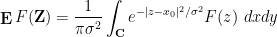
. Similarly, a complex random variable {\mathbf{Z}} is said to be normally distributed with mean {z_0 \in {\bf R}} and variance {\sigma^2>0} if one has

\displaystyle  \mathop{\bf E} F(\mathbf{Z}) = \frac{1}{\pi \sigma^2} \int_{\bf C} e^{-|z-x_0|^2/\sigma^2} F(z)\ dx dy

for all test functions {F \in C_c({\bf C})}, where {dx dy} is the area element on {{\bf C}}.
A real Brownian motion with base point {x_0 \in {\bf R}} is a random, almost surely continuous function {\mathbf{B}^{x_0}: [0,+\infty) \rightarrow {\bf R}} (using the locally uniform topology on continuous functions) with the property that (almost surely) {\mathbf{B}^{x_0}(0) = x_0}, and for any sequence of times {0 \leq t_0 < t_1 < t_2 < \dots < t_n}, the increments {\mathbf{B}^{x_0}(t_i) - \mathbf{B}^{x_0}(t_{i-1})} for {i=1,\dots,n} are independent real random variables that are normally distributed with mean zero and variance {t_i - t_{i-1}}. Similarly, a complex Brownian motion with base point {z_0 \in {\bf R}} is a random, almost surely continuous function {\mathbf{B}^{z_0}: [0,+\infty) \rightarrow {\bf R}} with the property that {\mathbf{B}^{z_0}(0) = z_0} and for any sequence of times {0 \leq t_0 < t_1 < t_2 < \dots < t_n}, the increments {\mathbf{B}^{z_0}(t_i) - \mathbf{B}^{z_0}(t_{i-1})} for {i=1,\dots,n} are independent complex random variables that are normally distributed with mean zero and variance {t_i - t_{i-1}}.

Remark 2 Thanks to the central limit theorem, the hypothesis that the increments {\mathbf{B}^{x_0}(t_i) - \mathbf{B}^{x_0}(t_{i-1})} be normally distributed can be dropped from the definition of a Brownian motion, so long as one retains the independence and the normalisation of the mean and variance (technically one also needs some uniform integrability on the increments beyond the second moment, but we will not detail this here). A similar statement is also true for the complex Brownian motion (where now we need to normalise the variances and covariances of the real and imaginary parts of the increments).

Real and complex Brownian motions exist from any base point {x_0} or {z_0}; see e.g. this previous blog post for a construction. We have the following simple invariances:

Exercise 3

  • (i) (Translation invariance) If {\mathbf{B}^{x_0}} is a real Brownian motion with base point {x_0 \in {\bf R}}, and {h \in {\bf R}}, show that {\mathbf{B}^{x_0}+h} is a real Brownian motion with base point {x_0+h}. Similarly, if {\mathbf{B}^{z_0}} is a complex Brownian motion with base point {z_0 \in {\bf R}}, and {h \in {\bf C}}, show that {\mathbf{B}^{z_0}+c} is a complex Brownian motion with base point {z_0+h}.
  • (ii) (Dilation invariance) If {\mathbf{B}^{0}} is a real Brownian motion with base point {0}, and {\lambda \in {\bf R}} is non-zero, show that {t \mapsto \lambda \mathbf{B}^0(t / |\lambda|^{1/2})} is also a real Brownian motion with base point {0}. Similarly, if {\mathbf{B}^0} is a complex Brownian motion with base point {0}, and {\lambda \in {\bf C}} is non-zero, show that {t \mapsto \lambda \mathbf{B}^0(t / |\lambda|^{1/2})} is also a complex Brownian motion with base point {0}.
  • (iii) (Real and imaginary parts) If {\mathbf{B}^0} is a complex Brownian motion with base point {0}, show that {\sqrt{2} \mathrm{Re} \mathbf{B}^0} and {\sqrt{2} \mathrm{Im} \mathbf{B}^0} are independent real Brownian motions with base point {0}. Conversely, if {\mathbf{B}^0_1, \mathbf{B}^0_2} are independent real Brownian motions of base point {0}, show that {\frac{1}{\sqrt{2}} (\mathbf{B}^0_1 + i \mathbf{B}^0_2)} is a complex Brownian motion with base point {0}.

The next lemma is a special case of the optional stopping theorem.

Lemma 4 (Optional stopping identities)

  • (i) (Real case) Let {\mathbf{B}^{x_0}} be a real Brownian motion with base point {x_0 \in {\bf R}}. Let {\mathbf{t}} be a bounded stopping time – a bounded random variable with the property that for any time {t \geq 0}, the event that {\mathbf{t} \leq t} is determined by the values of the trajectory {\mathbf{B}^{x_0}} for times up to {t} (or more precisely, this event is measurable with respect to the {\sigma} algebra generated by this proprtion of the trajectory). Then

    \displaystyle  \mathop{\bf E} \mathbf{B}^{x_0}(\mathbf{t}) = x_0

    and

    \displaystyle  \mathop{\bf E} (\mathbf{B}^{x_0}(\mathbf{t})-x_0)^2 - \mathbf{t} = 0

    and

    \displaystyle  \mathop{\bf E} (\mathbf{B}^{x_0}(\mathbf{t})-x_0)^4 = O( \mathop{\bf E} \mathbf{t}^2 ).

  • (ii) (Complex case) Let {\mathbf{B}^{z_0}} be a real Brownian motion with base point {z_0 \in {\bf R}}. Let {\mathbf{t}} be a bounded stopping time – a bounded random variable with the property that for any time {t \geq 0}, the event that {\mathbf{t} \leq t} is determined by the values of the trajectory {\mathbf{B}^{x_0}} for times up to {t}. Then

    \displaystyle  \mathop{\bf E} \mathbf{B}^{z_0}(\mathbf{t}) = z_0

    \displaystyle  \mathop{\bf E} (\mathrm{Re}(\mathbf{B}^{z_0}(\mathbf{t})-z_0))^2 - \frac{1}{2} \mathbf{t} = 0

    \displaystyle  \mathop{\bf E} (\mathrm{Im}(\mathbf{B}^{z_0}(\mathbf{t})-z_0))^2 - \frac{1}{2} \mathbf{t} = 0

    \displaystyle  \mathop{\bf E} \mathrm{Re}(\mathbf{B}^{z_0}(\mathbf{t})-z_0) \mathrm{Im}(\mathbf{B}^{z_0}(\mathbf{t})-z_0) = 0

    \displaystyle  \mathop{\bf E} |\mathbf{B}^{x_0}(\mathbf{t})-z_0|^4 = O( \mathop{\bf E} \mathbf{t}^2 ).

Proof: (Slightly informal) We just prove (i) and leave (ii) as an exercise. By translation invariance we can take {x_0=0}. Let {T} be an upper bound for {\mathbf{t}}. Since {\mathbf{B}^0(T)} is a real normally distributed variable with mean zero and variance {T}, we have

\displaystyle  \mathop{\bf E} \mathbf{B}^0( T ) = 0

and

\displaystyle  \mathop{\bf E} \mathbf{B}^0( T )^2 = T

and

\displaystyle  \mathop{\bf E} \mathbf{B}^0( T )^4 = 3T^2.

By the law of total expectation, we thus have

\displaystyle  \mathop{\bf E} \mathop{\bf E}(\mathbf{B}^0( T ) | \mathbf{t}, \mathbf{B}^{z_0}(\mathbf{t}) ) = 0

and

\displaystyle  \mathop{\bf E} \mathop{\bf E}((\mathbf{B}^0( T ))^2 | \mathbf{t}, \mathbf{B}^{z_0}(\mathbf{t}) ) = T

and

\displaystyle  \mathop{\bf E} \mathop{\bf E}((\mathbf{B}^0( T ))^4 | \mathbf{t}, \mathbf{B}^{z_0}(\mathbf{t}) ) = 3T^2

where the inner conditional expectations are with respect to the event that {\mathbf{t}, \mathbf{B}^{0}(\mathbf{t})} attains a particular point in {S}. However, from the independent increment nature of Brownian motion, once one conditions {(\mathbf{t}, \mathbf{B}^{0}(\mathbf{t}))} to a fixed point {(t, x)}, the random variable {\mathbf{B}^0(T)} becomes a real normally distributed variable with mean {x} and variance {T-t}. Thus we have

\displaystyle  \mathop{\bf E}(\mathbf{B}^0( T ) | \mathbf{t}, \mathbf{B}^{z_0}(\mathbf{t}) ) = \mathbf{B}^{z_0}(\mathbf{t})

and

\displaystyle  \mathop{\bf E}( (\mathbf{B}^0( T ))^2 | \mathbf{t}, \mathbf{B}^{z_0}(\mathbf{t}) ) = \mathbf{B}^{z_0}(\mathbf{t})^2 + T - \mathbf{t}

and

\displaystyle  \mathop{\bf E}( (\mathbf{B}^0( T ))^4 | \mathbf{t}, \mathbf{B}^{z_0}(\mathbf{t}) ) = \mathbf{B}^{z_0}(\mathbf{t})^4 + 6(T - \mathbf{t}) \mathbf{B}^{z_0}(\mathbf{t})^2 + 3(T - \mathbf{t})^2

which give the first two claims, and (after some algebra) the identity

\displaystyle  \mathop{\bf E} \mathbf{B}^{z_0}(\mathbf{t})^4 - 6 \mathbf{t} \mathbf{B}^{z_0}(\mathbf{t})^2 + 3 \mathbf{t}^2 = 0

which then also gives the third claim. \Box

Exercise 5 Prove the second part of Lemma 4.

Read the rest of this entry »

Previous set of notes: Notes 4. Next set of notes: 246B Notes 1.
In the previous set of notes we introduced the notion of a complex diffeomorphism {f: U \rightarrow V} between two open subsets {U,V} of the complex plane {{\bf C}} (or more generally, two Riemann surfaces): an invertible holomorphic map whose inverse was also holomorphic. (Actually, the last part is automatic, thanks to Exercise 41 of Notes 4.) Such maps are also known as biholomorphic maps or conformal maps (although in some literature the notion of “conformal map” is expanded to permit maps such as the complex conjugation map {z \mapsto \overline{z}} that are angle-preserving but not orientation-preserving, as well as maps such as the exponential map {z \mapsto \exp(z)} from {{\bf C}} to {{\bf C} \backslash \{0\}} that are only locally injective rather than globally injective). Such complex diffeomorphisms can be used in complex analysis (or in the analysis of harmonic functions) to change the underlying domain {U} to a domain that may be more convenient for calculations, thanks to the following basic lemma:

Lemma 1 (Holomorphicity and harmonicity are conformal invariants) Let {\phi: U \rightarrow V} be a complex diffeomorphism between two Riemann surfaces {U,V}.

  • (i) If {f: V \rightarrow W} is a function to another Riemann surface {W}, then {f} is holomorphic if and only if {f \circ \phi: U \rightarrow W} is holomorphic.
  • (ii) If {U,V} are open subsets of {{\bf C}} and {u: V \rightarrow {\bf R}} is a function, then {u} is harmonic if and only if {u \circ \phi: U \rightarrow {\bf R}} is harmonic.

Proof: Part (i) is immediate since the composition of two holomorphic functions is holomorphic. For part (ii), observe that if {u: V \rightarrow {\bf R}} is harmonic then on any ball {B(z_0,r)} in {V}, {u} is the real part of some holomorphic function {f: B(z_0,r) \rightarrow {\bf C}} thanks to Exercise 62 of Notes 3. By part (i), {f \circ \phi: \phi^{-1}(B(z_0,r)) \rightarrow {\bf C}} is also holomorphic. Taking real parts we see that {u \circ \phi} is harmonic on each ball preimage {\phi^{-1}(B(z_0,r))} in {V}, and hence harmonic on all of {V}, giving one direction of (ii); the other direction is proven similarly. \Box

Exercise 2 Establish Lemma 1(ii) by direct calculation, avoiding the use of holomorphic functions. (Hint: the calculations are cleanest if one uses Wirtinger derivatives, as per Exercise 27 of Notes 1.)

Exercise 3 Let {\phi: U \rightarrow V} be a complex diffeomorphism between two open subsets {U,V} of {{\bf C}}, let {z_0} be a point in {U}, let {m} be a natural number, and let {f: V \rightarrow {\bf C} \cup \{\infty\}} be holomorphic. Show that {f: V \rightarrow {\bf C} \cup \{\infty\}} has a zero (resp. a pole) of order {m} at {\phi(z_0)} if and only if {f \circ \phi: U \rightarrow {\bf C} \cup \{\infty\}} has a zero (resp. a pole) of order {m} at {z_0}.

From Lemma 1(ii) we can now define the notion of a harmonic function {u: M \rightarrow {\bf R}} on a Riemann surface {M}; such a function {u} is harmonic if, for every coordinate chart {\phi_\alpha: U_\alpha \rightarrow V_\alpha} in some atlas, the map {u \circ \phi_\alpha^{-1}: V_\alpha \rightarrow {\bf R}} is harmonic. Lemma 1(ii) ensures that this definition of harmonicity does not depend on the choice of atlas. Similarly, using Exercise 3 one can define what it means for a holomorphic map {f: M \rightarrow {\bf C} \cup \{\infty\}} on a Riemann surface {M} to have a pole or zero of a given order at a point {p_0 \in M}, with the definition being independent of the choice of atlas; we can also identify such functions as equivalence classes of meromorphic functions {f: M \backslash S \rightarrow {\bf C}} in complete analogy with the case of meromorphic functions on domains {U}. Finally, we can define the notion of an essential singularity of a holomorphic function {f: M \backslash S \rightarrow {\bf C}} at some isolated singularity {p \in S} in a Riemann surface as one that cannot be extended to a holomorphic function {f: (M \backslash S) \cup \{p\} \rightarrow{\bf C} \cup \{\infty\}}.
In view of Lemma 1, it is thus natural to ask which Riemann surfaces are complex diffeomorphic to each other, and more generally to understand the space of holomorphic maps from one given Riemann surface to another. We will initially focus attention on three important model Riemann surfaces:

  • (i) (Elliptic model) The Riemann sphere {{\bf C} \cup \{\infty\}};
  • (ii) (Parabolic model) The complex plane {{\bf C}}; and
  • (iii) (Hyperbolic model) The unit disk {D(0,1)}.

The designation of these model Riemann surfaces as elliptic, parabolic, and hyperbolic comes from Riemannian geometry, where it is natural to endow each of these surfaces with a constant curvature Riemannian metric which is positive, zero, or negative in the elliptic, parabolic, and hyperbolic cases respectively. However, we will not discuss Riemannian geometry further here.
All three model Riemann surfaces are simply connected, but none of them are complex diffeomorphic to any other; indeed, there are no non-constant holomorphic maps from the Riemann sphere to the plane or the disk, nor are there any non-constant holomorphic maps from the plane to the disk (although there are plenty of holomorphic maps going in the opposite directions). The complex automorphisms (that is, the complex diffeomorphisms from a surface to itself) of each of the three surfaces can be classified explicitly. The automorphisms of the Riemann sphere turn out to be the Möbius transformations {z \mapsto \frac{az+b}{cz+d}} with {ad-bc \neq 0}, also known as fractional linear transformations. The automorphisms of the complex plane are the linear transformations {z \mapsto az+b} with {a \neq 0}, and the automorphisms of the disk are the fractional linear transformations of the form {z \mapsto e^{i\theta} \frac{\alpha - z}{1 - \overline{\alpha} z}} for {\theta \in {\bf R}} and {\alpha \in D(0,1)}. Holomorphic maps {f: D(0,1) \rightarrow D(0,1)} from the disk {D(0,1)} to itself that fix the origin obey a basic but incredibly important estimate known as the Schwarz lemma: they are “dominated” by the identity function {z \mapsto z} in the sense that {|f(z)| \leq |z|} for all {z \in D(0,1)}. Among other things, this lemma gives guidance to determine when a given Riemann surface is complex diffeomorphic to a disk; we shall discuss this point further below.
It is a beautiful and fundamental fact in complex analysis that these three model Riemann surfaces are in fact an exhaustive list of the simply connected Riemann surfaces, up to complex diffeomorphism. More precisely, we have the Riemann mapping theorem and the uniformisation theorem:

Theorem 4 (Riemann mapping theorem) Let {U} be a simply connected open subset of {{\bf C}} that is not all of {{\bf C}}. Then {U} is complex diffeomorphic to {D(0,1)}.

Theorem 5 (Uniformisation theorem) Let {M} be a simply connected Riemann surface. Then {M} is complex diffeomorphic to {{\bf C} \cup \{\infty\}}, {{\bf C}}, or {D(0,1)}.

As we shall see, every connected Riemann surface can be viewed as the quotient of its simply connected universal cover by a discrete group of automorphisms known as deck transformations. This in principle gives a complete classification of Riemann surfaces up to complex diffeomorphism, although the situation is still somewhat complicated in the hyperbolic case because of the wide variety of discrete groups of automorphisms available in that case.
We will prove the Riemann mapping theorem in these notes, using the elegant argument of Koebe that is based on the Schwarz lemma and Montel’s theorem (Exercise 58 of Notes 4). The uniformisation theorem is however more difficult to establish; we discuss some components of a proof (based on the Perron method of subharmonic functions) here, but stop short of providing a complete proof.
The above theorems show that it is in principle possible to conformally map various domains into model domains such as the unit disk, but the proofs of these theorems do not readily produce explicit conformal maps for this purpose. For some domains we can just write down a suitable such map. For instance:

Exercise 6 (Cayley transform) Let {{\bf H} := \{ z \in {\bf C}: \mathrm{Im} z > 0 \}} be the upper half-plane. Show that the Cayley transform {\phi: {\bf H} \rightarrow D(0,1)}, defined by

\displaystyle  \phi(z) := \frac{z-i}{z+i},

is a complex diffeomorphism from the upper half-plane {{\bf H}} to the disk {D(0,1)}, with inverse map {\phi^{-1}: D(0,1) \rightarrow {\bf H}} given by

\displaystyle  \phi^{-1}(w) := i \frac{1+w}{1-w}.

Exercise 7 Show that for any real numbers {a<b}, the strip {\{ z \in {\bf C}: a < \mathrm{Re}(z) < b \}} is complex diffeomorphic to the disk {D(0,1)}. (Hint: use the complex exponential and a linear transformation to map the strip onto the half-plane {{\bf H}}.)

Exercise 8 Show that for any real numbers {a<b<a+2\pi}, the strip {\{ re^{i\theta}: r>0, a < \theta < b \}} is complex diffeomorphic to the disk {D(0,1)}. (Hint: use a branch of either the complex logarithm, or of a complex power {z \mapsto z^\alpha}.)

We will discuss some other explicit conformal maps in this set of notes, such as the Schwarz-Christoffel maps that transform the upper half-plane {{\bf H}} to polygonal regions. Further examples of conformal mapping can be found in the text of Stein-Shakarchi.
Read the rest of this entry »

Archives