Given a random variable  that takes on only finitely many values, we can define its Shannon entropy by the formula
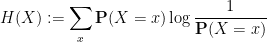
with the convention that  . (In some texts, one uses the logarithm to base
  rather than the natural logarithm, but the choice of base will not be relevant for this discussion.) This is clearly a nonnegative quantity. Given two random variables
  taking on finitely many values, the joint variable
  is also a random variable taking on finitely many values, and also has an entropy
  . It obeys the Shannon inequalities

so we can define some further nonnegative quantities, the mutual information

and the conditional entropies

More generally, given three random variables  , one can define the conditional mutual information

and the final of the Shannon entropy inequalities asserts that this quantity is also non-negative.
The mutual information  is a measure of the extent to which and
  fail to be independent; indeed, it is not difficult to show that vanishes if and only if and are independent. Similarly,
  vanishes if and only if and are conditionally independent relative to
  . At the other extreme,
  is a measure of the extent to which fails to depend on ; indeed, it is not difficult to show that
  if and only if is determined by in the sense that there is a deterministic function
  such that
  . In a related vein, if and
  are equivalent in the sense that there are deterministic functional relationships
  ,
,  between the two variables, then is interchangeable with for the purposes of computing the above quantities, thus for instance
  ,
,  ,
,  ,
,  , etc..
One can get some initial intuition for these information-theoretic quantities by specialising to a simple situation in which all the random variables being considered come from restricting a single random (and uniformly distributed) boolean function  on a given finite domain
  to some subset
  of :
of :

In this case, has the law of a random uniformly distributed boolean function from to  , and the entropy here can be easily computed to be
  , where
  denotes the cardinality of . If is the restriction of
  to , and is the restriction of to
  , then the joint variable is equivalent to the restriction of to
  . If one discards the normalisation factor
  , one then obtains the following dictionary between entropy and the combinatorics of finite sets:
| Random variables |
Finite sets  |
Entropy  |
Cardinality |
| Joint variable |
Union |
| Mutual information |
Intersection cardinality  |
| Conditional entropy |
Set difference cardinality  |
| Conditional mutual information |
 |
 independent independent |
 disjoint disjoint |
| determined by |
a subset of |
| conditionally independent relative to |
 |
Every (linear) inequality or identity about entropy (and related quantities, such as mutual information) then specialises to a combinatorial inequality or identity about finite sets that is easily verified. For instance, the Shannon inequality  becomes the union bound
 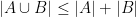 , and the definition of mutual information becomes the inclusion-exclusion formula

For a more advanced example, consider the data processing inequality that asserts that if  are conditionally independent relative to , then
  . Specialising to sets, this now says that if
  are disjoint outside of , then
  ; this can be made apparent by considering the corresponding Venn diagram. This dictionary also suggests how to prove the data processing inequality using the existing Shannon inequalities. Firstly, if and
  are not necessarily disjoint outside of , then a consideration of Venn diagrams gives the more general inequality

and a further inspection of the diagram then reveals the more precise identity

Using the dictionary in the reverse direction, one is then led to conjecture the identity

which (together with non-negativity of conditional mutual information) implies the data processing inequality, and this identity is in turn easily established from the definition of mutual information.
On the other hand, not every assertion about cardinalities of sets generalises to entropies of random variables that are not arising from restricting random boolean functions to sets. For instance, a basic property of sets is that disjointness from a given set is preserved by unions:

Indeed, one has the union bound

Applying the dictionary in the reverse direction, one might now conjecture that if was independent of and was independent of , then should also be independent of , and furthermore that

but these statements are well known to be false (for reasons related to pairwise independence of random variables being strictly weaker than joint independence). For a concrete counterexample, one can take  to be independent, uniformly distributed random elements of the finite field
  of two elements, and take
  to be the sum of these two field elements. One can easily check that each of and is separately independent of , but the joint variable determines and thus is not independent of .
From the inclusion-exclusion identities


one can check that (1) is equivalent to the trivial lower bound  . The basic issue here is that in the dictionary between entropy and combinatorics, there is no satisfactory entropy analogue of the notion of a triple intersection
  . (Even the double intersection
  only exists information theoretically in a “virtual” sense; the mutual information allows one to “compute the entropy” of this “intersection”, but does not actually describe this intersection itself as a random variable.)
However, this issue only arises with three or more variables; it is not too difficult to show that the only linear equalities and inequalities that are necessarily obeyed by the information-theoretic quantities  associated to just two variables are those that are also necessarily obeyed by their combinatorial analogues
  . (See for instance the Venn diagram at the Wikipedia page for mutual information for a pictorial summation of this statement.)
One can work with a larger class of special cases of Shannon entropy by working with random linear functions rather than random boolean functions. Namely, let  be some finite-dimensional vector space over a finite field
  , and let
  be a random linear functional on , selected uniformly among all such functions. Every subspace
  of then gives rise to a random variable
  formed by restricting to . This random variable is also distributed uniformly amongst all linear functions on , and its entropy can be easily computed to be
  . Given two random variables formed by restricting to
  respectively, the joint random variable determines the random linear function on the union
  on the two spaces, and thus by linearity on the Minkowski sum
  as well; thus is equivalent to the restriction of to . In particular,
  . This implies that
  and also
  , where
  is the quotient map. After discarding the normalising constant
  , this leads to the following dictionary between information theoretic quantities and linear algebra quantities, analogous to the previous dictionary:
| Random variables |
Subspaces  |
| Entropy |
Dimension  |
| Joint variable |
Sum |
| Mutual information |
Dimension of intersection  |
| Conditional entropy |
Dimension of projection  |
| Conditional mutual information |
 |
| independent |
transverse ( ) ) |
| determined by |
a subspace of  |
| conditionally independent relative to |
 , ,  transverse. transverse. |
The combinatorial dictionary can be regarded as a specialisation of the linear algebra dictionary, by taking to be the vector space  over the finite field
  of two elements, and only considering those subspaces that are coordinate subspaces
  associated to various subsets of .
As before, every linear inequality or equality that is valid for the information-theoretic quantities discussed above, is automatically valid for the linear algebra counterparts for subspaces of a vector space over a finite field by applying the above specialisation (and dividing out by the normalising factor of ). In fact, the requirement that the field be finite can be removed by applying the compactness theorem from logic (or one of its relatives, such as Los’s theorem on ultraproducts, as done in this previous blog post).
The linear algebra model captures more of the features of Shannon entropy than the combinatorial model. For instance, in contrast to the combinatorial case, it is possible in the linear algebra setting to have subspaces such that and are separately transverse to  , but their sum is not; for instance, in a two-dimensional vector space
  , one can take to be the one-dimensional subspaces spanned by
  ,
,  , and
, and  respectively. Note that this is essentially the same counterexample from before (which took
  to be the field of two elements). Indeed, one can show that any necessarily true linear inequality or equality involving the dimensions of three subspaces (as well as the various other quantities on the above table) will also be necessarily true when applied to the entropies of three discrete random variables (as well as the corresponding quantities on the above table).
However, the linear algebra model does not completely capture the subtleties of Shannon entropy once one works with four or more variables (or subspaces). This was first observed by Ingleton, who established the dimensional inequality

for any subspaces  . This is easiest to see when the three terms on the right-hand side vanish; then
  are transverse, which implies that
  ; similarly
  . But and are transverse, and this clearly implies that and are themselves transverse. To prove the general case of Ingleton’s inequality, one can define
  and use
  (and similarly for instead of ) to reduce to establishing the inequality

which can be rearranged using  (and similarly for instead of ) and
  as
as

but this is clear since  .
.
Returning to the entropy setting, the analogue

of (3) is true (exercise!), but the analogue

of Ingleton’s inequality is false in general. Again, this is easiest to see when all the terms on the right-hand side vanish; then are conditionally independent relative to , and relative to , and and are independent, and the claim (4) would then be asserting that and are independent. While there is no linear counterexample to this statement, there are simple non-linear ones: for instance, one can take  to be independent uniform variables from , and take and to be (say)
  and
and  respectively (thus are the indicators of the events
  and
and  respectively). Once one conditions on either or , one of has positive conditional entropy and the other has zero entropy, and so are conditionally independent relative to either or ; also, or are independent of each other. But and are not independent of each other (they cannot be simultaneously equal to
  ). Somehow, the feature of the linear algebra model that is not present in general is that in the linear algebra setting, every pair of subspaces has a well-defined intersection
  that is also a subspace, whereas for arbitrary random variables , there does not necessarily exist the analogue of an intersection, namely a “common information” random variable that has the entropy of and is determined either by or by .
I do not know if there is any simpler model of Shannon entropy that captures all the inequalities available for four variables. One significant complication is that there exist some information inequalities in this setting that are not of Shannon type, such as the Zhang-Yeung inequality


One can however still use these simpler models of Shannon entropy to be able to guess arguments that would work for general random variables. An example of this comes from my paper on the logarithmically averaged Chowla conjecture, in which I showed among other things that
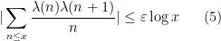
whenever  was sufficiently large depending on
  , where
  is the Liouville function. The information-theoretic part of the proof was as follows. Given some intermediate scale
  between and , one can form certain random variables
  . The random variable
  is a sign pattern of the form
  where
where  is a random number chosen from to (with logarithmic weighting). The random variable
  was tuple
  of reductions of to primes
  comparable to
  . Roughly speaking, what was implicitly shown in the paper (after using the multiplicativity of , the circle method, and the Matomaki-Radziwill theorem on short averages of multiplicative functions) is that if the inequality (5) fails, then there was a lower bound

on the mutual information between and . From translation invariance, this also gives the more general lower bound
for any  , where
  denotes the shifted sign pattern
  . On the other hand, one had the entropy bounds

and from concatenating sign patterns one could see that  is equivalent to the joint random variable
  for any
  . Applying these facts and using an “entropy decrement” argument, I was able to obtain a contradiction once was allowed to become sufficiently large compared to
  , but the bound was quite weak (coming ultimately from the unboundedness of
  as the interval
 ![{[H_-,H_+]}](https://s0.wp.com/latex.php?latex=%7B%5BH_-%2CH_%2B%5D%7D&bg=ffffff&fg=000000&s=0&c=20201002) of values of under consideration becomes large), something of the order of
of values of under consideration becomes large), something of the order of  ; the quantity needs at various junctures to be less than a small power of
  , so the relationship between and becomes essentially quadruple exponential in nature,
  . The basic strategy was to observe that the lower bound (6) causes some slowdown in the growth rate
  of the mean entropy, in that this quantity decreased by
  as
as  increased from to
  , basically by dividing
  into components
  ,
,  and observing from (6) each of these shares a bit of common information with the same variable . This is relatively clear when one works in a set model, in which is modeled by a set
  of size
  , and is modeled by a set of the form

for various sets  of size
  (also there is some translation symmetry that maps to a shift
  while preserving all of the ).
However, on considering the set model recently, I realised that one can be a little more efficient by exploiting the fact (basically the Chinese remainder theorem) that the random variables are basically jointly independent as ranges over dyadic values that are much smaller than , which in the set model corresponds to the all being disjoint. One can then establish a variant

of (6), which in the set model roughly speaking asserts that each claims a portion of the  of cardinality
  that is not claimed by previous choices of . This leads to a more efficient contradiction (relying on the unboundedness of
  rather than ) that looks like it removes one order of exponential growth, thus the relationship between and is now
  . Returning to the entropy model, one can use (7) and Shannon inequalities to establish an inequality of the form

for a small constant  , which on iterating and using the boundedness of
  gives the claim. (A modification of this analysis, at least on the level of the back of the envelope calculation, suggests that the Matomaki-Radziwill theorem is needed only for ranges greater than
  or so, although at this range the theorem is not significantly simpler than the general case).


29 comments
Comments feed for this article
1 March, 2017 at 12:25 pm
Manny
I think the equation in first sentence is missing a minus.
1 March, 2017 at 12:28 pm
Nikita Sidorov
In the first formula the minus is missing.
1 March, 2017 at 12:29 pm
Nikita Sidorov
Sorry, didn’t notice 1/… It’s all good, then.
1 March, 2017 at 1:06 pm
Ravi Andrew Bajaj
Dear Professor Tao,
Are there applications of this result to random matrix theory?
–RAB
1 March, 2017 at 1:46 pm
Nick Cook
Nice post! Just to note a couple of typos: In the third line of the dictionary for subspaces, either change the random variable to its entropy or the dimension to a subspace. In the paragraph below (5) I think you mean “if the inequality (5) fails…”
[Corrected, thanks – T.]
1 March, 2017 at 3:01 pm
.
Your dictionary as in other dictionaries misses the non-trivial $X,Y,Z$ are correlated case. How would you give a dictionary between information theory and set theory/subspace for the cases $X,Y,Z$ are correlated?
1 March, 2017 at 10:16 pm
domotorp
What happens if we swap union and intersection in the set dictionary, or we project ONTO the subspaces in the subspace dictionary? Is it only that some inequalities and signs turn?
Also, I think there are a few more typos:
1, if and if -> if and only if
2, equivalent to the restriction to f -> of f
3, S/U is the quotient map -> S/V
2 March, 2017 at 9:43 am
Terence Tao
Thanks for the corrections!
In the set dictionary, one can replace all the sets with their complements
  in the ambient space
  . This interchanges unions and intersections by de Morgan’s laws, but also cardinality
  must now be replaced by cocardinality
  . The analogue of conditional entropy
  is now the cocardinality of
  inside
  (viewing the latter as the new ambient space, thus conditioning corresponds to restricting the ambient space and all the sets inside it to
  ).
).
Similarly, in the linear algebra dictionary, by replacing all the vector spaces with their complements (viewed as subspaces of the dual space , or if one has a nondegenerate bilinear form on
  one can take orthogonal complements with respect to that form and stay inside
  ), one can interchange sums and intersections, replacing dimensions with codimensions throughout. Again, the analogue of projection is now restriction (restricting the ambient space
  and all of its subspaces to a smaller space
  ). For instance, the analogue of conditional entropy
  is now the codimension of
  inside
  .
.
1 March, 2017 at 10:25 pm
Djdkd
Dear Terry, I think you proved something considerably stronger than (5)
2 March, 2017 at 3:53 am
Anonymous
In the second paragraph, the word only is missing in “…vanishes if and if …”
2 March, 2017 at 6:47 am
John Fries
Professor Tao,
Have you read Amari’s paper “Information Geometry on Hierarchy of Probability Distributions”? Instead of mapping information theory to set theory or linear algebra, he maps it to differential geometry. Of particular note is that he is able to discuss triplewise and higher interactions between random variables.
Here is a link: https://pdfs.semanticscholar.org/aa12/aee8cb3fb5ef2c545c0a9efa383326270340.pdf
Sincerely,
John Fries
3 March, 2017 at 5:29 pm
Jeff
most readers of this blog probably won’t get confused by this, but it’s slightly confusing to call conditional entropy “relative entropy”, which many take as synonymous with the fairly unrelated concept of KL divergence.
[Corrected, thanks – T.]
4 March, 2017 at 6:13 am
Oliver Knill
Nice analogies. Since cardinality is generalized by Euler characteristic for finite abstract simplicial complexes, one could push the analogy even further. The inclusion-exclusion formula becomes the property of a “valuation” on complexes which is the defining relation. Valuation is understood in the sense of Klain and Rota, who developed the discrete analogue of continuum geometric probability theory. Zero dimensional complexes are sets so that this extends the finite set analogy.
Entropy, an important functional (maybe the most important one) in a probabilistic set-up when dealing with random variables X is then linked to Euler characteristic an important quantity (maybe the most important one) in topology, when dealing with simplicial complexes X.
Euler characteristic has long known to be the only valuation which is invariant under Barycentric refinement of the complex G, the complex, in which the sets of G are the points of the new base and the new sets are the subsets. The reason is that there is a universal linear map A which maps the f-vector of G to the f-vector of the refinement of G. This matrix A has a unique eigenvalue 1 which is (1,-1,1,-1,…) leading to the Euler characteristic. Euler characteristic is then a Perron-Frobenius eigenvector of the inverse of the Barycentric refinement operator. It is unique if one normalizes it so that its value on a 1-point complex 1 is 1.
There is a similar defining renormalization picture for entropy: Shannon in his 1948 article already established such a condition which defines entropy uniquely (Theorem 2 in his paper). Much earlier, Boltzmann saw entropy as a functional on measures as he defined it as the expectation of -log(P) (famously displayed on his tomb stone) and already on physical grounds wanted entropy to be additive for physical systems which do not interact Taking about random variables X means the entropy of its law (which essentially corresponds to the Shannon condition). Obviously, entropy H satisfies H(X+X’)/2=H(X) if X,X’ are IID and H(X)=0 if X is a constant random variable. This renormalisation operator X -> X+X’ is the analogue of Barycentric refinement and the requirement H(X+X’)/2=H(X) defines the entropy functional uniquely if normalized for the constant random variable. (Shannon seems to have a stronger assumptions I(X:Y)=0 for independent X,Y but this could be bootstrapped from H(X+X’)/2=H(X) for IID X,X’ using polarization from H(X+Y + X’+Y’)). The value H=-log(X) for Euler characteristic X is an analogue of entropy as it is additive with respect to Cartesian products of complexes but topologists refrain from taking the log as we also want to deal with spaces of Euler characteristic 0 like the circle. A special case is the product G x 1 with one-point complex 1 which is the Barycentric refinement of G. The analogue of H(A + B)=H(A) + H(B) for IID random variables A,B is H(A x B) = H(A) + H(B) for simplicial complexes. The analogue of H(1)=0 (H=entropy, 1=constant random variable) is H(1)=0 (H=-log(Euler characteristic, 1=1 point complex)).
There is also an analogue central limit theorem: the operator X -> X+X’ for random variables (X’ is just an IID copy of X and X+X’ is normalized to have variance 1 obviously leads to the classical central limit theorem and entropy is a Lyapunov function under the operation and iterating the map is a discrete time gradient type flow leading to a Gaussian distribution, the maximum. Similarly as a random variable X defines a law P, any simplicial complex X has a “law” P: it is the density of states of its Laplacian, a discrete point measure P on the real line. What happens during Barycentric refinement is that one is close to adding up independent complexes (there is a boundary part which becomes negligible and controlling this needs a Lidskii-Last inequality). The story is even more intriguing as in probability theory because so far, we only know the limiting measure for one-dimensional complexes. It is the potential theoretical equilibrium measure on an interval, the arcsine law. The limiting universal measures for higher dimensional complexes depends only on the maximal dimension of the complex and are unidentified so far. Its integrated density of states (= CDF) appears discontinuous in dimensions larger than 1.
4 March, 2017 at 5:22 pm
Shannon Entropy and Euler Characteristic - Quantum Calculus
[…] A blog entry mentions some analogies between entropy and other combinatorial notions. One can push the analogy in an other direction and compare random variables with simplicial complexes, Shannon entropy with Euler characteristic. […]
5 March, 2017 at 10:39 am
Furstenberg limits of the Liouville function | What's new
[…] of ) shows that eventually becomes negative for sufficiently large , which is absurd. (See also this previous blog post for a sketch of a slightly different way to conclude the argument from entropy […]
8 March, 2017 at 12:24 pm
Machine Learning Notes/Pointers | SChaiken's Blog
[…] Terry Tao on Shannon Entropy and its analogies to set functions […]
19 March, 2017 at 12:14 pm
Joe Triscari
Interesting article.
It makes me wonder if there are category theoretic ideas to be milked out of these analogies.
The free vector space on a set preserves entropy. Maybe there’s some entropy concept lurking under other categories and there are functors that preserve the entropy…
22 March, 2017 at 1:25 am
David Tse
Nice post. A pedagogical comment. Instead of defining the set theoretic model in terms of a random mapping F, wouldn’t it be more straightforward to define it in terms of a set of i.i.d. Bern(0.5) random variables , where $n = |\Omega|$? Then for every subset
  , one can define a random vector
  .
.
[One could indeed do this, but I preferred to use the random function model as it made the similarity between the set theoretic dictionary and the linear algebra dictionary more apparent. -T.]
24 March, 2017 at 4:58 am
David Tse
Continuing on my previous comment and in response to Terry’s note, I believe the representation of the set theoretic model in terms of basic random variables can be generalized to the linear algebra model by starting again with
  but now thinking it as a random vector X. For each linear transformation T, we can define
  . The set theoretic model corresponds to the random vectors obtained by restricting T to be diagonal with only 1’s and 0’s.
23 March, 2017 at 6:54 pm
Raymond Yeung
Nice post by Terry and others. Here are some supplementary comments.
1. The first rigorous proof of the set-entropy dictionary, to my knowledge, is the 1962 paper by Hu (originally in Russian):
http://epubs.siam.org/doi/pdf/10.1137/1107041
2. The analogy between sets and entropy was enhanced into an equivalence in my 1991 paper. For a fixed finite set of discrete random variables, we have for example
$I(X:Y|Z) = \mu^*(A \cap B – C)$ ,
where $\mu^*$, called the I-Measure, is a unique signed measure defined on a suitably constructed $\sigma$-field. $\mu^*$ is unique in the sense that
it is determined by the joint entropies of all the random variables involved. With this equivalence, one can formally apply all the tools in set theory to information theory. In short, in the information theory domain, every identity (not inequality) that one can read off from the Venn diagram is valid and one does not have to go back to prove it in information theory.
3. As pointed out in Terry’s post, the quantity
$I(X:Y:Z) = I(X:Y) – I(X:Y|Z)$
can be negative. Though without an operational meaning, quantities such as $I(X:Y:Z)$ have a clear measure-theoretic meaning and are very handy for manipulating terms.
The I-Measure $\mu^*$ is a signed measure in general. However, when the random variables form a Markov chain, $\mu^*$ is always nonnegative and hence a measure. There also exists a very simple form of Venn diagram for Markov chains, allowing one to read off simple identities/ inequalities like the data processing inequality and even elaborate identities like
$H(Y) + H(T) = I(Z: X, Y, T, U) + I(X, Y : T, U) + H(Y|Z) + H(T|Z)$
when $X – Y – Z – T – U$ form a Markov chain.
Terry pointed out correctly that one cannot read off entropy inequalities from Venn diagrams for 3 or more random variables. This is precisely because $\mu^*$ is not necessarily a measure. Nevertheless, for identities this is not a problem. For Markov chains, $\mu^*$ is always a measure and so one can read off inequalities from the Venn diagram.
4. Shannon’s information measures exhibit a very beautiful set-theoretic structure for a certain class of conditional independencies called full conditional independencies (FCMI), including Markov random field as a special case. Markov random field in turn includes Markov chain as a special case.
*****
The above can be found in Ch. 3 and Ch. 12 of my 2008 book (soft copy should be available at most university libraries). There are also historical notes at the end of the chapter which may be of interest to some.
5 April, 2017 at 1:14 pm
Szymon Toruńczyk
About the model for four or more variables – below is a proposal, originating from “On a relation between information inequalities and group theory” by Terence H. Chan and Raymond W. Yeung. and a random variable
  taking as values elements of
  , with uniform distribution. For a subgroup
  of
of  , define the random variable
  . This random variable is uniformly distributed on the set of cosets
  , so its entropy is equal to
  . For a subset
  of a group
  , denote
  by
by  .
. – subgroups
 – codimension
 – subgroup intersection
 – codimension of product set
 – relative codimension
 –
– 
 independent –
 determined by
  –
– 
 conditionally independent relative to
  –
– 
 to be the additive group
  of all linear functions from
  to the field
  .
. (equivalent to
  ), automatically yields a valid inequality concerning sizes of intersections of subgroups of
  , obtained
 by
by  .
. terms, the inequality
  , which can be also proved directly as follows
  .
.
Consider a finite group
Below is a dictionary between information theoretic quantities and group theoretic quantities:
Random variables
Entropy
Joint variable
Mutual information
Conditional entropy
Conditional mutual information
The linear algebra dictionary can be regarded as a special case of the group dictionary, by taking
Every linear inequality which holds for an expression involving joint entropies of several random variables,such as the inequality
by replacing each entropy of a joint random variable
In the particular example above we obtain, after exponentiation and canceling out the
Surprisingly, the group theoretic model captures all non-strict linear inequalities among joint entropies of several random variables; this was proved by Chan and Yeung. The proof is actually very simple, and goes roughly as follows. such that some linear combination
  of some of their joint entropies is strictly negative. By approximating, we can assume that the joint random variable
  has a distribution with rational coefficients. We view
  as a table with
  columns and in which each row
  has a rational weight
  assigned to it; the weights of all the rows add up to
  and we assume they have a common denominator
  . For a large number
  which is a multiple of
  , let
, let
 be a table with
  rows obtained from
  by replicating each row
  in
in  many copies.
 be the group of all permutations of the rows of the table
  , and for
  , let
, let  be the subgroup consisting of those permutations
  which preserve the value in the
  th column, i.e.,
 ![\pi(r)[i]=r[i]](https://s0.wp.com/latex.php?latex=%5Cpi%28r%29%5Bi%5D%3Dr%5Bi%5D&bg=ffffff&fg=545454&s=0&c=20201002) , for each row
, for each row  of
of  . The group
  is the symmetric group on
  elements, and
  is a product of symmetric groups, whose size can be easily described by the distribution of the variable
  . Applying Stirling’s formula we get that as
  goes to
  ,
, is asymptotically
 and, similarly,
  is asymptotically equivalent to
  . In particular, for sufficiently large
  , we obtain a group
  and its subgroups
  such that the linear combination of codimensions of group intersections
 is strictly negative.
Suppose that there is a tuple of random variables
Let
the value
equivalent to
corresponding to
12 April, 2017 at 7:57 am
Shang Shan
Prof Tao, Have you ever heard arguments that the entropy should actually have been defined as $- \sum p ( \ln p – 1 )$ ? I have read Shannon’s original paper, and he speaks generally, that it should be a logarithmic function. So there is no reason why he would not have defined it this way, by shifting the zero. In this way, one could accomodate the additional constraint that $\sum p = 1$ with a Lagrange multiplier of -1.
13 April, 2017 at 2:41 pm
Terence Tao
Of course, one is free to define one’s terms however one pleases, however if one shifts the entropy, then the Shannon entropy axioms (listed on pages 392-393 of Shannon’s original paper) will be violated (in particular, axiom 3 will fail). Also, the form of many basic propeties of Shannon entropy, e.g. the entropy inequalities such as , will become a bit more complicated, and the intuitive interpretation of entropy as a measure of information becomes less clear (since now an empty piece of information will have positive entropy rather than zero entropy). Also, all the dictionaries mentioned in this post become a little bit more complicated also. So there does not seem to be much to gain by shifting the entropy in this fashion.
17 April, 2017 at 1:58 am
Shang Shan
Thank you Prof Tao.
20 July, 2020 at 4:31 pm
The sunflower lemma via Shannon entropy | What's new
[…] this previous blog post for some intuitive analogies to understand Shannon […]
19 May, 2021 at 3:04 pm
Entropy Estimation via Two Chains: Streamlining the Proof of the Sunflower Lemma – Theory Dish
[…] of Shannon entropy are also discussed. (We also highly recommend Tao’s other blog posts about Shannon entropy and the entropy compression […]
7 November, 2021 at 7:53 pm
Venn and Euler type diagrams for vector spaces and abelian groups | What's new
[…] of a dimension in a vector space is analogous in many ways to that of cardinality of a set; see this previous post for an instance of this analogy (in the context of Shannon […]
4 September, 2022 at 1:24 pm
Anonymous
In the RHS of (5), I think you want instead of
[Corrected, thanks -T.]
27 March, 2024 at 9:41 am
Anonymous
Does quantum entropy have a place in these discusssions?