
Let 


for some complex zeroes 
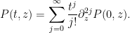
Now suppose we evolve 

On the space of polynomials of degree at most 
For instance, if one starts with a quadratic 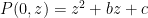

As the polynomial 

For instance, in the quadratic case, the quadratic formula tells us that the zeroes are

and
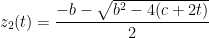
after arbitrarily choosing a branch of the square root. If 


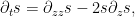
In the general case, we can obtain the equations of motion by implicitly differentiating the defining equation

in time using (2) to obtain

To simplify notation we drop the explicit dependence on time, thus

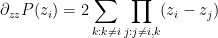
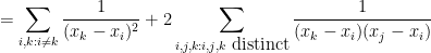
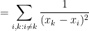
From (1) and the product rule, we see that

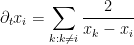
and
(where all indices are understood to range over 

at least when one avoids those times in which there is a repeated zero. In the case when the zeroes 


One interesting consequence of these equations is that if the zeroes are real at some time, then they will stay real as long as the zeroes do not collide. Let us now restrict attention to the case of real simple zeroes, in which case we will rename the zeroes as 

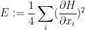
can now be thought of as reverse gradient flow for the “entropy”

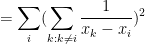
(which is also essentially the logarithm of the discriminant of the polynomial) since we have

In particular, we have the monotonicity formula

where 
where in the last line we use the antisymmetrisation identity

Among other things, this shows that as one goes backwards in time, the entropy decreases, and so no collisions can occur to the past, only in the future, which is of course consistent with the attractive nature of the dynamics. As 

Exercise 1 Show that

Symmetric polynomials of the zeroes are polynomial functions of the coefficients and should thus evolve in a polynomial fashion. One can compute this explicitly in simple cases. For instance, the center of mass is an invariant:

The variance decreases linearly:
Exercise 2 Establish the virial identity
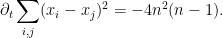
As the variance (which is proportional to 

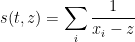
Exercise 3 Show that the Stieltjes transform
solves the viscous Burgers equation
either by using the original heat equation (2) and the identity
, or else by using the equations of motion (3). This relation between the Burgers equation and the heat equation is known as the Cole-Hopf transformation.
The paper of Csordas, Smith, and Varga mentioned previously gives some other bounds on the lifespan of the dynamics; roughly speaking, they show that if there is one pair of zeroes that are much closer to each other than to the other zeroes then they must collide in a short amount of time (unless there is a collision occuring even earlier at some other location). Their argument extends also to situations where there are an infinite number of zeroes, which they apply to get new results on Newman’s conjecture in analytic number theory. I would be curious to know of further places in the literature where this dynamics has been studied.

40 comments
Comments feed for this article
17 October, 2017 at 7:30 pm
Anonymous
The equations of motion of point vortices (which solve the 2d Euler equations) satisfy an equation similar to your (3). See equation (6) of Aref’s Annual Review on vortex dipoles:
http://www.annualreviews.org/doi/pdf/10.1146/annurev.fl.15.010183.002021
20 October, 2017 at 5:05 am
MatjazG
It looks very similar indeed, except for a rotation of each velocity by 90° (in the complex plane) and complex conjugation. Namely, the vortices tend to swirl around one another, not collide as the polynomial zeros tend to do under heat flow. In fact, the motion of vortices is described by a Hamiltonian dynamical system (for equal strength vortices
  is the generalized position and
  is the generalized momentum) where the conserved Hamiltonian is, for equal strength vortices, precisely the entropy defined for the heat flow
  . This immediately shows that point 2D vortices can in fact never collide.
We can get a bit closer to vortex motion if we Wick rotate (meaning we replace with
with  , i.e., we evolve “in complex time”) the heat Eq. (2) into the Schrödinger equation:
  . Then the Wick rotated solution for the polynomial zeroes Eq. (3) acquires an extra
  which is needed to rotate the velocity
  by 90° in the complex plane. The “only” thing that is missing is complex conjugation of the velocity (i.e. reflection across the real line).
This missing complex conjugation is quite important, however, as at least my numerical simulations tend to show that the polynomial zeroes now mostly repel one another and at late times quickly approach pair-wise diverging motion along the directions (I checked for up to 4th order polynomials), but do not seem to ever collide at least in generic cases (there are fine-tuned degenerate cases like the
  polynomial, though, where they do collide, and cases like polynomials of order 3 where a pair of zeroes diverges along
  but one zero remains near the origin). The behaviour is similar to dynamical-system motion around a hyperbolic point instead of an elliptical one as for the motion of point vortices.
At present I do not see a trivial deformation of the heat/Schrödinger equation that would give the motion of polynomial zeros that is the same as the motion of point vortices (complex conjugating P on one side of the heat/Schrödinger equation does not do it, of course). It is intriguing how close it seems, though.
20 October, 2017 at 8:23 am
hxypqr
yeah,i just do a similar calculate and get the same dynamic picture in my mind,but i do not think the whole story in a physics picture.anyway,one key obeserve is that the points should diverging along n distinct line to infinity in the complex plane .at least in the case the limit polynomial has n distinct root.for the degenerate situation the thing is not so easy to control we need to analysis to certain entanglement pairs.and if
  is odd,then we will have a root 0 in the limit case,this is also a annoying thing.
 ,this will corresponding to 2 different dynamic picture,because we do not know what happen at (0,0).this is a broken of symmetry.we need to use buried group and the jordan curve theorem(the topology only change when two point collide) to find the loss information.by the way,i think consider the deformation of zeros for polynomial function under heat equation on compact complex analytic surface(especially on
  ) is also interesting.
in my opinion,i think we need some knowledge from buried group to investigate a fix dynamic system generat by the zero of polynomial under heat flow,just think with the situation for quadratic polynomial
17 October, 2017 at 7:38 pm
Matt Karrmann
Hello Mr. Tao,
You appear to have confused the “fundamental theorem of arithmetic” with the “fundamental theorem of algebra” at the very beginning of this post.
I would like you to know that I am truly honored to have the opportunity to point this out to you. Great post otherwise and I really appreciate the fact that you put these posts out!
P.S. In case the tone is unclear over text, I’m not pointing this out in a demeaning manner or even out of serious concern. I simply never thought I’d ever catch one of your mistakes, and I found so ironic that THIS was the mistake, that I simply had to say something! Once again, I really appreciate the fact that you make these posts!
[Corrected, thanks – T.]
18 October, 2017 at 2:43 am
Tapash Bhagabati
I totally agree with you.
Geniuses make mistakes too (Though it is a unintentional) !
18 October, 2017 at 6:11 am
Anonymous
It is a typo, no confusion.
17 October, 2017 at 7:42 pm
André Camargo
I believe there is a typo in the series expansion of $P(t,z)$. Apparently the The right-hand side of the equation just after (2) does not depend on $t$.
[Corrected, thanks – T.]
17 October, 2017 at 8:05 pm
Matt Karrmann
Instead of “1” on the RHS, it should be $t^n$.
[Corrected, thanks – T.]
17 October, 2017 at 10:06 pm
Theodore Kolokolnikov
This resembles the classical Helmholtz equations for motion of fluid vortices in the plane. I wonder what the wave equation gives…
18 October, 2017 at 3:10 am
Anonymous
If is (locally) analytic in
  , it has (locally) the same zero set as its Weierstrass polynomial (in
  – with analytic coefficients in
  ) – so the (local) dynamics of the zeros can be represented by their Puiseux series. Is it possible to extend (locally) the above results for (possibly infinitely many) zeros arranged in separated clusters of (possibly colliding) zeros?
18 October, 2017 at 7:00 am
arch1
Beginner Q: Is it implicit in (2) that also P(0,z) = P(z)? Otherwise (2) does not seem to establish a relationship between P(t,z) and P(z).
[This implicit equivalence has now been added – T.]
18 October, 2017 at 9:57 am
Anonymous
Treating it as an optimal transport problem, I wonder if the behavior of the zeroes is a consequence of the relationship between energy geodesics, entropy and the manifold curvature (as treated for other dynamics by, for example, Cedric Villani in his “lazy gas experiment”).
18 October, 2017 at 11:20 am
Anonymous
Numerical examples here: https://twitter.com/gabrielpeyre/status/920731190461648896
18 October, 2017 at 12:26 pm
Paul Bristol
Fundamental theorem of algebra of course, not arithmetic.
[Corrected, thanks – T.]
18 October, 2017 at 1:55 pm
Frank Murphy
Reblogged this on fmurphyrng.
18 October, 2017 at 3:46 pm
Sujit Nair
Dimensions are incorrect in the Taylor series for [math]P(t,z)[/math]. The right side needs [math]t^n[/math] inside the summation.
[Corrected, thanks – T.]
19 October, 2017 at 11:38 am
hxypqr
Dear terry tao:
I think the limit case of the dynamic system is under control,I just mean we due to we can calculate the equation
exactly,so we can rescaling it and take $t\to \infty$,the limit case is the equation:
until now,at least for the case the n zero is distinct in (*),we know at last the zero will go to infinity along each direction come form the zeros of (*),so the only complicated thing is the finite “blow up”time i.e. the time zeroes must collide.these will lead to to breaken of symmetry(just think about the example
19 October, 2017 at 11:40 am
Heat flow and the zero of polynomial-a approach to Riemann Hypesis | Relationship of relationship
[…] this is a note after reading the blog:Heat flow and the zero of polynomial. […]
20 October, 2017 at 7:43 am
Aula
The letter n is used as both the degree of the polynomial and the summation index of the Taylor series. Perhaps a different letter could be used in the latter purpose to avoid any possible confusion.
[Summation index changed – T.]
21 October, 2017 at 3:35 am
MK
Your equation (3) reminds one of the dynamics of zeros of a power series when the coefficients undergo Brownian motions. The difference from Dyson’s BM is that the inverse distances to other zeros appears in the variance (not the drift) of the diffusion describing the motion of a particular root.
Here is (1) A movie: https://www.stat.berkeley.edu/~peres/GAF/dynamics/dynamics.html (2) Analysis by Peres and Virag: Display (49) of https://arxiv.org/pdf/math/0310297.pdf
22 October, 2017 at 11:39 pm
ustc liu
Does this have connection with Lee-Yang theorem about the zeros of partition function in statistical mechanics?
30 October, 2017 at 1:47 pm
BR
I am not an expert on the Lee-Yang theorem, but there is at least a small but interesting historical connection — see the (well written and self-contained) remarks made by Mark Kac at the end of the 3rd volume of Polya’s collected works, on Polya’s paper `Bemerkung uber die integraldarstellung der Riemannschen -funktion’.
26 October, 2017 at 12:17 pm
shannon7774
Solutions of the form for all k give the equations of Stieltjes for the optimizer of the Coulomb gas model as in Mehta appendix 6, whose solution is Hermite zeros in random matrix theory. This is obvious b/c the Coulomb gas model is H plus the sum-of-squares. But it is also the self-similar solution of the dynamics.
11 November, 2017 at 6:28 pm
kjkj309
Thanks for the reference. What is the motivation for the sum-of-squares term in that model?
10 November, 2017 at 6:05 am
C Trombley
Equation after “in time using (2) to obtain” should be a difference rather than a sum, no?
[No. -T]
11 November, 2017 at 12:47 pm
kjkj309
Does anyone have any insight on how one could come up with the sum-of-squares representation for in Exercise 1, if one did not know it in advance? How are these algebraic identities discovered by mathematicians in practice?
11 November, 2017 at 5:09 pm
Terence Tao
As I wrote in the post, this identity ultimately arises from the convexity of . If
. If  obeys (reverse) gradient flow
  , then
  . If
. If  is convex, then
  is positive definite and the RHS should be expressible as the sum of squares. If one pursues this line of reasoning a bit more, one will ultimately arrive at the identity in Exercise 1.
11 November, 2017 at 6:26 pm
kjkj309
Oh, nice! Thanks so much for your reply. I should have paid more attention to the sentence about convexity in the post.
19 January, 2018 at 4:21 am
The De Bruijn-Newman constant is non-negativ | What's new
[…] the argument proceeds as follows. As observed by Csordas, Smith, and Vargas (and also discussed in this previous blog post, the backwards heat evolution of the introduces a nice ODE dynamics on the zeroes of , namely […]
7 June, 2018 at 3:15 am
Heat flow and zeroes of polynomials II: zeroes on a circle | What's new
[…] is a sequel to this previous blog post, in which we discussed the effect of the heat flow […]
1 July, 2018 at 4:34 am
Maths student
Dear Prof. Tao, dear readers,
I was just interested in the following: Let’s say we’ve got a random matrix. We can associate to it a monic polynomial by taking the characteristic polynomial, and then develop it with the heat equation (or any other equation). Then all the quantities above become random variables, dependent on the entries of the random matrix.
Are these of any interest? They seem to correspond to a “real-world” problem: Namely, when the initial data is random, what can we expect after some time? (Of course only when one is interested in what the zeroes of the respective function do.)
2 July, 2018 at 7:05 am
Terence Tao
It seems that random matrices and heat flows inhabit parallel, but disconnected, “worlds”, parameterised by an inverse temperature parameter , and that it is not particularly natural to mix the different worlds together. Heat flow corresponds to the deterministic (
 ) world, being connected in particular to the finite free convolution of Marcus, Spielman, and Srivastava. The random matrices relating to the Gaussian Unitary Ensemble instead lie in the
  world, the random matrices relating to the Gaussian Orthogonal Ensemble lie in the
  world, and so forth. Each
  has its own flow; for
  it would be the Dyson Brownian motion, which looks nearly identical to the heat flow dynamics of zeroes but with an additional Brownian drift term, and corresponds to perturbing each entry of the matrix by a (complex) Gaussian perturbation (subject to maintaining the Hermitian property).
3 July, 2018 at 12:22 pm
Maths student
Thanks a lot! (Even though it’s slightly frustrating being illustrated the inferiority of one’s intellectual abilities by a peer just rattling off fringe theories fitting the subject squarely that go a thousand miles beyond showing that the statistics are just not interesting…)
28 April, 2022 at 12:24 pm
Brian C. Hall
Dear Maths student, please see my post below about a random matrix interpretation of the heat flow.
22 March, 2019 at 1:59 pm
Dynamical Phase Portraits | Empathic Dynamics
[…] while ago Terence Tao wrote a post about the heat flow of polynomials, whereby one can think of a family of polynomials in a variable , and consider what happens to them […]
28 April, 2022 at 12:23 pm
Brian C. Hall
A recent preprint of mine with Ching-Wei Ho gives a random matrix interpretation to the evolution of the zeros of polynomials under the heat flow, but only if you go past the first collision time and allow the roots to become complex. As a special case, we conjecture that if you apply the heat operator for time 1/N to the characteristic polynomial of an NxN GUE matrix, the roots of the new polynomial will be asymptotically uniform on the unit disk. That is, the heat flow changes semicircular to circular. See: https://arxiv.org/abs/2202.09660
3 July, 2022 at 2:17 pm
Anonymous
If $\xi$ has only simple zeros then RH is true?
3 July, 2022 at 11:22 pm
Terence Tao
No; technically, they are logically independent statements. However, the combination of the Riemann Hypothesis and the Simple Zeroes Conjecture turns out to be a natural strengthening of the RH alone in some cases; see this MathOverflow post for further discussion.
12 July, 2022 at 5:33 am
Heat flow and the zero of polynomial-a approach to Riemann Hypesis - Relationship of relationship
[…] this is a note after reading the blog:Heat flow and the zero of polynomial. […]
17 October, 2023 at 8:57 am
Anonymous
Hi. I had done a similar study with the help of canonical representations of geometric objects in 2- and 3-dimensional space. This has become more clear in my mind with your work. Maybe there is a relationship between stationary points of flow and roots.