In this post we assume the Riemann hypothesis and the simplicity of zeroes, thus the zeroes of  in the critical strip take the form
  for some real number ordinates
  . From the Riemann-von Mangoldt formula, one has the asymptotic
as  ; in particular, the spacing
  should behave like
  on the average. However, it can happen that some gaps are unusually small compared to other nearby gaps. For the sake of concreteness, let us define a Lehmer pair to be a pair of adjacent ordinates
  such that
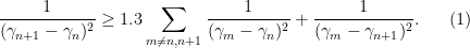
The specific value of constant  is not particularly important here; anything larger than
  would suffice. An example of such a pair would be the classical pair


discovered by Lehmer. It follows easily from the main results of Csordas, Smith, and Varga that if an infinite number of Lehmer pairs (in the above sense) existed, then the de Bruijn-Newman constant  is non-negative. This implication is now redundant in view of the unconditional results of this recent paper of Rodgers and myself; however, the question of whether an infinite number of Lehmer pairs exist remain open.
In this post, I sketch an argument that Brad and I came up with (as initially suggested by Odlyzko) the GUE hypothesis implies the existence of infinitely many Lehmer pairs. We argue probabilistically: pick a sufficiently large number  , pick
  at random from
  to
to  (so that the average gap size is close to
  ), and prove that the Lehmer pair condition (1) occurs with positive probability.
Introduce the renormalised ordinates  for
for  , and let
  be a small absolute constant (independent of ). It will then suffice to show that

![\displaystyle 1.3 \sum_{m \in [T \log T, 2T \log T]: m \neq n,n+1} \frac{1}{(x_m - x_n)^2} + \frac{1}{(x_m - x_{n+1})^2}](https://s0.wp.com/latex.php?latex=%5Cdisplaystyle+1.3+%5Csum_%7Bm+%5Cin+%5BT+%5Clog+T%2C+2T+%5Clog+T%5D%3A+m+%5Cneq+n%2Cn%2B1%7D+%5Cfrac%7B1%7D%7B%28x_m+-+x_n%29%5E2%7D+%2B+%5Cfrac%7B1%7D%7B%28x_m+-+x_%7Bn%2B1%7D%29%5E2%7D&bg=ffffff&fg=000000&s=0&c=20201002)

(say) with probability  , since the contribution of those
  outside of
 ![{[T \log T, 2T \log T]}](https://s0.wp.com/latex.php?latex=%7B%5BT+%5Clog+T%2C+2T+%5Clog+T%5D%7D&bg=ffffff&fg=000000&s=0&c=20201002) can be absorbed by the
can be absorbed by the  factor with probability
  .
.
As one consequence of the GUE hypothesis, we have  with probability
  . Thus, if
 ![{E := \{ m \in [T \log T, 2T \log T]: x_{m+1} - x_m \leq \varepsilon^2 \}}](https://s0.wp.com/latex.php?latex=%7BE+%3A%3D+%5C%7B+m+%5Cin+%5BT+%5Clog+T%2C+2T+%5Clog+T%5D%3A+x_%7Bm%2B1%7D+-+x_m+%5Cleq+%5Cvarepsilon%5E2+%5C%7D%7D&bg=ffffff&fg=000000&s=0&c=20201002) , then
, then  has density
  . Applying the Hardy-Littlewood maximal inequality, we see that with probability , we have
![\displaystyle \sup_{h \geq 1} | \# E \cap [n+h, n-h] | \leq \frac{1}{10}](https://s0.wp.com/latex.php?latex=%5Cdisplaystyle++%5Csup_%7Bh+%5Cgeq+1%7D+%7C+%5C%23+E+%5Ccap+%5Bn%2Bh%2C+n-h%5D+%7C+%5Cleq+%5Cfrac%7B1%7D%7B10%7D+&bg=ffffff&fg=000000&s=0&c=20201002)
which implies in particular that

for all ![{m \in [T \log T, 2 T \log T] \backslash \{ n, n+1\}}](https://s0.wp.com/latex.php?latex=%7Bm+%5Cin+%5BT+%5Clog+T%2C+2+T+%5Clog+T%5D+%5Cbackslash+%5C%7B+n%2C+n%2B1%5C%7D%7D&bg=ffffff&fg=000000&s=0&c=20201002) . This implies in particular that
. This implies in particular that
![\displaystyle \sum_{m \in [T \log T, 2T \log T]: |m-n| \geq \varepsilon^{-3}} \frac{1}{(x_m - x_n)^2} + \frac{1}{(x_m - x_{n+1})^2} \ll \varepsilon^{-1}](https://s0.wp.com/latex.php?latex=%5Cdisplaystyle++%5Csum_%7Bm+%5Cin+%5BT+%5Clog+T%2C+2T+%5Clog+T%5D%3A+%7Cm-n%7C+%5Cgeq+%5Cvarepsilon%5E%7B-3%7D%7D+%5Cfrac%7B1%7D%7B%28x_m+-+x_n%29%5E2%7D+%2B+%5Cfrac%7B1%7D%7B%28x_m+-+x_%7Bn%2B1%7D%29%5E2%7D+%5Cll+%5Cvarepsilon%5E%7B-1%7D+&bg=ffffff&fg=000000&s=0&c=20201002)
and so it will suffice to show that

![\displaystyle \geq 1.3 \sum_{m \in [T \log T, 2T \log T]: m \neq n,n+1; |m-n| < \varepsilon^{-3}} \frac{1}{(x_m - x_n)^2} + \frac{1}{(x_m - x_{n+1})^2} + \frac{1}{5\varepsilon^2}](https://s0.wp.com/latex.php?latex=%5Cdisplaystyle+%5Cgeq+1.3+%5Csum_%7Bm+%5Cin+%5BT+%5Clog+T%2C+2T+%5Clog+T%5D%3A+m+%5Cneq+n%2Cn%2B1%3B+%7Cm-n%7C+%3C+%5Cvarepsilon%5E%7B-3%7D%7D+%5Cfrac%7B1%7D%7B%28x_m+-+x_n%29%5E2%7D+%2B+%5Cfrac%7B1%7D%7B%28x_m+-+x_%7Bn%2B1%7D%29%5E2%7D+%2B+%5Cfrac%7B1%7D%7B5%5Cvarepsilon%5E2%7D&bg=ffffff&fg=000000&s=0&c=20201002)
(say) with probability .
By the GUE hypothesis (and the fact that  is independent of ), it suffices to show that a Dyson sine process
  , normalised so that
  is the first positive point in the process, obeys the inequality

with probability  . However, if we let
  be a moderately large constant (and assume small depending on
  ), one can show using
  -point correlation functions for the Dyson sine process (and the fact that the Dyson kernel
  equals
  to second order at the origin) that
![\displaystyle {\bf E} N_{[-\varepsilon,0]} N_{[0,\varepsilon]} \gg \varepsilon^4](https://s0.wp.com/latex.php?latex=%5Cdisplaystyle++%7B%5Cbf+E%7D+N_%7B%5B-%5Cvarepsilon%2C0%5D%7D+N_%7B%5B0%2C%5Cvarepsilon%5D%7D+%5Cgg+%5Cvarepsilon%5E4+&bg=ffffff&fg=000000&s=0&c=20201002)
![\displaystyle {\bf E} N_{[-\varepsilon,0]} \binom{N_{[0,\varepsilon]}}{2} \ll \varepsilon^7](https://s0.wp.com/latex.php?latex=%5Cdisplaystyle++%7B%5Cbf+E%7D+N_%7B%5B-%5Cvarepsilon%2C0%5D%7D+%5Cbinom%7BN_%7B%5B0%2C%5Cvarepsilon%5D%7D%7D%7B2%7D+%5Cll+%5Cvarepsilon%5E7+&bg=ffffff&fg=000000&s=0&c=20201002)
![\displaystyle {\bf E} \binom{N_{[-\varepsilon,0]}}{2} N_{[0,\varepsilon]} \ll \varepsilon^7](https://s0.wp.com/latex.php?latex=%5Cdisplaystyle++%7B%5Cbf+E%7D+%5Cbinom%7BN_%7B%5B-%5Cvarepsilon%2C0%5D%7D%7D%7B2%7D+N_%7B%5B0%2C%5Cvarepsilon%5D%7D+%5Cll+%5Cvarepsilon%5E7+&bg=ffffff&fg=000000&s=0&c=20201002)
![\displaystyle {\bf E} N_{[-\varepsilon,0]} N_{[0,\varepsilon]} N_{[\varepsilon,A^{-1}]} \ll A^{-3} \varepsilon^4](https://s0.wp.com/latex.php?latex=%5Cdisplaystyle++%7B%5Cbf+E%7D+N_%7B%5B-%5Cvarepsilon%2C0%5D%7D+N_%7B%5B0%2C%5Cvarepsilon%5D%7D+N_%7B%5B%5Cvarepsilon%2CA%5E%7B-1%7D%5D%7D+%5Cll+A%5E%7B-3%7D+%5Cvarepsilon%5E4+&bg=ffffff&fg=000000&s=0&c=20201002)
![\displaystyle {\bf E} N_{[-\varepsilon,0]} N_{[0,\varepsilon]} N_{[-A^{-1}, -\varepsilon]} \ll A^{-3} \varepsilon^4](https://s0.wp.com/latex.php?latex=%5Cdisplaystyle++%7B%5Cbf+E%7D+N_%7B%5B-%5Cvarepsilon%2C0%5D%7D+N_%7B%5B0%2C%5Cvarepsilon%5D%7D+N_%7B%5B-A%5E%7B-1%7D%2C+-%5Cvarepsilon%5D%7D+%5Cll+A%5E%7B-3%7D+%5Cvarepsilon%5E4+&bg=ffffff&fg=000000&s=0&c=20201002)
![\displaystyle {\bf E} N_{[-\varepsilon,0]} N_{[0,\varepsilon]} N_{[-k, k]}^2 \ll k^2 \varepsilon^4 \ \ \ \ \ (3)](https://s0.wp.com/latex.php?latex=%5Cdisplaystyle++%7B%5Cbf+E%7D+N_%7B%5B-%5Cvarepsilon%2C0%5D%7D+N_%7B%5B0%2C%5Cvarepsilon%5D%7D+N_%7B%5B-k%2C+k%5D%7D%5E2+%5Cll+k%5E2+%5Cvarepsilon%5E4+%5C+%5C+%5C+%5C+%5C+%283%29&bg=ffffff&fg=000000&s=0&c=20201002)
for any natural number , where  denotes the number of elements of the process in
  . For instance, the expression
 ![{{\bf E} N_{[-\varepsilon,0]} \binom{N_{[0,\varepsilon]}}{2} }](https://s0.wp.com/latex.php?latex=%7B%7B%5Cbf+E%7D+N_%7B%5B-%5Cvarepsilon%2C0%5D%7D+%5Cbinom%7BN_%7B%5B0%2C%5Cvarepsilon%5D%7D%7D%7B2%7D+%7D&bg=ffffff&fg=000000&s=0&c=20201002) can be written in terms of the three-point correlation function
can be written in terms of the three-point correlation function  as
as

which can easily be estimated to be  (since
  in this region), and similarly for the other estimates claimed above.
Since for natural numbers  , the quantity
  is only positive when
  , we see from the first three estimates that the event that
 ![{N_{[-\varepsilon,0]} = N_{[0,\varepsilon]} = 1}](https://s0.wp.com/latex.php?latex=%7BN_%7B%5B-%5Cvarepsilon%2C0%5D%7D+%3D+N_%7B%5B0%2C%5Cvarepsilon%5D%7D+%3D+1%7D&bg=ffffff&fg=000000&s=0&c=20201002) occurs with probability . In particular, by Markov’s inequality we have the conditional probabilities
occurs with probability . In particular, by Markov’s inequality we have the conditional probabilities
![\displaystyle {\bf P} ( N_{[\varepsilon,A^{-1}]} \geq 1 | E ) \ll A^{-3}](https://s0.wp.com/latex.php?latex=%5Cdisplaystyle++%7B%5Cbf+P%7D+%28+N_%7B%5B%5Cvarepsilon%2CA%5E%7B-1%7D%5D%7D+%5Cgeq+1+%7C+E+%29+%5Cll+A%5E%7B-3%7D+&bg=ffffff&fg=000000&s=0&c=20201002)
![\displaystyle {\bf P} ( N_{[-A^{-1}, -\varepsilon]} \geq 1 | E ) \ll A^{-3}](https://s0.wp.com/latex.php?latex=%5Cdisplaystyle++%7B%5Cbf+P%7D+%28+N_%7B%5B-A%5E%7B-1%7D%2C+-%5Cvarepsilon%5D%7D+%5Cgeq+1+%7C+E+%29+%5Cll+A%5E%7B-3%7D+&bg=ffffff&fg=000000&s=0&c=20201002)
![\displaystyle {\bf P} ( N_{[-k, k]} \geq A k^{5/3} | E ) \ll A^{-4} k^{-4/3}](https://s0.wp.com/latex.php?latex=%5Cdisplaystyle++%7B%5Cbf+P%7D+%28+N_%7B%5B-k%2C+k%5D%7D+%5Cgeq+A+k%5E%7B5%2F3%7D+%7C+E+%29+%5Cll+A%5E%7B-4%7D+k%5E%7B-4%2F3%7D+&bg=ffffff&fg=000000&s=0&c=20201002)
and thus, if is large enough, and small enough, it will be true with probability that
![\displaystyle N_{[-\varepsilon,0]}, N_{[0,\varepsilon]} = 1](https://s0.wp.com/latex.php?latex=%5Cdisplaystyle++N_%7B%5B-%5Cvarepsilon%2C0%5D%7D%2C+N_%7B%5B0%2C%5Cvarepsilon%5D%7D+%3D+1&bg=ffffff&fg=000000&s=0&c=20201002)
and
![\displaystyle N_{[A^{-1}, \varepsilon]} = N_{[\varepsilon, A^{-1}]} = 0](https://s0.wp.com/latex.php?latex=%5Cdisplaystyle++N_%7B%5BA%5E%7B-1%7D%2C+%5Cvarepsilon%5D%7D+%3D+N_%7B%5B%5Cvarepsilon%2C+A%5E%7B-1%7D%5D%7D+%3D+0&bg=ffffff&fg=000000&s=0&c=20201002)
and simultaneously that
![\displaystyle N_{[-k,k]} \leq A k^{5/3}](https://s0.wp.com/latex.php?latex=%5Cdisplaystyle++N_%7B%5B-k%2Ck%5D%7D+%5Cleq+A+k%5E%7B5%2F3%7D&bg=ffffff&fg=000000&s=0&c=20201002)
for all natural numbers . This implies in particular that

and

for all  , which gives (2) for small enough.
Remark 1 The above argument needed the GUE hypothesis for correlations up to fourth order (in order to establish (3)). It might be possible to reduce the number of correlations needed, but I do not see how to obtain the claim just using pair correlations only.


28 comments
Comments feed for this article
20 January, 2018 at 12:41 pm
zgtzsj
The link to Riemann-von Mangoldt formula seems not correct. Should be this one: https://en.wikipedia.org/wiki/Riemann%E2%80%93von_Mangoldt_formula
[Corrected, thanks – T.]
23 January, 2018 at 7:13 am
zgtzsj
seems that you still haven’t changed it. It is: https://en.wikipedia.org/wiki/Riemann%E2%80%93von_Mangoldt_formula
[Should be OK now – T.]
20 January, 2018 at 11:05 pm
Aula
In (1) the constant is 1.3 but in all later appearances it is 1.4. Also, there are two displays that are too wide to be shown completely; the second one is obvious because it cuts off in the middle of a fraction, but the first one looks fine until you start to wonder why it doesn’t have the error term mentioned in the text.
[Corrected, thanks -T.]
21 January, 2018 at 12:09 pm
Brian Tennesob
Hello professor Tao,
My name is Brian.
I only have a masters in math so I do not have a PhD. I can follow your arguments to some extent but as I have only taken a few analysis courses, I don’t fully comprehend everything here.
I was wondering how can I get up to speed on the Riemann hypothesis which seems that if it is true then it is only “barely so” as you explaned previously.
Do you think that is why it’s resolution has been so elusive over the years?
Also, I have another question and I hope it doesn’t appear as naive as I think it might sound to you.
I am very interested in automated theorem proving. There are many difficulties with ATP’s and proof assistants and the like. However with breakthroughs in machine learning, there has been some (but not much) discussion about applying machine learning to automated theorem provers, mainly in the heurisitcs of how the computer attempts to approach the proof.
Of course one extremely important problem is correctly formalizing the RH into a way the would avail itself to even begin the process of conducting a search for a proof of RH or the negation of RH, whatever the case may be. Also, even the best ATP might take longer than the age of the universe to decide RH or not RH. And, on top of all that, the proof or disproof of RH might be a proof that is so long that it takes petabytes upon petabytes to store in machine level formalized proof.
So from what little I know of analysis and automated theorem proving, deciding RH, even with the best heuristics and software, its proof may be literally impossible for even the smartest humans to ever check.
This kind of solution to RH would thus be extremely unsatisfying to me and probably everyone else who is involved in RH. And if no one can fully check the proof or disproof of RH, we humans will perhaps gain nothing at all from a formal proof that is petabytes in length, if it is even that small!
Do you think I should go for a PhD in an analysis-related field for RH, number theory, or (and this is going to sound dreadful) computer science?
Finally, if I did get so far as to have an ATP decide the RH, would I be eligible for the Clay institute’s $1,000,000 prize if my ATP’s proof is so long that no human can check it?
I hope this is the right place to ask due to the subject of the last two of your posts connected to the zeta function, though admittedly I am not asking about this post directly.
I appreciate your time. Though I don’t fully understand your post, I know just enough about writing proofs to be able to see that each and every one of your posts is literally a masters class in how to write sharp and elegant proofs, something that is way off from a brute force computer search for a decision on RH which, I am certain, would leave everyone quite unsatisfied to say the least!
In fact, even if my computer decided RH, I would not be very satisfied with such an inelegant proof!
Any thoughts at all that you might have would be immensely appreciated professor Tao and if you would be so kind as to provide me guidance by providing good references on RH or automated heorem proving, I would forever be in your debt.
Thanks, Brian
3 April, 2018 at 1:19 am
Anonymous
Lot of downvotes, because a little bit of rambling, but the question is quite clear, I think, and fair:
Go with whatever you would go, if there was no Riemann Hypothesis. If you love math, then study pure math.
If your computer code, which eventually yields the RH, is very clear and bullet proof, then this will be a proof of the RH, and you will have proven the RH. And then get the price. The price doesn’t say anything about HOW you should proof it. A proof is a proof.
Now, whether your code will be a proof, it depends on the specific code. People don’t need to understand the write-up of the proof, if they can believe that the code checked it correctly.
Finally, there is no reason to believe that deep learning can prove anything (noteworthy). If you use classical approaches, where do you find the data which form the basis? Deep Learning in its classic form is only good at producing quickly a result, which a human with some time could produce himself.
Now, you could think about Reinforcement Learning, where you set up the reward function in such a way that you move towards the RH, but … , I dont see how…
21 January, 2018 at 12:33 pm
tennesb
Reblogged this on briantenneson.
21 January, 2018 at 4:06 pm
Joseph
I think that 3-correlations are sufficient: we can remove the square in (3), getting a bound with instead of
  . We can then deduce in the same way, with large conditional probability given
  , the bound
 ![N_{[-k,k]} \leq A k ^{5/3}](https://s0.wp.com/latex.php?latex=N_%7B%5B-k%2Ck%5D%7D+%5Cleq+A+k+%5E%7B5%2F3%7D&bg=ffffff&fg=545454&s=0&c=20201002) for
for  equal to (say) a power of two. This gives
 ![N_{[-k,k]} \leq A (2k)^{5/3}](https://s0.wp.com/latex.php?latex=N_%7B%5B-k%2Ck%5D%7D+%5Cleq+A+%282k%29%5E%7B5%2F3%7D&bg=ffffff&fg=545454&s=0&c=20201002) for all integers
for all integers  .
.
However, my guess would be that the pair correlations are not enough: it seems to me that one can respect these correlations with a point process such that small gaps come by groups of two.
21 January, 2018 at 9:29 pm
Terence Tao
Nice! I forgot about the trick of sparsifying the to be dyadic (also the key trick in proving the strong law of large numbers). I think find your argument that pair correlations are not sufficient to be plausible, though I don’t know how to actually construct such a process as you describe…
22 January, 2018 at 1:14 pm
BR
To go at somewhat of a tangent, a related question is whether one can even write down a translation invariant point process with 1 and 2 level correlations mimicking the sine process but which is not actually the sine-process? (Leaving aside for the moment whether you can force small gaps to come in pairs.) That is, does there exist a translation invariant point process with configurations such that
which is not the sine process? I think almost certainly there exist processes of this sort, but constructing one seems difficult… Note that such a point process can’t be determinantal.
21 January, 2018 at 10:26 pm
Anonymous
Since an infinite number of Lehmer pairs (which now seems likely) imply that RH almost fails infinitely often, assuming RH is true, it means there is likely some deeper structure which prevents that from happening every time.
One relatively simpler but not rigorous argument seems to come from Riemann von Mangoldt formula. If there is a zero off the critical line, it would need an infinite number of counterparts on the same “off-line”, since a finite number of large oscillations would make the prime number distribution chaotic in small intervals. Also Ingham style results show that non-critical line zeroes have low density, which makes it even more difficult to have a complete off-line with infinite number of zeroes.
But it’s likely this structural constraint is already suspected. Is there a notion of a deeper constraint than this?
This situation seems analogous to Fermat’s last theorem where there are many near misses, but I think Wiles’ proof shows a strong geometric restriction and hence a structure against those.
22 January, 2018 at 12:05 am
Anonymous
It think that a finite number of “large oscillations” (caused by a finite set of zeros attaining the supremum over the zeros real parts – which, in such a case, should be < 1) would make the primes distribution less chaotic asymptotically (with a much better finite series approximation in the PNT theorem). The observed chaotic behavior of the primes distribution over short intervals, seems to indicate that if the supremum of the zeros real parts is attained, it must be attained by infinitely many zeros.
22 January, 2018 at 8:37 am
Anonymous
Well by chaotic behaviour in the RvM formula, I meant both large positive and negative deviations (greater than sqrt(x)) from the average x estimate occuring in a short range (x,x+h) where h could even be as low as 2 (such sharp reversals are of course not observed in reality). With a finite number of zeroes with large real parts, asymptotically the critical line zeroes will become irrelevant in RvM, and such reversals will occur infinitely often.
22 January, 2018 at 8:43 am
Anonymous
The last line may need further elaboration. With an infinite number of zeroes with large supremum real part, such reversals can be mitigated. But the likelihood of having such a line is quite low.
22 January, 2018 at 2:08 pm
Terence Tao
My vague feeling on this is that even though zeroes of the zeta function can occasionally be close to each other, there is a “repulsion” effect that keeps them from colliding off of the critical line and into the rest of the complex plane. Unfortunately, given the lack of dynamics in zeta (in particular, the lack of any time-like parameter one can vary), I can’t see any way to rigorously describe this repulsion. But it certainly exists in the random matrix models, see e.g. my previous blog post https://terrytao.wordpress.com/2008/10/28/when-are-eigenvalues-stable/ (or observe the repulsion term in the equations for Dyson Brownian motion). There is also the old Polya-Hilbert dream of somehow interpreting the zeroes of zeta as (a suitable renormalisation of) the eigenvalues of a self-adjoint operator, so that the self-adjointness would supply the constraint that keeps the zeroes on the critical line, even though they could still be permitted to approach each other. Perhaps one should proceed first by improving our understanding of the function field Riemann Hypothesis, which is actually a theorem…
24 January, 2018 at 10:20 am
Anonymous
When it comes to transitioning results from function field settings to larger fields, there has been some great work going on recently, for eg. using perfectoid spaces for proving weight monodromy in p-adic fields, among other results. Do you think such ideas have potential for the more regular fields?
24 January, 2018 at 6:16 pm
Terence Tao
I am not all that familiar with perfectoids, but as a general rule, progress in the function field case has mostly served as an analogy or guide for what ought to be true in the number field case (and vice versa), but it is rare that a technique that was first developed in function field settings has transferred over to the number field setting (though the converse seems to be significantly easier to accomplish), because number fields don’t seem to have as much geometric structure as function fields (e.g. no analogue of the Frobenius automorphism). (There is the dream of the “field of one element” being able to supply such geometric structure to number fields, but this is still largely a dream at the present time.)
25 January, 2018 at 4:10 am
Anonymous
I found the link I was referring to
Click to access PerfectoidSpaces.pdf
The author mentions in the introduction, ‘aim of this paper is to establish a general framework for reducing certain problems about mixed
characteristic rings to problems about rings in characteristic p’, which I feel is quite exciting.
22 January, 2018 at 10:42 am
Craig
I’m a bit confused as to how you get your third summation to be bounded by . From the prior line, it looks like you should get
  — or a bound of
  . That would mess up the argument completely, since you’re trying to show that the overall sum is bounded by
  .
.
[Oops, the cutoff should have been at rather than
  ; should be fixed now. -T]
23 January, 2018 at 9:32 am
Jeffrey Stopple
I don’t recognize the notation ? (I get that the bold E is expected value.)
[As stated in the text, denotes the number of zeroes in the interval
  . -T.]
23 January, 2018 at 10:09 am
Craig
Okay — I’d like to track powers of \epsilon in the last bit, especially when it comes to A. In your treatment, it looks like you’re formally treating A and \epsilon as independent, but I’m not sure they are. If you want your probabilities to be \gg \epsilon^4, then for N_{[-k,k]} \leq A k^{5/3}, you need A \gg \epsilon^{-1}.
Now, you conclude from the latter that |x_m – x_0| \gg_A |m|^{3/5}. Let’s make the A-dependence explicit — |x_m – x_0| \gg A^{-3/5} |m|^{3/5} with probability \gg \epsilon^4 if A \gg \epsilon^{-1}, so really |x_m – x_0| \gg \epsilon^{3/5} |m|^{3/5}.
Then the LHS of (2) is \gg \epsilon^{-2}, and the RHS is \ll \epsilon^{-6/5}, and everything checks out.
Cool!
23 January, 2018 at 7:21 pm
Terence Tao
One does not need to take that large. As long as the conditional probabilities
 ![{\bf P}(N_{[\varepsilon, A^{-1}]} \geq 1 | E)](https://s0.wp.com/latex.php?latex=%7B%5Cbf+P%7D%28N_%7B%5B%5Cvarepsilon%2C+A%5E%7B-1%7D%5D%7D+%5Cgeq+1+%7C+E%29&bg=ffffff&fg=545454&s=0&c=20201002) ,
, ![{\bf P}(N_{[-A^{-1}, -\varepsilon]} \geq 1 | E)](https://s0.wp.com/latex.php?latex=%7B%5Cbf+P%7D%28N_%7B%5B-A%5E%7B-1%7D%2C+-%5Cvarepsilon%5D%7D+%5Cgeq+1+%7C+E%29&bg=ffffff&fg=545454&s=0&c=20201002) , and
, and ![{\bf P}(N_{[-k,k]} \geq A k^{5/3} | E)](https://s0.wp.com/latex.php?latex=%7B%5Cbf+P%7D%28N_%7B%5B-k%2Ck%5D%7D+%5Cgeq+A+k%5E%7B5%2F3%7D+%7C+E%29&bg=ffffff&fg=545454&s=0&c=20201002) (as
(as  ranges over the natural numbers) sum to less than (say)
  , then on at least half of the event
  (and thus on an event of absolute probability
  ), one will have all the required properties. (As noted above by Joseph, one can do better here by restricting
  to be a power of 2, which is all that is needed for the rest of the argument.)
23 January, 2018 at 10:13 am
Craig
Note specifically that you can’t make A too large, as that shrinks |x_m – x_0| and increases the RHS of (2).
Fortunately the bound is A \ll \epsilon^{5/3}, which is larger than you need for your probabilities to work out.
24 January, 2018 at 11:47 am
Sujit Nair
If is picked at random from
 ![[T\log T,2T \log T]](https://s0.wp.com/latex.php?latex=%5BT%5Clog+T%2C2T+%5Clog+T%5D&bg=ffffff&fg=545454&s=0&c=20201002) , then
, then  is in
is in ![[2\pi T, 4\pi T]](https://s0.wp.com/latex.php?latex=%5B2%5Cpi+T%2C+4%5Cpi+T%5D&bg=ffffff&fg=545454&s=0&c=20201002) .
.
Does this imply that something like Bertrand’s postulate also holds true for the Riemann zeros, i.e., there is always a zero in![[2\pi T, 4\pi T]](https://s0.wp.com/latex.php?latex=%5B2%5Cpi+T%2C+4%5Cpi+T%5D&bg=ffffff&fg=545454&s=0&c=20201002) ?
?
24 January, 2018 at 3:58 pm
Terence Tao
For large enough, certainly, but not for very small
  ; for instance, there is no non-trivial zero of height between zero and
  . (But presumably one has a Bertrand-like result once
  exceeds
  , which can probably be derived from effective versions of the Riemann-von Mangoldt formula, combined with some numerical verification for medium values of
  .)
.)
29 January, 2018 at 10:33 am
Gil Kalai
A question regarding the GUE analogy: I suppose you can apply the heat kernet to the set of eigenvalues of a random GUE matrix. Is there a nice way to describe the outcome as actual eigenvalues for some noisy version of the random matrix?
29 January, 2018 at 11:44 am
Terence Tao
Nice question! My immediate guess would be no – most ensembles of real numbers don’t have a good random matrix theory interpretation, especially if there isn’t any nice structure such as determinantal structure (and I’m pretty sure applying heat flow to the characteristic polynomial of GUE will not yield a determinantal point process). Even if a matrix model did exist, it would be hard to find – I think for instance that there are random matrix models for beta ensembles for the non-classical values , but they are not immediately obvious (nor do they resemble GUE, GOE, or GSE in the classical cases); see https://arxiv.org/abs/math-ph/0206043 .
29 January, 2018 at 10:32 pm
Gil Kalai
Many thanks for the answer. It might be the case that heat-kernel eigenvalues correspond not to the eigenvalues of a single noisy random version of the matrix but to the expectation (or something like it) of the eigenvalues over noisy versions of the random version. The simplest such gadget would be to take the expected eigenvalues of where
where  is the random GUE matrix,
  is an independent random GUE matrix,
  .
.
10 October, 2018 at 9:55 am
Watching Over the Zeroes | Gödel's Lost Letter and P=NP
[…] argument that the RH is false. In January of this year, Brad Rogers and Terence Tao turned up the heat on this connection by proving that the GUE conjecture entails the existence of infinitely many […]