Brad Rodgers and I have uploaded to the arXiv our paper “The De Bruijn-Newman constant is non-negative“. This paper affirms a conjecture of Newman regarding to the extent to which the Riemann hypothesis, if true, is only “barely so”. To describe the conjecture, let us begin with the Riemann xi function
where  is the Gamma function and
  is the Riemann zeta function. Initially, this function is only defined for
  , but, as was already known to Riemann, we can manipulate it into a form that extends to the entire complex plane as follows. Firstly, in view of the standard identity
  , we can write

and hence

By a rescaling, one may write

and similarly
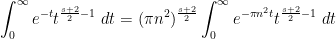
and thus (after applying Fubini’s theorem)
We’ll make the change of variables  to obtain

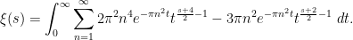
If we introduce the mild renormalisation

of  , we then conclude (at least for
  ) that
where  is the function

which one can verify to be rapidly decreasing both as  and as
  , with the decrease as faster than any exponential. In particular
  extends holomorphically to the upper half plane.
If we normalize the Fourier transform  of a (Schwartz) function
  as
as 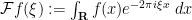 , it is well known that the Gaussian
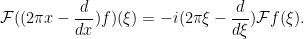
  is its own Fourier transform. The creation operator
  interacts with the Fourier transform by the identity
Since  , this implies that the function

is its own Fourier transform. (One can view the polynomial  as a renormalised version of the fourth Hermite polynomial.) Taking a suitable linear combination of this with , we conclude that

is also its own Fourier transform. Rescaling  by
by  and then multiplying by
  , we conclude that the Fourier transform of

is

and hence by the Poisson summation formula (using symmetry and vanishing at  to unfold the
  summation in (2) to the integers rather than the natural numbers) we obtain the functional equation
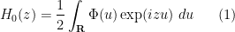
which implies that  and are even functions (in particular, now extends to an entire function). From this symmetry we can also rewrite (1) as
which now gives a convergent expression for the entire function  for all complex
  . As is even and real-valued on
  , is even and also obeys the functional equation
  , which is equivalent to the usual functional equation for the Riemann zeta function. The Riemann hypothesis is equivalent to the claim that all the zeroes of are real.
De Bruijn introduced the family  of deformations of
  , defined for all
  and
and  by the formula
From a PDE perspective, one can view  as the evolution of under the backwards heat equation
  . As with , the are all even entire functions that obey the functional equation
  , and one can ask an analogue of the Riemann hypothesis for each such , namely whether all the zeroes of are real. De Bruijn showed that these hypotheses were monotone in
  : if had all real zeroes for some , then
  would also have all zeroes real for any
  . Newman later sharpened this claim by showing the existence of a finite number
  , now known as the de Bruijn-Newman constant, with the property that had all zeroes real if and only if
  . Thus, the Riemann hypothesis is equivalent to the inequality
  . Newman then conjectured the complementary bound
  ; in his words, this conjecture asserted that if the Riemann hypothesis is true, then it is only “barely so”, in that the reality of all the zeroes is destroyed by applying heat flow for even an arbitrarily small amount of time. Over time, a significant amount of evidence was established in favour of this conjecture; most recently, in 2011, Saouter, Gourdon, and Demichel showed that
  .
.
In this paper we finish off the proof of Newman’s conjecture, that is we show that . The proof is by contradiction, assuming that  (which among other things, implies the truth of the Riemann hypothesis), and using the properties of backwards heat evolution to reach a contradiction.
Very roughly, the argument proceeds as follows. As observed by Csordas, Smith, and Varga (and also discussed in this previous blog post, the backwards heat evolution of the introduces a nice ODE dynamics on the zeroes  of , namely that they solve the ODE
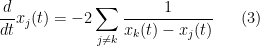
for all  (one has to interpret the sum in a principal value sense as it is not absolutely convergent, but let us ignore this technicality for the current discussion). Intuitively, this ODE is asserting that the zeroes repel each other, somewhat like positively charged particles (but note that the dynamics is first-order, as opposed to the second-order laws of Newtonian mechanics). Formally, a steady state (or equilibrium) of this dynamics is reached when the
  are arranged in an arithmetic progression. (Note for instance that for any positive
  , the functions
  obey the same backwards heat equation as , and their zeroes are on a fixed arithmetic progression
  .) The strategy is to then show that the dynamics from time
  to time
  creates a convergence to local equilibrium, in which the zeroes locally resemble an arithmetic progression at time
  . This will be in contradiction with known results on pair correlation of zeroes (or on related statistics, such as the fluctuations on gaps between zeroes), such as the results of Montgomery (actually for technical reasons it is slightly more convenient for us to use related results of Conrey, Ghosh, Goldston, Gonek, and Heath-Brown). Another way of thinking about this is that even very slight deviations from local equilibrium (such as a small number of gaps that are slightly smaller than the average spacing) will almost immediately lead to zeroes colliding with each other and leaving the real line as one evolves backwards in time (i.e., under the forward heat flow). This is a refinement of the strategy used in previous lower bounds on
  , in which “Lehmer pairs” (pairs of zeroes of the zeta function that were unusually close to each other) were used to limit the extent to which the evolution continued backwards in time while keeping all zeroes real.
How does one obtain this convergence to local equilibrium? We proceed by broad analogy with the “local relaxation flow” method of Erdos, Schlein, and Yau in random matrix theory, in which one combines some initial control on zeroes (which, in the case of the Erdos-Schlein-Yau method, is referred to with terms such as “local semicircular law”) with convexity properties of a relevant Hamiltonian that can be used to force the zeroes towards equilibrium.
We first discuss the initial control on zeroes. For , we have the classical Riemann-von Mangoldt formula, which asserts that the number of zeroes in the interval ![{[0,T]}](https://s0.wp.com/latex.php?latex=%7B%5B0%2CT%5D%7D&bg=ffffff&fg=000000&s=0&c=20201002) is
is  as
as  . (We have a factor of
  here instead of the more familiar
  due to the way is normalised.) This implies for instance that for a fixed
  , the number of zeroes in the interval
 ![{[T, T+\alpha]}](https://s0.wp.com/latex.php?latex=%7B%5BT%2C+T%2B%5Calpha%5D%7D&bg=ffffff&fg=000000&s=0&c=20201002) is
is  . Actually, because we get to assume the Riemann hypothesis, we can sharpen this to
  , a result of Littlewood (see this previous blog post for a proof). Ideally, we would like to obtain similar control for the other ,
  , as well. Unfortunately we were only able to obtain the weaker claims that the number of zeroes of in is
  , and that the number of zeroes in
 ![{[T, T+\alpha \log T]}](https://s0.wp.com/latex.php?latex=%7B%5BT%2C+T%2B%5Calpha+%5Clog+T%5D%7D&bg=ffffff&fg=000000&s=0&c=20201002) is
is  , that is to say we only get good control on the distribution of zeroes at scales
  rather than at scales
  . Ultimately this is because we were only able to get control (and in particular, lower bounds) on
  with high precision when
  (whereas
  has good estimates as soon as
  is larger than (say)
  ). This control is obtained by the expressing
  in terms of some contour integrals and using the method of steepest descent (actually it is slightly simpler to rely instead on the Stirling approximation for the Gamma function, which can be proven in turn by steepest descent methods). Fortunately, it turns out that this weaker control is still (barely) enough for the rest of our argument to go through.
Once one has the initial control on zeroes, we now need to force convergence to local equilibrium by exploiting convexity of a Hamiltonian. Here, the relevant Hamiltonian is

ignoring for now the rather important technical issue that this sum is not actually absolutely convergent. (Because of this, we will need to truncate and renormalise the Hamiltonian in a number of ways which we will not detail here.) The ODE (3) is formally the gradient flow for this Hamiltonian. Furthermore, this Hamiltonian is a convex function of the  (because
  is a convex function on
  ). We therefore expect the Hamiltonian to be a decreasing function of time, and that the derivative should be an increasing function of time. As time passes, the derivative of the Hamiltonian would then be expected to converge to zero, which should imply convergence to local equilibrium.
Formally, the derivative of the above Hamiltonian is

where  is the “energy”
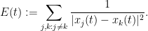
Again, there is the important technical issue that this quantity is infinite; but it turns out that if we renormalise the Hamiltonian appropriately, then the energy will also become suitably renormalised, and in particular will vanish when the are arranged in an arithmetic progression, and be positive otherwise. One can also formally calculate the derivative of to be a somewhat complicated but manifestly non-negative quantity (a sum of squares); see this previous blog post for analogous computations in the case of heat flow on polynomials. After flowing from time to time , and using some crude initial bounds on  and in this region (coming from the Riemann-von Mangoldt type formulae mentioned above and some further manipulations), we can eventually show that the (renormalisation of the) energy
  at time zero is small, which forces the to locally resemble an arithmetic progression, which gives the required convergence to local equilibrium.
There are a number of technicalities involved in making the above sketch of argument rigorous (for instance, justifying interchanges of derivatives and infinite sums turns out to be a little bit delicate). I will highlight here one particular technical point. One of the ways in which we make expressions such as the energy finite is to truncate the indices  to an interval
  to create a truncated energy
  . In typical situations, we would then expect to be decreasing, which will greatly help in bounding
  (in particular it would allow one to control by time-averaged quantities such as
  , which can in turn be controlled using variants of (4)). However, there are boundary effects at both ends of that could in principle add a large amount of energy into
  , which is bad news as it could conceivably make undesirably large even if integrated energies such as remain adequately controlled. As it turns out, such boundary effects are negligible as long as there is a large gap between adjacent zeroes at boundary of – it is only narrow gaps that can rapidly transmit energy across the boundary of . Now, narrow gaps can certainly exist (indeed, the GUE hypothesis predicts these happen a positive fraction of the time); but the pigeonhole principle (together with the Riemann-von Mangoldt formula) can allow us to pick the endpoints of the interval so that no narrow gaps appear at the boundary of for any given time . However, there was a technical problem: this argument did not allow one to find a single interval that avoided gaps for all times
  simultaneously – the pigeonhole principle could produce a different interval for each time ! Since the number of times was uncountable, this was a serious issue. (In physical terms, the problem was that there might be very fast “longitudinal waves” in the dynamics that, at each time, cause some gaps between zeroes to be highly compressed, but the specific gap that was narrow changed very rapidly with time. Such waves could, in principle, import a huge amount of energy into by time .) To resolve this, we borrowed a PDE trick of Bourgain’s, in which the pigeonhole principle was coupled with local conservation laws. More specifically, we use the phenomenon that very narrow gaps
  take a nontrivial amount of time to expand back to a reasonable size (this can be seen by comparing the evolution of this gap with solutions of the scalar ODE
  , which represents the fastest at which a gap such as
  can expand). Thus, if a gap is reasonably large at some time
  , it will also stay reasonably large at slightly earlier times
 ![{t \in [t_0-\delta, t_0]}](https://s0.wp.com/latex.php?latex=%7Bt+%5Cin+%5Bt_0-%5Cdelta%2C+t_0%5D%7D&bg=ffffff&fg=000000&s=0&c=20201002) for some moderately small
for some moderately small  . This lets one locate an interval that has manageable boundary effects during the times in
 ![{[t_0-\delta, t_0]}](https://s0.wp.com/latex.php?latex=%7B%5Bt_0-%5Cdelta%2C+t_0%5D%7D&bg=ffffff&fg=000000&s=0&c=20201002) , so in particular is basically non-increasing in this time interval. Unfortunately, this interval is a little bit too short to cover all of
, so in particular is basically non-increasing in this time interval. Unfortunately, this interval is a little bit too short to cover all of ![{[\Lambda/2,0]}](https://s0.wp.com/latex.php?latex=%7B%5B%5CLambda%2F2%2C0%5D%7D&bg=ffffff&fg=000000&s=0&c=20201002) ; however it turns out that one can iterate the above construction and find a nested sequence of intervals
; however it turns out that one can iterate the above construction and find a nested sequence of intervals  , with each
  non-increasing in a different time interval
 ![{[t_k - \delta, t_k]}](https://s0.wp.com/latex.php?latex=%7B%5Bt_k+-+%5Cdelta%2C+t_k%5D%7D&bg=ffffff&fg=000000&s=0&c=20201002) , and with all of the time intervals covering . This turns out to be enough (together with the obvious fact that is monotone in ) to still control for some reasonably sized interval , as required for the rest of the arguments.
, and with all of the time intervals covering . This turns out to be enough (together with the obvious fact that is monotone in ) to still control for some reasonably sized interval , as required for the rest of the arguments.
ADDED LATER: the following analogy (involving functions with just two zeroes, rather than an infinite number of zeroes) may help clarify the relation between this result and the Riemann hypothesis (and in particular why this result does not make the Riemann hypothesis any easier to prove, in fact it confirms the delicate nature of that hypothesis). Suppose one had a quadratic polynomial  of the form
  , where was an unknown real constant. Suppose that one was for some reason interested in the analogue of the “Riemann hypothesis” for , namely that all the zeroes of are real. A priori, there are three scenarios:
- (Riemann hypothesis false)
 , and has zeroes
  off the real axis.
- (Riemann hypothesis true, but barely so)
 , and both zeroes of are on the real axis; however, any slight perturbation of in the positive direction would move zeroes off the real axis.
- (Riemann hypothesis true, with room to spare) , and both zeroes of are on the real axis. Furthermore, any slight perturbation of will also have both zeroes on the real axis.
The analogue of our result in this case is that , thus ruling out the third of the three scenarios here. In this simple example in which only two zeroes are involved, one can think of the inequality as asserting that if the zeroes of are real, then they must be repeated. In our result (in which there are an infinity of zeroes, that become increasingly dense near infinity), and in view of the convergence to local equilibrium properties of (3), the analogous assertion is that if the zeroes of are real, then they do not behave locally as if they were in arithmetic progression.


71 comments
Comments feed for this article
19 January, 2018 at 4:26 am
Nikita Sidorov
Terry, I believe the link should be https://arxiv.org/abs/1801.05914
[Corrected, thanks – T.]
19 January, 2018 at 5:04 am
Anonymous
1. the link to the paper is wrong( https://arxiv.org/abs/1801.03908). It should probably be https://arxiv.org/pdf/1801.05914.pdf
2. Rodgers and I have uploaded to the arXiv _its_ paper
3. of Newman regarding _to_ the extent to which
4. Furthermore, this Hamiltonian _ _ a convex function
5. evolution of this gap _with_ with solutions
6. This lets one get _a_ locate an interval
[Corrected, thanks – T.]
19 January, 2018 at 6:30 am
Anonymous
“As observed by Csordas, Smith, and Vargas” it should be Varga without s
[Corrected, thanks – T.]
19 January, 2018 at 7:07 am
Anonymous
“have only real zeros” seems clearer than “have all real zeros”.
[Reworded – T.]
19 January, 2018 at 7:25 am
Anonymous
Since previous results used “Lehmer pairs”, is it possible that this result implies some new information on the behavior of “Lehmer pairs”?
19 January, 2018 at 7:45 am
Terence Tao
We don’t quite use the Csordas-Smith-Varga method to lower bound the de Bruijn-Newman constant using Lehmer pairs, because we were unable to produce a sufficiently strong sequence of such pairs without introducing powerful hypotheses such as GUE. (However, we were able to use the CSV method to give a shorter proof of our theorem conditional on the GUE hypothesis; this is not detailed in the preprint, but I might write this up in a separate blog post.) As such, we do not directly say anything new about these pairs.
One can compare the arguments in this way. CSV used the dynamics of zeroes (equation (3) in this blog post) to show that if the de Bruijn-Newman constant was significantly below zero, then any pair of adjacent zeroes of
  would be repelled from each other, in the sense that they could not be much closer to each other than to other nearby zeroes. Such repulsion would be in contradiction with the existence of sufficiently strong Lehmer pairs, which is why one can use a given Lehmer pair to produce a lower bound on
  . Our argument makes a more complicated analysis of the dynamics of (3) (incorporating the CSV arguments, but several other arguments besides, including ideas from Erdos-Schlein-Yau and Bourgain) to make a stronger assertion, namely that if the de Bruijn-Newman constant was significantly below zeroes, then the zeroes are not only repelled from each other, but are approximately in local equilibrium in the sense that they behave like an arithmetic progression at small scales. This type of behaviour was already ruled out from prior work on pair correlation (in particular by the work of Montgomery and Conrey-Ghosh-Gonek mentioned in the blog post).
So, basically to establish this result, we didn’t actually prove any new results about the distribution of zeroes of the zeta function, relying instead on existing literature. Instead, the main advance came from a better understanding of the dynamics of (3). (We also needed some coarse-scale control on the zeroes of which was not explicitly in prior literature, but which was obtainable from relatively standard, though lengthy, computations.)
19 January, 2018 at 9:44 am
New top story on Hacker News: The De Bruijn-Newman constant is non-negative – Tech + Hckr News
[…] The De Bruijn-Newman constant is non-negative 3 by lisper | 0 comments on Hacker News. […]
19 January, 2018 at 10:29 am
Aula
The second display above (1) is missing du at the end.
[Corrected, thanks – T.]
19 January, 2018 at 10:59 am
Anonymous
Assuming RH (i.e. by this result ), are these methods sufficient to improve on the current bound
  on the multiplicities of the zeros?
19 January, 2018 at 5:15 pm
Terence Tao
On RH I believe one can obtain a bound of on the multiplicity of zeroes (Theorem 14.13 of Titchmarsh). I am not aware of any further improvement. Our methods unfortunately don’t seem to say anything new about zeta in the actual world where
  ; they only give (unreasonably) strong control on zeta in the counterfactual world where
  .
.
19 January, 2018 at 11:12 am
The De Bruijn-Newman constant is non-negative - KISCAFE
[…] Read More […]
19 January, 2018 at 12:00 pm
Anonymous HN user
Posted on HN (HackerNews): https://news.ycombinator.com/item?id=16187499
19 January, 2018 at 1:50 pm
David Cole
Wow! Impressive effort! And Congratulations to you, Prof. Tao and Prof. Rodgers provided your work, proof of Newman’s Conjecture, is rings true!
On the Riemann Hypothesis, your ‘barely’ is not the best way to state perfection or Λ =0 (assuming your proof is correct) via the Newman’s Conjecture with regards to the truth of the Riemann Hypothesis.
FYI:
https://www.researchgate.net/post/Does_the_nth_nontrivial_simple_zero_of_the_Riemann_Zeta_Function_indicate_the_nth_prime_p_n_occurs_as_a_prime_factor_in_all_multiples_of_p_n
19 January, 2018 at 1:59 pm
David Cole
Oops!
“… rings true!” Your proof assuming it rings true is still a long away from affirming the truth of the Riemann Hypothesis.
But, please trust me (or my work on the Riemann Hypothesis).
The Riemann Hypothesis is true! :-)
19 January, 2018 at 4:21 pm
De Bruijn-Newman meets Riemann – The nth Root
[…] …. (Terence Tao) […]
19 January, 2018 at 10:32 pm
Anonymous
So Λ should be 0 ?
20 January, 2018 at 1:19 am
Anonymous
In the preprint, for equation 38 and 39, there is a constant difference of -\frac{\ln4\pi}{4\pi} between the derivative of 38 and what is written for 39. Does this have anything to do with equation 37 being an asymptotic relationship?
20 January, 2018 at 3:31 am
Terence Tao
Yes, one can absorb this constant factor into the error.
20 January, 2018 at 2:59 am
Anonymous
Is the currently known best explicit(!) upper bound on still
still  ?
?
20 January, 2018 at 3:34 am
Terence Tao
Yes, although Ki, Kim, and Lee have improved the bound a tiny bit from to
to  . It may be possible to do better than this by refining the Riemann-von Mangoldt formulae for H_t in our paper, as well as somehow numerically verifying the Riemann hypothesis for
  up to some large height (possibly leveraging the existing numerical verification for the zeta function), but I have not tried to do this in detail.
20 January, 2018 at 4:19 am
Anonymous
Is there any known 1:1 correspondence between (the possible value of)
 and (the possible value of) the supremum (
 ,say) on the real parts of zeta zeros ?
 implies that
  as well !
If so, it seems that the result
20 January, 2018 at 6:19 am
Terence Tao
I think there is a relation of the form (this follows for instance from Theorem A of the Ki-Kim-Lee paper after a little bit of effort). Roughly speaking, this relation arises from the attraction that a zero off the critical line will feel from its reflected partner on the other side of the line when evolving under backwards heat flow. However this is not the only source of attraction – the other zeroes will also pull at this zero – so I doubt that one can hope to reverse this inequality exactly (other than by proving
  and
and  , of course). Indeed the Ki-Kim-Lee paper is in some sense showing that this sort of relationship between
  and
and  is not optimal, and does not give any new results on
  .
.
20 January, 2018 at 7:41 am
Anonymous
My question was motivated by observing that the parameter plays the role of a “regulating parameter” in the sense that if
  has only real zeros, then so is
  for any
  .
. has a kind of “regulating effect” on the zeros of
  in the sense of keeping them on the real axis.
 for which
  has all its zeroes in a strip
  for some positive
  which is the supremum over the imaginary parts of the zeros of
  . A natural generalization of the regulating effect for such
  is that by increasing
  , the zeros of
  tend to decrease their distances from the real axis (i.e. are “attracted” by the real axis), and in particular, the function
  should (strictly?) decrease with increasing
  . Hence, the constant
  may be viewed as the minimal value of the parameter
  needed to “pull back” the zeros of
  (assuming
  ) into the real axis (i.e.
  ). Since
  is closely related with
  , the extended regulating effect seems to imply that
  should (strictly?) increase with increasing
  .
.
So increasing
Hence a natural question is whether this regulating effect may have an extension to include also the case of parameters
20 January, 2018 at 10:56 am
Terence Tao
One has the differential inequality
whenever , basically because of the attraction between any zero
  off the real axis to its conjugate
  . (Again, see the Ki-Kim-Lee paper for more details.) Combining this with
  gives the bound
  I mentioned in my previous comment. However, this inequality will not be an equality in general, due to the additional attraction that such a zero will also experience with respect to the remaining zeroes of
  . This latter effect is complicated and does not necessarily behave in a monotone fashion with respect to
  or
or  (actually, it’s hard to quantify exactly what such a monotonicity would even mean, given that
  is an absolute constant rather than a parameter). So it could be that a configuration of zeroes with a larger value of
  could in fact have a faster convergence to the real axis than a different configuration with a smaller value of
  due to these other effects. As such, I doubt that there is any particularly clean relationship between
  and
and  , though one could still hope to improve upon the Ki-Kim-Lee analysis.
20 January, 2018 at 7:34 pm
Anonymous
It seems that in order to use this approach to show that , one needs also a good lower bound for the derivative
  (sufficiently close to the upper bound above) to get a sufficiently good estimate on the dependence of
  on
on  such that a sufficiently good explicit(!) upper bound on
  (e.g. by refining the Ki-Kim-Lee merhod) would give an explicit new upper bound on
  .
.
21 January, 2018 at 12:31 pm
Anonymous
It is interesting to observe that since for there are only finitely many non-real zeros of
  (by theorem 1.3 of the KKL paper), the function
  (defined as the supremum over the imaginary parts of
  zeros) is actually attained by the imaginary part of some non-real zero of
  whenever
  – showing that
  is determined by the dynamics of that zero – so it is not only (piecewise) differentiable but even piecewise analytic (it may not be analytic for those
  values for which it is attained by the imaginary parts of at least two non-real zeros of
  ).
).
20 January, 2018 at 10:42 am
Anonymous
If a large scale computational effort can help in upper bounding the constant, I think several people would want to help. Do write more on this.
21 January, 2018 at 3:55 am
Terence Tao
In principle one could do this as follows. The analysis of Ki-Kim-Lee (see in particular the proof of Proposition 3.1 of their paper) shows that for any and
and  , there exists
  such that there are no zeroes
  with
with  and
and  . They do not explicitly compute
  in terms of
  and
and  , but it could in principle be made effective. If it is not too large, one could also numerically verify (e.g. by argument principle and quadrature) that all zeroes of
  with real part in
 ![[0,T]](https://s0.wp.com/latex.php?latex=%5B0%2CT%5D&bg=ffffff&fg=545454&s=0&c=20201002) have imaginary part less than
have imaginary part less than  . Combining this with Proposition A of Ki-Kim-Lee gives an upper bound of the form
  , so presumably for
  small enough one can improve upon the bound of
  (of course, making
  smaller will make
  larger).
One could possibly envisage a Polymath style project in this direction, which would naturally split into two halves: a computational effort to establish rectangular zero-free regions for
for  , and an optimisation of the KKL arguments to obtain an explicit dependence of
  on
on  . [EDIT: there is also a third direction, which is to try to improve the bound
  by using the dynamics of zeroes.] If there is enough interest I would be willing to launch and moderate such a project.
21 January, 2018 at 6:32 am
Anonymous
I strongly support such Polymath style project! , say) the argument of the integrand on a sufficiently dense set of “grid points” on the rectangular integration contour such that the argument increment between any two consecutive grid points is assured(!) to remain sufficiently small (e.g. less than
  in absolute value).
 there are at most finitely many non-real zeros of
  – so even for
  , there is a finite corresponding
  (but its numerical estimation seems to be much more difficult).
 , the zeros of
  are distributed much more regularly with better asymptotic estimates than the zeros of
  – which might help in estimating their dynamics (in the third direction of the suggested project).
Some remarks:
1. In practice, to use the argument principle one needs only to compute approximately (with precision better than
2. By theorem 1.3 of the KKL paper, for each
3. By theorem 1.4 of the KKL paper, for each
21 January, 2018 at 10:44 am
Anonymous
I too support the idea of a Polymath project for this. As the other reply said, Theorem 1.3 of KKL finally mentions only T and not epsilon which makes this quite exciting but presumably much more difficult.
It would also be quite interesting to see the magnitude of T for extremely small positive t values once the explicit dependence is established, even if the computational effort for such t gets prohibitive.
23 January, 2018 at 6:41 am
Brad
I also would be interested such a polymath. If we make progress on the size of for
for  , it may also be interesting to consider somewhat more general questions: e.g. for an entire function
  with rapidly decaying real and even Fourier transform, and with a Riemann – von Mangoldt formula akin to that for
  (that is, with the same asymptotic form and error term, and which counts zeros in the same critical strip), how large can
  for the function
  be? De Bruijn gives in general
  , but it’s not clear to me if this is optimal when zeros increase in density along the critical strip. (This may already be in the literature, but I’m not aware of a reference.)
23 January, 2018 at 7:18 am
nicodean
i would love to participate at some point to such a project. while i am no number theoretist, i could maybe help on the numerics (at least i would really like to follow the numerics-part of the project closely to understand these approaches better).
20 January, 2018 at 10:58 am
Lehmer pairs and GUE | What's new
[…] is non-negative. This implication is now redundant in view of the unconditional results of this recent paper of myself and Rodgers; however, the question of whether an infinite number of Lehmer pairs exist remain […]
20 January, 2018 at 12:55 pm
jm
Is there an analogue of your result for the function-field RH, and does it become something easier there?
20 January, 2018 at 7:17 pm
Terence Tao
This was investigated by Chang et al., see https://www.math.cornell.edu/~dmehrle/research/papers/newmanpaper-final.pdf
20 January, 2018 at 8:19 pm
Ahmad Heydari
thank’s for share this article
22 January, 2018 at 12:41 pm
Michel Eve
I have a basic and perhaps naïve question about the Newman conjecture now a theorem. Generally a conjecture is an assumption which allows further important results (like RH in prime number theory) or can be readily understood by non mathematicians (like FLT which was not a theorem until 1994).I understand from reading your comments that this new theorem does not help much to solve RH and it is far too complex to mean anything to the general public. So what is its usefulness ? One could be tempted to try to lower the constant upper bound down to zero but is this avenue more promising than other approaches to solve RH ? Can it be used to make progress in other areas of number theory ?
22 January, 2018 at 2:02 pm
Terence Tao
Besides the possibility of immediate applications (which are indeed somewhat slim), or the historical interest of settling a question that had attracted a fair amount of previous literature, I think this result will help demystify somewhat the functions introduced by de Bruijn, and in particular emphasise the role of both ODE and oscillatory integral estimates in understanding them further. If in the future it turns out that these functions – or other functions similar to them – have additional interesting properties to exploit (e.g. some variant of an Euler product factorisation), then one could well have some unexpected application of the existing literature on these functions, including my paper with Brad. But I think it is also justifiable to study these questions for their own sake.
24 January, 2018 at 7:57 am
Gil Kalai
Congratulations Brad and Terry. Two very naive question.One is if the Cramer probabilistic heuristic gives reason to think that Lambda is 0. (or some other simple heuristic reason.) The second is if the the heat flow of the zeta is the same or analogous to a zeta function of some “perturbation” of the primes. (beurling primes) E.g. you create a new sequence of “primes” with precisely the same density where you take p_n 0,1,2… times according to some probability distribution (perhaps depending on n) with expectation one.
24 January, 2018 at 9:05 am
Terence Tao
Actually that seems to be the one key thing that the de Bruijn perturbations of
of  (which is essentially the Riemann xi function) is lacking – they do have analytic continuation and a functional equation, but they are missing anything resembling an Euler product that would relate them to something resembling prime numbers. So, at least at our current level of understanding, they are largely objects of an analytic nature rather than an arithmetic one. It in fact seems remarkably hard to deform the Riemann zeta function in a way that keeps both the functional equation structure and the Euler product structure; the known examples of such functions (basically the Selberg class) are very arithmetic in nature, with no continuous parameter to deform in.
24 January, 2018 at 9:40 am
Gil Kalai
I see, out of curiosity: you can consider Beurling primes where is taken with probability
  , where
  goes to zero as quickly as you wish. This will lead to some deformation of the zeta function. Do all the desirable properties zeta and the statistical properties of primes disappear no matter how quickly these delta’s tends to 0?
24 January, 2018 at 4:02 pm
Terence Tao
I think the functional equation is all but guaranteed to be destroyed when modifying the zeta function in this fashion. The functional equation is basically reflecting the fact that the multiplicative semigroup generated by the primes – that is to say, the natural numbers – is essentially an abelian group with respect to addition (it is one half of the integers), and so enjoys a Poisson summation formula which eventually becomes the functional equation. If one randomly perturbs the set of primes, there is no longer any reason to expect additive structure in the semigroup generated by the remaining primes.
To put it another way, the Euler product reflects the multiplicative structure of the integers, whereas the functional equation reflects the additive structure. It’s hard to perturb the integers to retain both structures (other than to work with other rings of algebraic integers or similar objects, of course).
24 January, 2018 at 6:53 pm
Anonymous
Perhaps there is a way to formulate a necessary and sufficient condition for such a continuous (preferably differentiable) perturbation probably in terms of some differential equation?
25 January, 2018 at 12:10 am
Gil Kalai
Putting Beurling primes aside. Had been negative, were there some implications on the distribution of primes stronger than those given by RH. Similarly if one proves say
  , would it have any implications on the distribution of primes (weaker, of course, than those given by RH)?
25 January, 2018 at 8:10 am
Terence Tao
The literature so far has almost exclusively focused on implications of the form “information about zeroes of zeta” -> “information about the de Bruijn-Newman constant”, with the notable exception of course of the implication . It is conceivable that one could work on the converse and eventually show, for instance, that smallness of
  implies a zero free region for zeta which in turn implies some reasonably good error term in the prime number theorem. But given that our project to bound
  will use, among other things, numerical zero free regions for zeta and related functions, I would imagine that this would be an extremely inefficient route to get new information about zeta.
24 January, 2018 at 3:54 pm
Polymath proposal: upper bounding the de Bruijn-Newman constant | What's new
[…] on the interest expressed in the comments to this previous post, I am now formally proposing to initiate a “Polymath project” on the topic of obtaining […]
25 January, 2018 at 5:13 am
El duro camino hacia la demostración de la hipótesis de Riemann | Ciencia | La Ciencia de la Mula Francis
[…] matemáticos) en Terence Tao, “The De Bruijn-Newman constant is non-negative,” What’s new, 19 Jan 2018. Sabemos que 0 ≤ Λ < 1/2, reducir esta cota superior es el objetivo del nuevo proyecto […]
25 January, 2018 at 11:17 pm
A new polymath proposal (related to the Riemann Hypothesis) over Tao’s blog | The polymath blog
[…] Terry Tao’s blog who wrote: “Building on the interest expressed in the comments to this previous post, I am now formally proposing to initiate a “Polymath project” on the topic of obtaining new […]
27 January, 2018 at 4:10 pm
Polymath15, first thread: computing $H_t$, asymptotics, and dynamics of zeroes | What's new
[…] real part on this strip. One can use the Poisson summation formula to verify that is even, (see this previous post for details). This lets us obtain a number of other formulae for . Most obviously, one can unfold […]
28 January, 2018 at 8:58 pm
Anonymous
THE DE BRUIJN NEWMAN CONSTANT IS POSITIVE IF THE “FAMOUS” RIEMANN HYPOTHESIS IS WRONG. AS THE TITLE OF THIS BLOG POST SUGGESTS, COULD THIS BE A STEP TO DISPROVING THE RIEMANN HYPOTHESIS?
2 February, 2018 at 8:55 pm
Polymath15, second thread: generalising the Riemann-Siegel approximate functional equation | What's new
[…] real part on this strip. One can use the Poisson summation formula to verify that is even, (see this previous post for details). This lets us obtain a number of other formulae for . Most obviously, one can unfold […]
7 June, 2018 at 3:15 am
Heat flow and zeroes of polynomials II: zeroes on a circle | What's new
[…] arguments in my paper with Brad Rodgers (discussed in this previous post) indicate that for a “typical” polynomial of degree that obeys the Riemann […]
14 August, 2018 at 9:06 pm
Irfan Ali
That’s a great move towards a Problem of Riemann I am student of MS Applied mathematics at IBA Sukkur University Sindh,Pakistan also working on the Problem but still iam reading the work which has done towards Riemann Hypothesis what would be the next move ?
working on constant is zero and see what happens either contradiction happens or not?
Or working in the region (0,0.22)?
Now which difficulties arises to work on the Newman constant is 0 or greater than 0?
10 October, 2018 at 9:55 am
Watching Over the Zeroes | Gödel's Lost Letter and P=NP
[…] to a possible argument that the RH is false. In January of this year, Brad Rogers and Terence Tao turned up the heat on this connection by proving that the GUE conjecture entails the existence of […]
28 February, 2019 at 5:30 am
Dan Romik Studies the Riemann’s Zeta Function, and Other Zeta News. | Combinatorics and more
[…] It is now the 10 year anniversary of polymath projects and let me belatedly mention a successful project polymath15 that took place over Terry Tao blog. The problem is related to the Hermite expansion of the Zeta function. Roughly speaking you can apply a noise operator on Zeta that causes higher degrees to decay exponentially. (The noise can be “negative” and then the higher degrees explode exponentially.) The higher the amount t of noise the easier the assertion of the Riemann Hypothesis (RH) becomes. Let , the de Bruijn-Newman constant, be the smallest amount of noise under which the assertion of RH is correct. It was conjectured that namely the assertion of the RH fails when you apply negative noise no matter how small. This follows from known conjectures on the spacing between zeroes of the Zeta function since when the assertion of RH is known for some level (positive or negative) of noise, then with a higher level of noise spacing between zeroes become more boring. The conjecture was settled by Brad Rodgers and Terry Tao. (See this blog post by Terry Tao.) […]
9 July, 2019 at 3:55 am
Isaac TK
Dear Prof. Tao, in your video lecture, ”Vaporizing and freezing the Riemann zeta function,” Prof. Tao, in your video lecture, ”Vaporizing and freezing the Riemann zeta function https://www.youtube.com/watch?v=t908N5gUZA0,” you said
”De Bruijn showed that if for some real the zeros of
  are contained in the horizontal strip
  , then \textit{for all}
  , they will be contained in a narrower strip
where are real. Note that
  , where
  denotes the Riemann xi function. Since
  for
for  , we can take
  ,
,  ,
,  where
where  is an arbitrarily small positive number, and deduce that all the zeros of
  must be real for
  . This implies that if all zeros of
  are real if and only if
  , then
  , (the Riemann Hypothesis !)
This would mean that de Bruijn proved the RH, but did not realize it !
10 July, 2019 at 10:54 am
Terence Tao
This argument gives real zeroes of only for
  , not for all
  .
.
2 September, 2019 at 1:06 am
Anonymous1
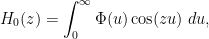
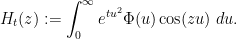
Dear Prof Tao, recall that for one has
  . By the mean-value theorem for integrals, it follows that
  for some real number
  . By your intuition, $H_t$ can be regarded as a ´piece of matter´ and exists in gaseous form for
  . So doesn the above equation entail that $H_0$ must also be a gas ?
2 September, 2019 at 5:46 am
Terence Tao
The mean value theorem is only valid for real-valued functions, not complex-valued ones. For instance, is the mean of
  , but
, but  for any
  .
.
2 September, 2019 at 6:14 am
Anonymous1
Oh sure, had overlooked that, so must be real, which leads me to the following question: doesn’t the equation
  for some real number
  and
and  entail that
  should have an Euler product since
  has one ?
2 September, 2019 at 6:18 am
Anonymous1
Recall that is real whenever
  is real.
2 September, 2019 at 6:22 am
Anonymous1
Typo at the end of my previous comment: there should be a instead of a
  .
.
2 September, 2019 at 6:54 am
Anonymous1
In particular, since the RH is equivalent to the statement that all local minima of are negative and all of its local maxima are positive, the equality
  yields a reformulation of the RH in terms of
  ! See my question on MathOverflow https://mathoverflow.net/q/339698/145279. Since the function $H_t$ has proved to be much easier to deal with, a Polymath paper can come out of the above reformulation. However, if it is already known that all local minima of
  are negative and all local maxima are negative, then the RH follows. If the opposite is known, then the RH is false.
2 September, 2019 at 6:56 am
Anonymous1
See also my MathOverflow question https://mathoverflow.net/q/339698/145279
13 May, 2020 at 7:27 am
Terence Tao
Making a short note here that my student Alexander Dobner has found a simpler proof of Newman’s conjecture that uses complex analysis instead of PDE type arguments, and extends from the zeta function to quite general Dirichlet series: https://arxiv.org/abs/2005.05142
13 May, 2020 at 2:20 pm
Anonymous
Is it possible to find non-trivial upper bounds also for the corresponding de Bruijn-Newman constants of more general Dirichlet series?
14 May, 2020 at 6:59 am
Terence Tao
Nice question! The original work of Polya already gives an upper bound for the dBN constant of any Dirichlet series obeying a functional equation in terms of the width of a strip known to contain all the zeroes of the (completed) series. It may well be possible to adapt the work of Ki, Kim, and Lee to improve this bound slightly from a non-strict inequality to a strict inequality. The methods of the new paper of Dobner will probably not be of direct use though, it is based on approximations to the modified function (related to the function
  in the notation of my paper with Rodgers) that are accurate for
  , which is the regime one would need to study for the upper bound problem.
26 August, 2021 at 12:47 pm
aaa108
Does this result fall under any positivity paradigm?
26 August, 2021 at 12:48 pm
aaa108
By this I mean can you translate this result to the purported approaches through modifying Deligne’s works? If not why and if yes how to think about it?
23 December, 2022 at 6:55 pm
Anonymous
Thanks T.
22 January, 2023 at 12:43 am
TK
If you’re well-versed in basic complex analysis and basic analytic number theory, i kindly invite you to judge this 4-page paper for yourself:
https://figshare.com/articles/preprint/Untitled_Item/14776146