This is a sequel to this previous blog post, in which we discussed the effect of the heat flow evolution
on the zeroes of a time-dependent family of polynomials  , with a particular focus on the case when the polynomials had real zeroes. Here (inspired by some discussions I had during a recent conference on the Riemann hypothesis in Bristol) we record the analogous theory in which the polynomials instead have zeroes on a circle
  , with the heat flow slightly adjusted to compensate for this. As we shall discuss shortly, a key example of this situation arises when
  is the numerator of the zeta function of a curve.
More precisely, let  be a natural number. We will say that a polynomial
of degree  (so that
  ) obeys the functional equation if the
  are all real and
for all  , thus

and
for all non-zero  . This means that the zeroes
  of
of  (counting multiplicity) lie in
  and are symmetric with respect to complex conjugation
  and inversion
  across the circle
  . We say that this polynomial obeys the Riemann hypothesis if all of its zeroes actually lie on the circle
  . For instance, in the
  case, the polynomial
  obeys the Riemann hypothesis if and only if
  .
.
Such polynomials arise in number theory as follows: if  is a projective curve of genus over a finite field
  , then, as famously proven by Weil, the associated local zeta function
  (as defined for instance in this previous blog post) is known to take the form

where is a degree polynomial obeying both the functional equation and the Riemann hypothesis. In the case that is an elliptic curve, then and takes the form  , where
  is the number of
  -points of minus
  . The Riemann hypothesis in this case is a famous result of Hasse.
Another key example of such polynomials arise from rescaled characteristic polynomials

of  matrices
  in the compact symplectic group
  . These polynomials obey both the functional equation and the Riemann hypothesis. The Sato-Tate conjecture (in higher genus) asserts, roughly speaking, that “typical” polyomials arising from the number theoretic situation above are distributed like the rescaled characteristic polynomials (1), where is drawn uniformly from with Haar measure.
Given a polynomial  of degree with coefficients

we can evolve it in time by the formula
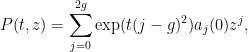
thus  for
for  . Informally, as one increases
  , this evolution accentuates the effect of the extreme monomials, particularly,
  and
and  at the expense of the intermediate monomials such as
  , and conversely as one decreases . This family of polynomials obeys the heat-type equation

In view of the results of Marcus, Spielman, and Srivastava, it is also very likely that one can interpret this flow in terms of expected characteristic polynomials involving conjugation over the compact symplectic group  , and should also be tied to some sort of “
 ” version of Brownian motion on this group, but we have not attempted to work this connection out in detail.
It is clear that if obeys the functional equation, then so does for any other time . Now we investigate the evolution of the zeroes. Suppose at some time  that the zeroes
  of
of  are distinct, then

From the inverse function theorem we see that for times sufficiently close to , the zeroes  of continue to be distinct (and vary smoothly in ), with
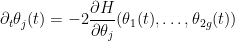
Differentiating this at any not equal to any of the  , we obtain

and

and

Inserting these formulae into (2) (expanding  as
as  ) and canceling some terms, we conclude that


for sufficiently close to , and not equal to . Extracting the residue at  , we conclude that

which we can rearrange as

If we make the change of variables  (noting that one can make
  depend smoothly on for sufficiently close to ), this becomes

Intuitively, this equation asserts that the phases repel each other if they are real (and attract each other if their difference is imaginary). If obeys the Riemann hypothesis, then the are all real at time , then the Picard uniqueness theorem (applied to  and its complex conjugate) then shows that the are also real for sufficiently close to . If we then define the entropy functional

then the above equation becomes a gradient flow
which implies in particular that  is non-increasing in time. This shows that as one evolves time forward from , there is a uniform lower bound on the separation between the phases
  , and hence the equation can be solved indefinitely; in particular, obeys the Riemann hypothesis for all
  if it does so at time . Our argument here assumed that the zeroes of were simple, but this assumption can be removed by the usual limiting argument.
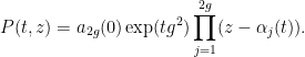
For any polynomial obeying the functional equation, the rescaled polynomials  converge locally uniformly to
  as
as  . By Rouche’s theorem, we conclude that the zeroes of converge to the equally spaced points
  on the circle . Together with the symmetry properties of the zeroes, this implies in particular that obeys the Riemann hypothesis for all sufficiently large positive . In the opposite direction, when
  , the polynomials converge locally uniformly to
  , so if
  , of the zeroes converge to the origin and the other converge to infinity. In particular, fails the Riemann hypothesis for sufficiently large negative . Thus (if ), there must exist a real number
  , which we call the de Bruijn-Newman constant of the original polynomial , such that obeys the Riemann hypothesis for
  and fails the Riemann hypothesis for
  . The situation is a bit more complicated if
  vanishes; if
  is the first natural number such that
  (or equivalently,
  ) does not vanish, then by the above arguments one finds in the limit that
  of the zeroes go to the origin, go to infinity, and the remaining
  zeroes converge to the equally spaced points
  . In this case the de Bruijn-Newman constant remains finite except in the degenerate case
  , in which case
  .
.
For instance, consider the case when and  for some real with . Then the quadratic polynomial
has zeroes

and one easily checks that these zeroes lie on the circle  when
when  , and are on the real axis otherwise. Thus in this case we have
  (with
(with  if
if  ). Note how as increases to
  , the zeroes repel each other and eventually converge to
  , while as decreases to
  , the zeroes collide and then separate on the real axis, with one zero going to the origin and the other to infinity.
The arguments in my paper with Brad Rodgers (discussed in this previous post) indicate that for a “typical” polynomial of degree that obeys the Riemann hypothesis, the expected time to relaxation to equilibrium (in which the zeroes are equally spaced) should be comparable to  , basically because the average spacing is and hence by (3) the typical velocity of the zeroes should be comparable to , and the diameter of the unit circle is comparable to
  , thus requiring time comparable to to reach equilibrium. Taking contrapositives, this suggests that the de Bruijn-Newman constant should typically take on values comparable to
  (since typically one would not expect the initial configuration of zeroes to be close to evenly spaced). I have not attempted to formalise or prove this claim, but presumably one could do some numerics (perhaps using some of the examples of given previously) to explore this further.


18 comments
Comments feed for this article
7 June, 2018 at 6:10 am
Anonymous
It seems that Riemann zeta function (whose zeros are pseudo-randomly distributed) can’t be interpreted (in any sense) as some “limiting case” of the above local zeta functions (having uniformly distributed zeros.)
8 June, 2018 at 1:56 pm
Joseph
I would have the intuition that maybe the value of should be closer to zero than
  because of the zeros which are close to each other: if the closest pair of zeros has distance
  and if we run the flow backwards, then they attract each other with speed about
  , and then would collide at time about
  if we neglect the other zeros (which are at much larger distance). For characteristic polynomial of
  where
where  has order
  , I would expect
  of about
  if my intuition is correct.
9 June, 2018 at 6:54 am
Terence Tao
Hmm, I think you’re right; the time to relaxation to equilibrium gives a lower bound on but it is far from optimal.
In the case of zeroes on the real line, there is a criterion of Csordas, Smith and Varga (see Theorem 1 of https://link.springer.com/article/10.1007/BF01205170 ) that says, roughly speaking, that if one has a pair of zeroes at separation , and the other zeroes are significantly further away from this pair than
  , then
  . It may well be that an analogous result holds on the circle.
9 June, 2018 at 1:01 pm
Joseph
I think it is equivalent to have points on the circle or all the determinations of their arguments on the real line (which gives a -periodic set), because of the formula
  .
.
9 June, 2018 at 8:35 am
Aula
The third display above (3) is too wide.
[Corrected, thanks – T.]
9 June, 2018 at 10:04 am
Will Sawin
It should possible to obtain the “time to relaxation” upper bound using only the middle coefficient. It has variance , so it is presumably typically of size
  , meaning at time
  , it is of size
  compared to the first and last coefficients, compared to the bound
  for polynomials with all roots on the unit circle.
18 June, 2018 at 9:22 am
Anonymous
Dear Terry,
I am not an expert mathematician.But I think the Riemann’s difficult level is 5 times more than Poincare.Because one only needs one way to go to the destination,Riemann must has 5 ways done:straight and then go back,attack the middle point,the first point and then the final point.And not enough, you must go with the first step on the old road many times.I know Terry very well.Someday not so long,the community of maths has amusing news from Terry.
Best wishes,
(Company of Pro.Tao -two decades)
2 July, 2018 at 3:16 pm
curious
Does the entropy here have anything do with information?
16 August, 2018 at 9:19 am
Tatenda Kubalalika
Dear Prof. Tao, according to equation of your paper with Prof. Rodgers, “the de Bruijn-newman constant is nonnegative”, the de Bruijn-Newman constant seems to be equal to
  .
.
Indeed, for , we have
Notice that the right-hand side is invariant under the transformation , thus we have
for all . Suppose that
  for some real
  hence
hence  . But we know by a result of Rodgers and Tao that
  for any
  and
and  . Thus we arrive at a contradiction,, which entails that our supposition must be false, and the desired result follows.
16 August, 2018 at 2:30 pm
Terence Tao
Unfortunately, the identity (1) is only valid for (as you point out), hence the identity (2) is only valid when
  , that is to say it is only established in the case
  (where it is trivial). Actually, one can check numerically that (2) is false in general.
16 August, 2018 at 11:59 pm
Anonymous
Since in (1) (for )
)  can be replaced by
  , is it possible that this modification of (1) (with the resulting branch point at
  due to
  ) still holds for some analytic continuation (with respect to
  ) of the modified integral ?
17 August, 2018 at 6:23 pm
Terence Tao
For positive t, one has
(see the equation before (35) in https://github.com/km-git-acc/dbn_upper_bound/blob/master/Writeup/debruijn.pdf ).
16 August, 2018 at 2:50 pm
Tatenda Kubalalika
Thank you for your response. Do you have any specific $t$ (or t’s) in mind for which (2) is false ? Because it seems to me that $H_{t}(z)$ is the Fourier transform of $\phi(t)e^{zt^2}$, which is an even function. This seems to imply that $H_t$ should also be even. That is, $H_{t}(z)=H_{-t}(z)$ for all real $t$. Of course, my reasoning could be flawed.
16 August, 2018 at 4:28 pm
TK
My mistake indeed in the last comment: i made a typo in the above Fourier transform, which invalidates the argument.
24 August, 2018 at 2:45 am
Tate. I. K
Indeed, the de Bruijn-Newman constant could be equal to zero.
Suppose there exists some pair of real numbers with
  , such that
 . It is a classical fact that
  as many real zeros, and let
  be one such zero, where
  is some real number. That is,
  We shall refer to this as equation
  . Combining equations
  and
and  yields
 We shall refer to this as equation
  As noted in Rodgers and Tao’s paper (page 3), one can view
  as the evolution of
  under the backwards heat equation
  , where
  denotes the time. Hence from equation
  we deduce that,“one can view
  as the EVOLUTION of
  ” But this quoted statement is meaningless, since both
  and
and  represent the same time
  .
.
$\latex H_{T}(z)=0.$ We shall refer to this as equation
We therefore conclude that our supposition must be false, and the desired result follows. $\square$ equal to zero.
24 August, 2018 at 2:20 pm
Terence Tao
(a) There certainly do exist pairs of real numbers with
  and
and  . In fact, it is a result of Ki, Kim and Lee that for
  , there are infinitely many zeroes of
  , all but finitely many of which are real.
(b) You have only shown that the equation holds for a single value of
  , not for all
  . The evolution of the heat equation does not depend only on the pointwise value of the initial data at a single value of
  , but on the values at all other positions as well (the heat equation has infinite speed of propagation).
24 August, 2018 at 2:57 am
Anonymous commenter.
@Tate. I. K, it really seems that you have demonstrated that . However, your argument is suspiciously short. It will be truly strange if such a long-standing problem as the RH could have such a short solution. I suggest that you submit your work to a formal journal, and goodluck !
28 April, 2022 at 12:43 pm
Brian C. Hall
In Section 2.3 of a recent preprint of mine with Ching-Wei Ho, we studied (essentially) this evolution from a random matrix point of view. Suppose, for example, that you start with the characteristic polynomial of a Brownian motion in the unitary group and then evolve toward negative time. We conjecture that the roots will rapidly move off the unit circle and that they will eventually resemble the eigenvalues of a Brownian motion in the general linear group. See https://arxiv.org/abs/2202.09660