
We now turn to the local existence theory for the initial value problem for the incompressible Euler equations


For sake of discussion we will just work in the non-periodic domain 


Formally, the Euler equations (with normalised pressure) arise as the vanishing viscosity limit 

that was studied in previous notes. However, because most of the bounds established in previous notes, either on the lifespan 


Nevertheless, by carefully using the energy method (which we will do loosely following an approach of Bertozzi and Majda), it is still possible to obtain local-in-time estimates on (high-regularity) solutions to (3) that are uniform in the limit

becomes infinite at the final time 
There is a rather different approach to establishing local well-posedness for the Euler equations, which relies on the vorticity-stream formulation of these equations. This will be discused in a later set of notes.
— 1. A priori bounds —
We now develop some a priori bounds for very smooth solutions to Navier-Stokes that are uniform in the viscosity 


Here are our first bounds:
Theorem 1 (A priori bound) Let
- (i) For any integer
, we have
Furthermore, if
for a sufficiently small constant
depending only on
, then
- (ii) For any
and integer
, one has


![\displaystyle \| u \|_{L^\infty_t H^s_x([0,T] \times{\bf R}^d \rightarrow {\bf R}^d)} \lesssim_{s,d}](https://s0.wp.com/latex.php?latex=%5Cdisplaystyle++%5C%7C+u+%5C%7C_%7BL%5E%5Cinfty_t+H%5Es_x%28%5B0%2CT%5D+%5Ctimes%7B%5Cbf+R%7D%5Ed+%5Crightarrow+%7B%5Cbf+R%7D%5Ed%29%7D+%5Clesssim_%7Bs%2Cd%7D+&bg=ffffff&fg=000000&s=0&c=20201002)
![\displaystyle \exp( O_{s,d}( \| \nabla u \|_{L^1_t L^\infty_x([0,T] \times {\bf R}^d \rightarrow {\bf R}^{d^2})} ) ) \| u_0 \|_{H^s_x({\bf R}^d \rightarrow {\bf R}^d)}.](https://s0.wp.com/latex.php?latex=%5Cdisplaystyle+%5Cexp%28+O_%7Bs%2Cd%7D%28+%5C%7C+%5Cnabla+u+%5C%7C_%7BL%5E1_t+L%5E%5Cinfty_x%28%5B0%2CT%5D+%5Ctimes+%7B%5Cbf+R%7D%5Ed+%5Crightarrow+%7B%5Cbf+R%7D%5E%7Bd%5E2%7D%29%7D+%29+%29+%5C%7C+u_0+%5C%7C_%7BH%5Es_x%28%7B%5Cbf+R%7D%5Ed+%5Crightarrow+%7B%5Cbf+R%7D%5Ed%29%7D.&bg=ffffff&fg=000000&s=0&c=20201002)
The hypothesis that
We now prove this theorem using the energy method. Using the Navier-Stokes equations, we see that 

![{L^\infty_t H^\infty_x([0,T] \times {\bf R}^d \rightarrow {\bf R}^d)}](https://s0.wp.com/latex.php?latex=%7BL%5E%5Cinfty_t+H%5E%5Cinfty_x%28%5B0%2CT%5D+%5Ctimes+%7B%5Cbf+R%7D%5Ed+%5Crightarrow+%7B%5Cbf+R%7D%5Ed%29%7D&bg=ffffff&fg=000000&s=0&c=20201002)

Let 
Here we think of 


where we suppress explicit dependence on 
where


For 


so in particular 

Now we expand out 


But we can locate a total derivative to write this as

and then an integration by parts using 

At this point we now need a variant of Proposition 35 from Notes 1:
Exercise 2 Let
be integers. For any
, show that
(Hint: for
or
, use Hölder’s inequality. Otherwise, use a suitable Littlewood-Paley decomposition.)


Using this exercise and Hölder’s inequality, we see that


By Gronwall’s inequality we conclude that
![\displaystyle E(t) \leq E(0) \exp( O_{s,d}( \| \nabla u \|_{L^1_t L^\infty_x( [0,T] \times {\bf R}^d \rightarrow {\bf R}^{d^2} )} ) )](https://s0.wp.com/latex.php?latex=%5Cdisplaystyle++E%28t%29+%5Cleq+E%280%29+%5Cexp%28+O_%7Bs%2Cd%7D%28+%5C%7C+%5Cnabla+u+%5C%7C_%7BL%5E1_t+L%5E%5Cinfty_x%28+%5B0%2CT%5D+%5Ctimes+%7B%5Cbf+R%7D%5Ed+%5Crightarrow+%7B%5Cbf+R%7D%5E%7Bd%5E2%7D+%29%7D+%29+%29&bg=ffffff&fg=000000&s=0&c=20201002)
for any ![{t \in [0,T]}](https://s0.wp.com/latex.php?latex=%7Bt+%5Cin+%5B0%2CT%5D%7D&bg=ffffff&fg=000000&s=0&c=20201002)
Now assume

which when inserted into (4) yields the differential inequality
or equivalently

for some constant 


As a consequence, we can now obtain local existence for the Euler equations from smooth data:
Corollary 3 (Local existence for smooth solutions) Let
be divergence-free. Let
Then there is a smooth solution
,
to (1) with all derivatives of
for appropriate
. Furthermore, for any integer
, one has

![\displaystyle \| u \|_{L^\infty_t H^{s'}_x([0,T] \times{\bf R}^d \rightarrow {\bf R}^d)} \lesssim_{s,s',d} \| u_0 \|_{H^{s'}_x({\bf R}^d \rightarrow {\bf R}^d)}. \ \ \ \ \ (5)](https://s0.wp.com/latex.php?latex=%5Cdisplaystyle++%5C%7C+u+%5C%7C_%7BL%5E%5Cinfty_t+H%5E%7Bs%27%7D_x%28%5B0%2CT%5D+%5Ctimes%7B%5Cbf+R%7D%5Ed+%5Crightarrow+%7B%5Cbf+R%7D%5Ed%29%7D+%5Clesssim_%7Bs%2Cs%27%2Cd%7D+%5C%7C+u_0+%5C%7C_%7BH%5E%7Bs%27%7D_x%28%7B%5Cbf+R%7D%5Ed+%5Crightarrow+%7B%5Cbf+R%7D%5Ed%29%7D.+%5C+%5C+%5C+%5C+%5C+%285%29&bg=ffffff&fg=000000&s=0&c=20201002)
Proof: We use the compactness method, which will be more powerful here than in the last section because we have much higher regularity uniform bounds (but they are only local in time rather than global). Let 


![\displaystyle \| u^{(n)} \|_{L^\infty_t H^s_x([0,T] \times {\bf R}^d \rightarrow {\bf R}^d)} \lesssim_{s,d} \| u_0 \|_{H^s({\bf R}^d \rightarrow {\bf R}^d)}](https://s0.wp.com/latex.php?latex=%5Cdisplaystyle++%5C%7C+u%5E%7B%28n%29%7D+%5C%7C_%7BL%5E%5Cinfty_t+H%5Es_x%28%5B0%2CT%5D+%5Ctimes+%7B%5Cbf+R%7D%5Ed+%5Crightarrow+%7B%5Cbf+R%7D%5Ed%29%7D+%5Clesssim_%7Bs%2Cd%7D+%5C%7C+u_0+%5C%7C_%7BH%5Es%28%7B%5Cbf+R%7D%5Ed+%5Crightarrow+%7B%5Cbf+R%7D%5Ed%29%7D&bg=ffffff&fg=000000&s=0&c=20201002)
for all
![\displaystyle \| \nabla u^{(n)} \|_{L^\infty_t L^\infty_x([0,T] \times {\bf R}^d \rightarrow {\bf R}^{d^2})} \lesssim_{s,d} \| u_0 \|_{H^s({\bf R}^d \rightarrow {\bf R}^d)},](https://s0.wp.com/latex.php?latex=%5Cdisplaystyle++%5C%7C+%5Cnabla+u%5E%7B%28n%29%7D+%5C%7C_%7BL%5E%5Cinfty_t+L%5E%5Cinfty_x%28%5B0%2CT%5D+%5Ctimes+%7B%5Cbf+R%7D%5Ed+%5Crightarrow+%7B%5Cbf+R%7D%5E%7Bd%5E2%7D%29%7D+%5Clesssim_%7Bs%2Cd%7D+%5C%7C+u_0+%5C%7C_%7BH%5Es%28%7B%5Cbf+R%7D%5Ed+%5Crightarrow+%7B%5Cbf+R%7D%5Ed%29%7D%2C&bg=ffffff&fg=000000&s=0&c=20201002)
and then by Theorem 1(ii) one has
![\displaystyle \| u^{(n)} \|_{L^\infty_t H^{s'}_x([0,T] \times {\bf R}^d \rightarrow {\bf R}^{d})} \lesssim_{s,s',d} \| u_0 \|_{H^{s'}({\bf R}^d \rightarrow {\bf R}^d)} \ \ \ \ \ (6)](https://s0.wp.com/latex.php?latex=%5Cdisplaystyle++%5C%7C+u%5E%7B%28n%29%7D+%5C%7C_%7BL%5E%5Cinfty_t+H%5E%7Bs%27%7D_x%28%5B0%2CT%5D+%5Ctimes+%7B%5Cbf+R%7D%5Ed+%5Crightarrow+%7B%5Cbf+R%7D%5E%7Bd%7D%29%7D+%5Clesssim_%7Bs%2Cs%27%2Cd%7D+%5C%7C+u_0+%5C%7C_%7BH%5E%7Bs%27%7D%28%7B%5Cbf+R%7D%5Ed+%5Crightarrow+%7B%5Cbf+R%7D%5Ed%29%7D+%5C+%5C+%5C+%5C+%5C+%286%29&bg=ffffff&fg=000000&s=0&c=20201002)
for every integer 

![{L^\infty_t H^{s'}_x([0,T] \times {\bf R}^d \rightarrow {\bf R}^{d^2})}](https://s0.wp.com/latex.php?latex=%7BL%5E%5Cinfty_t+H%5E%7Bs%27%7D_x%28%5B0%2CT%5D+%5Ctimes+%7B%5Cbf+R%7D%5Ed+%5Crightarrow+%7B%5Cbf+R%7D%5E%7Bd%5E2%7D%29%7D&bg=ffffff&fg=000000&s=0&c=20201002)


Using weak compactness (Proposition 2 of Notes 2), one can pass to a subsequence such that 
![{[0,T] \times {\bf R}^d}](https://s0.wp.com/latex.php?latex=%7B%5B0%2CT%5D+%5Ctimes+%7B%5Cbf+R%7D%5Ed%7D&bg=ffffff&fg=000000&s=0&c=20201002)

Remark 4 We are able to easily pass to the zero viscosity limit here because our domain
We have constructed a local smooth solution to the Euler equations from smooth data, but have not yet established uniqueness or continuous dependence on the data; related to the latter point, we have not extended the construction to larger classes of initial data than the smooth class
Theorem 5 (A priori bound for differences) Let
, let
be divergence-free with
norm at most
. Let
where
and
be an
. Then one has
![\displaystyle \|u-v\|_{L^\infty_t H^{s-1}_x([0,T] \times {\bf R}^d \rightarrow {\bf R}^d)} \lesssim_{s,d} \|u_0-v_0\|_{H^{s-1}_x({\bf R}^d \rightarrow {\bf R}^d)} \ \ \ \ \ (7)](https://s0.wp.com/latex.php?latex=%5Cdisplaystyle++%5C%7Cu-v%5C%7C_%7BL%5E%5Cinfty_t+H%5E%7Bs-1%7D_x%28%5B0%2CT%5D+%5Ctimes+%7B%5Cbf+R%7D%5Ed+%5Crightarrow+%7B%5Cbf+R%7D%5Ed%29%7D+%5Clesssim_%7Bs%2Cd%7D+%5C%7Cu_0-v_0%5C%7C_%7BH%5E%7Bs-1%7D_x%28%7B%5Cbf+R%7D%5Ed+%5Crightarrow+%7B%5Cbf+R%7D%5Ed%29%7D+%5C+%5C+%5C+%5C+%5C+%287%29&bg=ffffff&fg=000000&s=0&c=20201002)
![\displaystyle \|u-v\|_{L^\infty_t H^s_x([0,T] \times {\bf R}^d \rightarrow {\bf R}^d)} \lesssim_{s,d} \|u_0-v_0\|_{H^s_x({\bf R}^d \rightarrow {\bf R}^d)} \ \ \ \ \ (8)](https://s0.wp.com/latex.php?latex=%5Cdisplaystyle++%5C%7Cu-v%5C%7C_%7BL%5E%5Cinfty_t+H%5Es_x%28%5B0%2CT%5D+%5Ctimes+%7B%5Cbf+R%7D%5Ed+%5Crightarrow+%7B%5Cbf+R%7D%5Ed%29%7D+%5Clesssim_%7Bs%2Cd%7D+%5C%7Cu_0-v_0%5C%7C_%7BH%5Es_x%28%7B%5Cbf+R%7D%5Ed+%5Crightarrow+%7B%5Cbf+R%7D%5Ed%29%7D+%5C+%5C+%5C+%5C+%5C+%288%29&bg=ffffff&fg=000000&s=0&c=20201002)

Note the asymmetry between 

Proof: From Corollary 3 we have
![\displaystyle \| u \|_{L^\infty_t H^s_x([0,T] \times {\bf R}^d \rightarrow {\bf R}^d)}, \| v \|_{L^\infty_t H^s_x([0,T] \times {\bf R}^d \rightarrow {\bf R}^d)} \lesssim_{s,d} R \ \ \ \ \ (9)](https://s0.wp.com/latex.php?latex=%5Cdisplaystyle++%5C%7C+u+%5C%7C_%7BL%5E%5Cinfty_t+H%5Es_x%28%5B0%2CT%5D+%5Ctimes+%7B%5Cbf+R%7D%5Ed+%5Crightarrow+%7B%5Cbf+R%7D%5Ed%29%7D%2C+%5C%7C+v+%5C%7C_%7BL%5E%5Cinfty_t+H%5Es_x%28%5B0%2CT%5D+%5Ctimes+%7B%5Cbf+R%7D%5Ed+%5Crightarrow+%7B%5Cbf+R%7D%5Ed%29%7D+%5Clesssim_%7Bs%2Cd%7D+R+%5C+%5C+%5C+%5C+%5C+%289%29&bg=ffffff&fg=000000&s=0&c=20201002)
![\displaystyle \| v \|_{L^\infty_t H^{s+1}_x([0,T] \times {\bf R}^d \rightarrow {\bf R}^d)} \lesssim_{s,d} \| v_0 \|_{H^{s+1}_x({\bf R}^d \rightarrow {\bf R}^d)}. \ \ \ \ \ (10)](https://s0.wp.com/latex.php?latex=%5Cdisplaystyle++%5C%7C+v+%5C%7C_%7BL%5E%5Cinfty_t+H%5E%7Bs%2B1%7D_x%28%5B0%2CT%5D+%5Ctimes+%7B%5Cbf+R%7D%5Ed+%5Crightarrow+%7B%5Cbf+R%7D%5Ed%29%7D+%5Clesssim_%7Bs%2Cd%7D+%5C%7C+v_0+%5C%7C_%7BH%5E%7Bs%2B1%7D_x%28%7B%5Cbf+R%7D%5Ed+%5Crightarrow+%7B%5Cbf+R%7D%5Ed%29%7D.+%5C+%5C+%5C+%5C+%5C+%2810%29&bg=ffffff&fg=000000&s=0&c=20201002)
Now we need bounds on the difference 


By hypothesis, all derivatives of 


Arguing as in the proof of Theorem 1, we see that
where


As before, the divergence-free nature of

which again vanishes by integration by parts. We then use the triangle inequality to bound


The key point here is that at most 

which by Sobolev embedding gives

Applying (9) and Gronwall’s inequality, we conclude that

for 
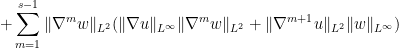
Now we work with the high regularity energy
Arguing as before we have


Using Exercise 2 and Hölder, we may bound this by

Using Sobolev embedding we thus have


By the chain rule, we obtain

(one can work with 


for all
By specialising (7) (or (8)) to the case where 
Proposition 6 Let
be divergence-free. Set
where
be a sequence of divergence-free vector fields converging to
,
be the associated solutions to (1) provided by Corollary 3 (these are well-defined for
norm on
to limits
,
respectively, which solve (1) in a distributional sense.

Proof: We use a variant of Kato’s argument (see also the paper of Bona and Smith for a related technique). It will suffice to show that the 
![{C^0_t H^s_x([0,T] \times {\bf R}^d \rightarrow {\bf R}^d)}](https://s0.wp.com/latex.php?latex=%7BC%5E0_t+H%5Es_x%28%5B0%2CT%5D+%5Ctimes+%7B%5Cbf+R%7D%5Ed+%5Crightarrow+%7B%5Cbf+R%7D%5Ed%29%7D&bg=ffffff&fg=000000&s=0&c=20201002)
Let 
![{v^{(N)}: [0,T] \times {\bf R}^d \rightarrow {\bf R}^d, q^{(N)}}](https://s0.wp.com/latex.php?latex=%7Bv%5E%7B%28N%29%7D%3A+%5B0%2CT%5D+%5Ctimes+%7B%5Cbf+R%7D%5Ed+%5Crightarrow+%7B%5Cbf+R%7D%5Ed%2C+q%5E%7B%28N%29%7D%7D&bg=ffffff&fg=000000&s=0&c=20201002)

![\displaystyle \|u^{(n)}-v^{(N)}\|_{L^\infty_t H^s_x([0,T] \times {\bf R}^d \rightarrow {\bf R}^d)} \lesssim_{s,d} \|u_0^{(n)}- P_{\leq N} u_0\|_{H^s_x({\bf R}^d \rightarrow {\bf R}^d)}](https://s0.wp.com/latex.php?latex=%5Cdisplaystyle++%5C%7Cu%5E%7B%28n%29%7D-v%5E%7B%28N%29%7D%5C%7C_%7BL%5E%5Cinfty_t+H%5Es_x%28%5B0%2CT%5D+%5Ctimes+%7B%5Cbf+R%7D%5Ed+%5Crightarrow+%7B%5Cbf+R%7D%5Ed%29%7D+%5Clesssim_%7Bs%2Cd%7D+%5C%7Cu_0%5E%7B%28n%29%7D-+P_%7B%5Cleq+N%7D+u_0%5C%7C_%7BH%5Es_x%28%7B%5Cbf+R%7D%5Ed+%5Crightarrow+%7B%5Cbf+R%7D%5Ed%29%7D&bg=ffffff&fg=000000&s=0&c=20201002)

Applying the triangle inequality and then taking limit superior, we conclude that
![\displaystyle \limsup_{n,m \rightarrow \infty} \|u^{(n)}-u^{(m)}\|_{L^\infty_t H^s_x([0,T] \times {\bf R}^d \rightarrow {\bf R}^d)} \lesssim_{s,d} \|u_0- P_{\leq N} u_0\|_{H^s_x({\bf R}^d \rightarrow {\bf R}^d)}](https://s0.wp.com/latex.php?latex=%5Cdisplaystyle++%5Climsup_%7Bn%2Cm+%5Crightarrow+%5Cinfty%7D+%5C%7Cu%5E%7B%28n%29%7D-u%5E%7B%28m%29%7D%5C%7C_%7BL%5E%5Cinfty_t+H%5Es_x%28%5B0%2CT%5D+%5Ctimes+%7B%5Cbf+R%7D%5Ed+%5Crightarrow+%7B%5Cbf+R%7D%5Ed%29%7D+%5Clesssim_%7Bs%2Cd%7D+%5C%7Cu_0-+P_%7B%5Cleq+N%7D+u_0%5C%7C_%7BH%5Es_x%28%7B%5Cbf+R%7D%5Ed+%5Crightarrow+%7B%5Cbf+R%7D%5Ed%29%7D+&bg=ffffff&fg=000000&s=0&c=20201002)

But by Plancherel’s theorem and dominated convergence we see that


as 
![\displaystyle \limsup_{n,m \rightarrow \infty} \|u^{(n)}-u^{(m)}\|_{L^\infty_t H^s_x([0,T] \times {\bf R}^d \rightarrow {\bf R}^d)} = 0,](https://s0.wp.com/latex.php?latex=%5Cdisplaystyle++%5Climsup_%7Bn%2Cm+%5Crightarrow+%5Cinfty%7D+%5C%7Cu%5E%7B%28n%29%7D-u%5E%7B%28m%29%7D%5C%7C_%7BL%5E%5Cinfty_t+H%5Es_x%28%5B0%2CT%5D+%5Ctimes+%7B%5Cbf+R%7D%5Ed+%5Crightarrow+%7B%5Cbf+R%7D%5Ed%29%7D+%3D+0%2C&bg=ffffff&fg=000000&s=0&c=20201002)
giving the claim.
Remark 7 Since the sequence
can converge to at most one limit
). In two dimensions, for instance, there is a celebrated theorem of Yudovich that weak solutions to 2D Euler are unique if one has an
bound on the vorticity. In higher dimensions one can also obtain uniqueness results if one assumes that the solution is in a high-regularity space such as
,
Exercise 8 (Continuous dependence on initial data) Let
, where
. The above proposition provides a solution
Remark 9 The continuity result provided by the above exercise is not as strong as in Navier-Stokes, where the solution map is in fact Lipschitz continuous (see e.g., Exercise 43 of Notes 1). In fact for the Euler equations, which is classified as a “quasilinear” equation rather than a “semilinear” one due to the lack of the dissipative term
in the equation, the solution map is not expected to be uniformly continuous on this ball, let alone Lipschitz continuous. See this previous blog post for some more discussion.
Exercise 10 (Maximal Cauchy development) Let
be divergence free. Show that there exists a unique
and unique
,
with the following properties:
- (i) If
is divergence-free and converges to
- (ii) If
, then
as
- (iii) If
Furthermore, show that
do not depend on the particular choice of
for two integers
then the time

We will refine part (iii) of the above exercise in the next section. It is a major open problem as to whether the case 
Remark 11 The condition
, the velocity field
, with the fluctuations being of amplitude
of
where
whose separation at time zero is comparable to the wavelength
of the frequency oscillation. Then the relative velocities of
, and then exhibit more complicated and unpredictable behaviour after that point. Thus the natural time scale
here is
, so one only expects to have a reasonable local well-posedness theory in the regime
On the other hand, if
, the heuristics from the previous notes predict that
The uncertainty principle predicts
, and so
Thus we force the regime (11) to occur if
, but would not expect to have a local theory (at least using the sort of techniques deployed in this section) for
.


Exercise 12 Use similar heuristics to explain the relevance of quantities of the form
that occurs in various places in this section.
Because the solutions constructed in Exercise 10 are limits (in rather strong topologies) of smooth solutions, it is fairly easy to extend estimates and conservation laws that are known for smooth solutions to these slightly less regular solutions. For instance:
Exercise 13 Let
be as in Exercise 10.
- (i) (Energy conservation) Show that
for all
.
- (ii) Show that
for all


Exercise 14 (Vanishing viscosity limit) Let the notation and hypotheses be as in Corollary 3. For each
,
be the solution to (3) with this choice of viscosity and with initial data
and
converge locally uniformly to
.
Exercise 15 (Local existence for forced Euler) Let
be divergence-free, and let
, thus
is smooth and for any
and any integer
and
,
. Show that there exists
Note: one will first need a local existence theory for the forced Navier-Stokes equation. It is also possible to develop forced analogues of most of the other results in this section, but we will not detail this here.


— 2. The Beale-Kato-Majda blowup criterion —
In Exercise 10 we saw that we could continue 

that is to say 


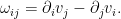
Remark 16 In two dimensions,
and
. As such, it is common in fluid mechanics to refer to the scalar field
as the vorticity, rather than the two form
of the vorticity, and it is common to view
rather than a two-form in this case (actually, to be precise
to scalar functions
, and the relation between the vorticity two-form
in
is given by the relation
for arbitrary vector fields
is the volume form on
The point is that vorticity behaves better under the Euler flow than the full derivative

and applies

If one interchanges 

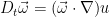
which we can rearrange using the material derivative 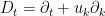

Writing 

The vorticity equation is particularly simple in two and three dimensions:
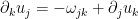
Exercise 17 (Transport of vorticity) Let
- (i) If
, show that
- (ii) If
, show that
where

Remark 18 One can interpret the vorticity equation in the language of differential geometry, which is a more covenient formalism when working on more general Riemann manifolds than
rather than
rather than
). Define the covelocity
-form
where
is the Euclidean metric tensor (in the standard coordinates,
is the Kronecker delta, though
if one uses a different coordinate system). Thus in coordinates,
; the covelocity field is thus the musical isomorphism applied to the velocity field. The vorticity
-form
or in coordinates
The Euler equations can be rearranged as
where
is the Lie derivative along
and
is the modified pressure
If one takes exterior derivatives of both sides of (14) using the basic differential geometry identities
and
, one obtains the vorticity equation
where the Lie derivative for
and so we recover (13) after some relabeling.


We now present the Beale-Kato-Majda condition.
Theorem 19 (Beale-Kato-Majda) Let
- (i) For any
, one has
- (ii) If


The double exponential in (i) is not a typo! It is an open question though as to whether this double exponential bound can be at all improved, even in the simplest case of two spatial dimensions.
We turn to the proof of this theorem. Part (ii) will be implied by part (i), since if 


We would like to convert control on 


Thus, we can recover the derivative 

where one can define 
If the operators 

and the claimed bound (15) would follow from Theorem 1(ii) (with one exponential to spare). Unfortunately, 
for any test function 


If one sets 


But one can calculate using polar coordinates that this expression diverges like 

As it turns out, though, the Gronwall argument used to establish Theorem 1(ii) can just barely tolerate an additional “logarithmic loss” of the above form, albeit at the cost of worsening the exponential term to a double exponential one. The key lemma is the following result that quantifies the logarithmic divergence indicated by the previous calculation, and is similar in spirit to a well known inequality of Brezis and Wainger.
Lemma 20 (Near-boundedness of

The lower order terms 

Proof: By a limiting argument we may assume that

and hence by the triangle inequality we may bound the left-hand side of (17) by
where we omit the domain and range from the function space norms for brevity.
By Bernstein’s inequality we have


Also, from Bernstein and Plancherel we have


and hence by geometric series we have

for any 


for each 
Observe from applying the scaling 


This function is a test function, so
We return now to the proof of (15). We adapt the proof of Proposition 1(i). As in that proposition, we introduce the higher energy
We no longer have the viscosity term as 

Applying (16), (17) one thus has

From Exercise 13 one has

By the chain rule, one then has

and hence by Gronwall’s inequality one has

![\displaystyle \log(2+E(0))) \exp( O_{s,d}( \|\omega \|_{L^1_t L^\infty_x([0,T] \times {\bf R}^d \rightarrow \bigwedge^2 {\bf R}^d)} ) ).](https://s0.wp.com/latex.php?latex=%5Cdisplaystyle++%5Clog%282%2BE%280%29%29%29+%5Cexp%28+O_%7Bs%2Cd%7D%28+%5C%7C%5Comega+%5C%7C_%7BL%5E1_t+L%5E%5Cinfty_x%28%5B0%2CT%5D+%5Ctimes+%7B%5Cbf+R%7D%5Ed+%5Crightarrow+%5Cbigwedge%5E2+%7B%5Cbf+R%7D%5Ed%29%7D+%29+%29.&bg=ffffff&fg=000000&s=0&c=20201002)
The claim (15) follows.
Remark 21 The Beale-Kato-Majda criterion can be sharpened a little bit, by replacing the sup norm
with slightly smaller norms, such as the bounded mean oscillation (BMO) norm of
, basically by improving the right-hand side of Lemma 20 slightly. See for instance this paper of Planchon and the references therein.
Remark 22 An inspection of the proof of Theorem 19 reveals that the same result holds if the Euler equations are replaced by the Navier-Stokes equations; the energy estimates acquire an additional “
We now apply the Beale-Kato-Majda criterion to obtain global well-posedness for the Euler equations in two dimensions:
Theorem 23 (Global well-posedness) Let
be as in Exercise 10. If
.
This theorem will be immediate from Theorem 19 and the following conservation law:
Proposition 24 (Conservation of vorticity distribution) Let
for all
and

Proof: By a limiting argument it suffices to show the claim for 

By another limiting argument we can take
whenever 

![{[0,T] \times {\bf R}^2}](https://s0.wp.com/latex.php?latex=%7B%5B0%2CT%5D+%5Ctimes+%7B%5Cbf+R%7D%5E2%7D&bg=ffffff&fg=000000&s=0&c=20201002)
![{\{ (t,x) \in [0,T] \times {\bf R}^2: \omega_{12}| \geq \varepsilon \}}](https://s0.wp.com/latex.php?latex=%7B%5C%7B+%28t%2Cx%29+%5Cin+%5B0%2CT%5D+%5Ctimes+%7B%5Cbf+R%7D%5E2%3A+%5Comega_%7B12%7D%7C+%5Cgeq+%5Cvarepsilon+%5C%7D%7D&bg=ffffff&fg=000000&s=0&c=20201002)


where we omit explicit dependence on

which one can write as a total derivative
which vanishes thanks to integration by parts and the divergence-free nature of
The above proposition shows that in two dimensions, 
One can adapt this argument to the Navier-Stokes equations:
Exercise 25 Let
be an integer, let
be divergence-free, and let
,
be a maximal Cauchy development to the Navier-Stokes equations with initial data
- (i) Establish the vorticity equation
.
- (ii) Show that
for all
case of this inequality can also be established using the maximum principle for parabolic equations.)
- (iii) Show that
.
Remark 26 There are other ways to establish global regularity for two-dimensional Navier-Stokes (originally due to Ladyzhenskaya); for instance, the
bound on the vorticity in Exercise 25(ii), combined with energy conservation, gives a uniform
bound on the velocity field, which can then be inserted into (the non-periodic version of) Theorem 38 of Notes 1.
Remark 27 If
solve the Euler equations on some time interval
with initial data
, then the time-reversed fields
solve the Euler equations on the reflected interval
with initial data
. Because of this time reversal symmetry, the local and global well-posedness theory for the Euler equations can also be extended backwards in time; for instance, in two dimensions any
. However, the Navier-Stokes equations are very much not time-reversible in this fashion.

23 comments
Comments feed for this article
9 October, 2018 at 9:57 pm
Anonymous
There is no expression in (2).
[Corrected, thanks – T.]
10 October, 2018 at 11:19 am
Anonymous
Dear Terry,
Great post! I have a question on Remark 7. It seems to be an open problem if two dimensional Euler equation has unique weak solution assuming only L^p bound on the vorticity, for p<\infty.
[Oops, I meant here; now corrected. -T]
12 October, 2018 at 12:49 am
yasin şale
Dear Terry,
I would like to read your opinions about the proof of Riemann Hypothesis given by M. Atiyah.
Best regards.
12 October, 2018 at 9:46 pm
Anonymous
Well, I can replace Pro Tao to response your question.According to our observation, Pro Tao seems to be difficult to answer your problem for public,if you meet him in private , he is willing to reply.Because there are many sensitive reasons,although he holds proofs of RH in your hands.On RH,he has 5 ways to approach to RH,every solution seems to constrast to Atiyah’s proof.The second reson , Pro.Tao is the member of Royal committee in England,while Atiyah is also a professor in England.The third reason, he is very old if compare to Tao,so he must respect to Atiyah.According to me,Clay millenium committee will invites Tao to remark Atiyah’sproof,because Pro Tao is the expert on RH,and only members in Clay institue know Atiyah’sproof right or wrong.
12 October, 2018 at 11:39 pm
Anonymous
In order to check Atiyah’s claimed proof of RH, in addition of being expert on RH, it is even more important to be an expert on Todd function and its related functional equations (e.g. Hirzebruch functional equation) on which Atiyah’s claimed proof is based.
13 October, 2018 at 2:13 am
Anonymous
Hello. You must see the comments on the entry “Polymath15, tenth thread: numerics update.”6 September 2018
27 October, 2018 at 5:40 pm
far zeebra
This is mere child’s play. What does the Barrett Series converge to?
The Barrett Series:
1-1/2-(1/2)^2 + (1/2)^3 – (1/2)^4 -(1/2)^5 + (1/2)^6 – (1/2)^7 -(1/2)^8 +(1/2)^9 …
31 October, 2018 at 10:29 pm
YNWA
Dear all, you might be interested in this question concerning the Riemann zeta function on MathOverflow: https://mathoverflow.net/q/314310/130815
2 November, 2018 at 7:32 am
Anonymous
Dear Terry,
Terry Tao-my lovely friend.You have never mett me,but you have a immortal friendliness- a friendliness without border,nothing and anyone can compare it.I am far away with you,I always follow every your step in your jobs.You can image that I am a sattelite.I always support you.In brief, under this great sky,you are lucky to have me,I confirm many times I am the only close friend to you.I know you very well like a clear mirror.No one in the world know that you have good enough on twin prime,navier stokes,birch swinnerton Dyer ,hodge cọnecture,yang mills,collatz conjecture,goldbach,riemann p vs np.But you are stiil silent .You do not want to boast.I like you this point:humble;good virture,patient,gentle,good heart,you have also the sixth sense;you know what someone is doing,but you keep silent.I know that after I write these sentences,many people reject me.Not sense to me.they are still under me with a suppernature head
16 November, 2018 at 2:28 am
Hans
So looking forward for part 4 :-)
21 November, 2018 at 1:05 am
Sergei Ofitserov
Dear Terence Tao! I am sorry by long silence. I am in shock! That no problem of publication! I am know, how to correct your equations outside of Riman hypothesis by theme Nanvier-Stokes. I am is your mate!! We is mutually dependent in following steps. In front transparent simultaneous decision of five sums of millennium! Class N=NP ?? for the time present questionable. I agree able to arrive to you, but how?? My means hardly that’s enough(suffice) only go to airport. But what your position in that situation?? Thanks. Sergei.
15 December, 2018 at 11:44 am
Anonymous
In the proof of Theorem 5, in defining the energy , should the summand be the L^2-norm squared of
  , rather than the dot product of
  and
and  ?
?
[Corrected, thanks – T.]
8 January, 2019 at 3:12 pm
255B, Notes 2: Onsager’s conjecture | What's new
[…] amount of energy at frequencies is at most . On the other hand, by the heuristics in Remark 11 of 254A Notes 3, the time needed for the portion of the solution at frequency to evolve to a higher frequency […]
16 April, 2019 at 7:17 am
Anonymous
Thanks for the excellent notes. A couple of comments:
1) The definition of E^s around the middle of Theorem 5 is a typo (the limit of the sum should be s, and there shouldn’t be a \partial_t on w).
[Corrected, thanks – T.]
2) Aren’t the distributional solutions constructed in Proposition 6 actually strong since \partial_t u \in H^{s-1} ?
[Depends to some extent on what one means by “strong solution”, but yes, there should be enough regularity to verify that the Euler equations hold in a classical sense using classical derivatives here, though in practice this turns out to not be important so long as one knows that the solution is at least the limit of classical solutions.]
16 April, 2019 at 7:28 am
Anonymous
In the proof of Proposition 6, there seems to be a couple of typos: 1) after taking the limsup and using the triangle inequality, v^{(m)} should be u^{(m)} (two instances).
[Corrected, thanks – T.]
2) We only have (and only need) a uniform upper bound on N^{-1} \|P_{\leq N} u_0 \|_{H^{s+1}}
[Actually, I believe we do have convergence to zero in this case also, even though I agree boundedness would already be sufficient. -T]
23 April, 2019 at 10:15 am
Anonymous
In the proof of Lemma 20 (forth and fifth display), d/2-s-1 should be d/2+1-s. Later appearances are correct.
[Corrected, thanks – T.]
18 June, 2021 at 4:52 am
Ning
In the proof of Corollary 3, you used Proposition 2,3 in notes 2 and the Arzela-Ascoli theorem.
It seems that for the Proposition 2, you meant to take , and the assumption of Proposition 2 is satisfied since
  is a subset of
  , which is separable by the fact that its dual
  is separable.
But for the Proposition 3 and Arzela Ascoli theorem, I’m confused about how you take and which version of Arzela Ascoli you used here?
And the result you get from Proposition 3 confused me a lot. Why the weak convergence which you obtained from Proposition 2 is not sufficient to know are solutions to (3) by pairing (3) with test functions, taking limit, and by the smoothness of
  to know they are classical solutions?
19 June, 2021 at 10:38 am
Terence Tao
On each ball , one can use the compact embedding of
 ![L^\infty_t H^{s'}_x([0,T] \times B(0,n))](https://s0.wp.com/latex.php?latex=L%5E%5Cinfty_t+H%5E%7Bs%27%7D_x%28%5B0%2CT%5D+%5Ctimes+B%280%2Cn%29%29&bg=ffffff&fg=545454&s=0&c=20201002) into
into ![L^\infty_t L^\infty_x([0,T] \times B(0,n))](https://s0.wp.com/latex.php?latex=L%5E%5Cinfty_t+L%5E%5Cinfty_x%28%5B0%2CT%5D+%5Ctimes+B%280%2Cn%29%29&bg=ffffff&fg=545454&s=0&c=20201002) (Rellich compactness) and Proposition 3 to obtain a subsequence that converges strongly in
(Rellich compactness) and Proposition 3 to obtain a subsequence that converges strongly in ![L^\infty_t L^\infty_x([0,T] \times B(0,n))](https://s0.wp.com/latex.php?latex=L%5E%5Cinfty_t+L%5E%5Cinfty_x%28%5B0%2CT%5D+%5Ctimes+B%280%2Cn%29%29&bg=ffffff&fg=545454&s=0&c=20201002) for each
for each  . Passing to subsequences once for each
  and then extracting the diagonal sequence (Arzela-Ascoli argument) one obtains a subsequence that converges strongly in
 ![L^\infty_t L^\infty_x([0,T] \times B(0,n))](https://s0.wp.com/latex.php?latex=L%5E%5Cinfty_t+L%5E%5Cinfty_x%28%5B0%2CT%5D+%5Ctimes+B%280%2Cn%29%29&bg=ffffff&fg=545454&s=0&c=20201002) for all
for all  , i.e., converges locally uniformly.
It is also possible to proceed here purely via distributional limits as you suggest since the weak-strong uniqueness one needs is indeed easy at this high level of regularity.
18 June, 2021 at 5:32 am
Ning
In Remark 4, you said that `In the presence of a boundary, we cannot freely differentiate in space as casually as we have been doing above’
Is that because we do not have the prior bound like that in Theorem 1, then we could not get the desired boundedness? I did not quite understand what you mean by casually differentiating in space.
19 June, 2021 at 10:42 am
Terence Tao
Once one is working in a domain with boundary, then one has to be careful because there are now several inequivalent notions of derivative one can use. For instance, consider the constant function
  on
on  . Naively this function has gradient zero. But if instead one extends this function by zero to all of
  to obtain the indicator function
  then the (weak) gradient of this function is instead a (vector-valued) distribution on the boundary
  . Related to this, there are now several inequivalent Sobolev spaces
  , etc. that one can define on
  , associated with different boundary conditions, and partial differentiation operations (such as the Laplacian) do not necessarily preserve these boundary conditions. (Also, it is not always true that test functions
  are dense in these spaces, which causes additional complications.) The book by Constantin and Foias on Navier-Stokes equations for instance treats these issues in some detail.
19 October, 2021 at 3:44 pm
Kevin Hu
Hi Dr. Tao, for the expression of \p_tE(t) right below the proof of Lemma 20, I think the indices are inconsistent.
[Corrected, thanks – T.]
25 October, 2021 at 3:43 am
Daniel Eriksson
Before Remark 21, when we apply Gronwall shouldn’t there be an exponential factor on both terms, exp(O_{s,d}||omega||)_{L1Linf})(log(2+E(0))+T(||u_0||_{L^2}+1))?
[Corrected, thanks – T.]
27 October, 2021 at 7:55 am
Lorenzo Pompili
Dear Professor Tao, in the proof of Lemma 20: there should be
  instead of
  (same thing for the very next sentence).
 a generic function in order to state and prove the estimate, but
  is also the name of the test function that appears in the definition of the Littlewood-Paley projections. I would suggest to use another symbol, as the two appear quite close to each other and that can generate some confusion.
I think there is a typo in the definition of
Also, in formula (18) and right after that, I think you are calling
[Corrected, thanks – T.]