254A, Notes 2: Weak solutions of the Navier-Stokes equations

2 October, 2018 in 254A - Incompressible fluid equations, math.AP, math.CA | Tags: compactness, distributions, Navier-Stokes equations, weak solutions | by Terence Tao

In the previous set of notes we developed a theory of “strong” solutions to the Navier-Stokes equations. This theory, based around viewing the Navier-Stokes equations as a perturbation of the linear heat equation, has many attractive features: solutions exist locally, are unique, depend continuously on the initial data, have a high degree of regularity, can be continued in time as long as a sufficiently high regularity norm is under control, and tend to enjoy the same sort of conservation laws that classical solutions do. However, it is a major open problem as to whether these solutions can be extended to be (forward) global in time, because the norms that we know how to control globally in time do not have high enough regularity to be useful for continuing the solution. Also, the theory becomes degenerate in the inviscid limit ${\nu \rightarrow 0}$ .

However, it is possible to construct “weak” solutions which lack many of the desirable features of strong solutions (notably, uniqueness, propagation of regularity, and conservation laws) but can often be constructed globally in time even when one us unable to do so for strong solutions. Broadly speaking, one usually constructs weak solutions by some sort of “compactness method”, which can generally be described as follows.

Construct a sequence of “approximate solutions” to the desired equation, for instance by developing a well-posedness theory for some “regularised” approximation to the original equation. (This theory often follows similar lines to those in the previous set of notes, for instance using such tools as the contraction mapping theorem to construct the approximate solutions.)
Establish some uniform bounds (over appropriate time intervals) on these approximate solutions, even in the limit as an approximation parameter is sent to zero. (Uniformity is key; non-uniform bounds are often easy to obtain if one puts enough “mollification”, “hyper-dissipation”, or “discretisation” in the approximating equation.)
Use some sort of “weak compactness” (e.g., the Banach-Alaoglu theorem, the Arzela-Ascoli theorem, or the Rellich compactness theorem) to extract a subsequence of approximate solutions that converge (in a topology weaker than that associated to the available uniform bounds) to a limit. (Note that there is no reason a priori to expect such limit points to be unique, or to have any regularity properties beyond that implied by the available uniform bounds..)
Show that this limit solves the original equation in a suitable weak sense.

The quality of these weak solutions is very much determined by the type of uniform bounds one can obtain on the approximate solution; the stronger these bounds are, the more properties one can obtain on these weak solutions. For instance, if the approximate solutions enjoy an energy identity leading to uniform energy bounds, then (by using tools such as Fatou’s lemma) one tends to obtain energy inequalities for the resulting weak solution; but if one somehow is able to obtain uniform bounds in a higher regularity norm than the energy then one can often recover the full energy identity. If the uniform bounds are at the regularity level needed to obtain well-posedness, then one generally expects to upgrade the weak solution to a strong solution. (This phenomenon is often formalised through weak-strong uniqueness theorems, which we will discuss later in these notes.) Thus we see that as far as attacking global regularity is concerned, both the theory of strong solutions and the theory of weak solutions encounter essentially the same obstacle, namely the inability to obtain uniform bounds on (exact or approximate) solutions at high regularities (and at arbitrary times).

For simplicity, we will focus our discussion in this notes on finite energy weak solutions on ${{\bf R}^d}$ . There is a completely analogous theory for periodic weak solutions on ${{\bf R}^d}$ (or equivalently, weak solutions on the torus ${({\bf R}^d/{\bf Z}^d)}$ which we will leave to the interested reader.

In recent years, a completely different way to construct weak solutions to the Navier-Stokes or Euler equations has been developed that are not based on the above compactness methods, but instead based on techniques of convex integration. These will be discussed in a later set of notes.

— 1. A brief review of some aspects of distribution theory —

We have already been using the concept of a distribution in previous notes, but we will rely more heavily on this theory in this set of notes, so we pause to review some key aspects of the theory. A more comprehensive discussion of distributions may be found in this previous blog post. To avoid some minor subtleties involving complex conjugation that are not relevant for this post, we will restrict attention to real-valued (scalar) distributions here. (One can then define vector-valued distributions (taking values in a finite-dimensional vector space) as a vector of scalar-valued distributions.)

Let us work in some non-empty open subset ${U}$ of a Euclidean space ${{\bf R}^d}$ (which may eventually correspond to space, time, or spacetime). We recall that ${C^\infty_c(U \rightarrow {\bf R})}$ is the space of (real-valued) test functions ${\phi: U \rightarrow {\bf R}}$ . It has a rather subtle topological structure (see previous notes) which we will not detail here. A (real-valued) distribution ${\lambda}$ on ${U}$ is a continuous linear functional ${\phi \mapsto \langle \lambda, \phi \rangle}$ from test functions ${\phi \in C^\infty_c(U \rightarrow {\bf R})}$ to the reals ${{\bf R}}$ . (This pairing ${\langle \lambda, \phi \rangle}$ may also be denoted ${\langle \phi,\lambda \rangle}$ or ${\lambda(\phi)}$ in other texts.) There are two basic examples of distributions to keep in mind:

Any locally integrable function ${f \in L^1_{loc}(U \rightarrow {\bf R})}$ gives rise to a distribution (which by abuse of notation we also call ${f}$ ) by the formula ${\langle f, \phi \rangle := \int_{U} f(x) \phi(x)\ dx}$ .
Any Radon measure ${\mu \in M(U)}$ gives rise to a distribution (which we will again call ${\mu}$ ) by the formula ${\langle \mu, \phi \rangle = \int_{U} \phi(x)\ d\mu(x)}$ . For instance, if ${x_0 \in U}$ , the Dirac mass ${\delta_{x_0}}$ at ${x_0}$ is a distribution with ${\langle \delta_{x_0}, \phi \rangle = \phi(x_0)}$ .

Two distributions ${\lambda, \eta}$ are equal in the sense of distributions of ${\langle \lambda, \phi \rangle = \langle \eta, \phi \rangle}$ for all ${\phi \in C^\infty_c(U \rightarrow {\bf R})}$ . For instance, it is not difficult to show that two locally integrable functions are equal in the sense of distributions if and only if they agree almost everywhere, and two Radon measures are equal in the sense of distributions if and only if they are identical.

As a general principle, any “linear” operation that makes sense for “nice” functions (such as test functions) can also be defined for distributions, but any “nonlinear” operation is unlikely to be usefully defined for arbitrary distributions (though it may still be a good concept to use for distributions with additional regularity). For instance, one can take a partial derivative ${\partial_i \lambda}$ (known as the weak derivative) of any distribution ${\lambda}$ by the definition

$\displaystyle \langle \partial_i \lambda, \phi \rangle := - \langle \lambda, \partial_i \phi \rangle$

for all ${\phi \in C^\infty_c(U \rightarrow {\bf R})}$ . Note that this definition agrees with the “strong” or “classical” notion of a derivative when ${\lambda}$ is a smooth function, thanks to integration by parts. Similarly, if ${f \in C^\infty(U \rightarrow {\bf R})}$ is smooth, one can define the product distribution ${f\lambda = \lambda f}$ by the formula

$\displaystyle \langle f \lambda, \phi \rangle := \langle \lambda, f \phi \rangle$

for all ${\phi \in C^\infty_c(U \rightarrow {\bf R})}$ . One can also take linear combinations of two distributions ${\lambda, \eta}$ in the usual fashion, thus

$\displaystyle \langle a \lambda + b \nu, \phi \rangle = a \langle \lambda, \phi \rangle + b \langle \nu, \phi \rangle$

for all ${a,b \in {\bf R}}$ and ${\phi \in C^\infty_c(U \rightarrow {\bf R})}$ .

Exercise 1 Let ${U}$ be a connected open subset of ${{\bf R}^d}$ . Let ${\lambda}$ be a distribution on ${U}$ such that ${\partial_i \lambda = 0}$ in the sense of distributions for all ${i=1,\dots,d}$ . Show that ${\lambda}$ is a constant, that is to say there exists ${c \in {\bf R}}$ such that ${\lambda = c}$ in the sense of distributions.

A sequence of distributions ${\lambda_n}$ is said to converge in the weak-* sense or converge in the sense of distributions to another distribution ${\lambda}$ if one has

$\displaystyle \langle \lambda_n, \phi \rangle \rightarrow \langle \lambda, \phi \rangle$

as ${n \rightarrow \infty}$ for every test function ${\phi}$ ; in this case we write ${\lambda_n \rightharpoonup^* \lambda}$ . This notion of convergence is sometimes referred to also as weak convergence (and one writes ${\lambda_n \rightharpoonup \lambda}$ instead of ${\lambda_n \rightharpoonup^* \lambda}$ ), although there is a subtle distinction between weak and weak-* convergence in non-reflexive spaces and so I will try to avoid this terminology (though in many cases one will be working in a reflexive space in which there is no distinction).

The linear operations alluded to above tend to be continuous in the distributional sense. For instance, it is easy to see that if ${\lambda_n \rightharpoonup^* \lambda}$ , then ${\partial_i \lambda_n \rightharpoonup^* \partial_i \lambda}$ for all ${i=1,\dots,d}$ , and ${f \lambda_n \rightharpoonup^* f \lambda}$ for any smooth ${f}$ ; similarly, if ${\lambda_n \rightharpoonup^* \lambda}$ , ${\mu_n \rightharpoonup^* \mu}$ , and ${a_n \rightarrow a}$ , ${b_n \rightarrow b}$ are sequences of real numbers, then ${a_n \lambda_n + b_n \mu_n \rightharpoonup^* a \lambda + b \mu}$ .

Suppose that one places a norm or seminorm ${\| \|_X}$ on ${C^\infty_c(U \rightarrow {\bf R})}$ . Then one can define a subspace ${X^*}$ of the space of distributions, defined to be the space of all distributions ${\lambda}$ for which the norm

$\displaystyle \| \lambda \|_{X^*} := \sup_{\phi \in C^\infty_c(U \rightarrow {\bf R}): \|\phi \|_X \leq 1} |\langle \lambda, \phi \rangle|$

is finite. For instance, if ${X}$ is the ${L^p}$ norm for some ${1 \leq p < \infty}$ , then ${X^*}$ is just the dual space ${L^{p'}(U \rightarrow {\bf R})}$ (with the (equivalence classes of) locally integrable functions in ${L^{p'}(U \rightarrow {\bf R})}$ identified with distributions as above).

We have the following version of the Banach-Alaoglu theorem which allows us to easily create sequences that converge in the sense of distributions:

Proposition 2 (Variant of Banach-Alaoglu) Suppose that ${\| \|_X}$ is a norm or seminorm on ${C^\infty_c(U \rightarrow {\bf R})}$ which makes the space ${C^\infty_c(U \rightarrow {\bf R})}$ separable. Let ${\lambda_n}$ be a bounded sequence in ${X^*}$ . Then there is a subsequence of the ${\lambda_n}$ which converges in the sense of distributions to a limit ${\lambda \in X^*}$ .

Proof: By hypothesis, there is a constant ${C}$ such that

$\displaystyle |\langle \lambda_n, \phi \rangle| \leq C \|\phi \|_X \ \ \ \ \ (1)$

for all ${\phi \in C^\infty_c(U \rightarrow {\bf R})}$ . For each given ${\phi}$ , we may thus pass to a subsequence of ${\lambda_n}$ such that ${\langle \lambda_n, \phi \rangle}$ converges to a limit. Passing to a subsequence a countably infinite number of times and using the Arzelá-Ascoli diagonalisation trick, we can thus find a dense subset ${{\mathcal D}}$ of ${C^\infty_c(U \rightarrow {\bf R})}$ (using the ${\| \|_X}$ metric) and a subsequence ${\lambda_{n_j}}$ of the ${\lambda_n}$ such that the limit ${\lim_{j \rightarrow \infty} \langle \lambda_{n_j}, \phi \rangle}$ exists for every ${\phi \in {\mathcal D}}$ , and hence for every ${\phi \in C^\infty_c({\bf R}^d)}$ by a limiting argument and (1). If one then defines ${\lambda}$ to be the function

$\displaystyle \langle \lambda,\phi \rangle := \lim_{j \rightarrow \infty} \langle \lambda_{n_j}, \phi \rangle,$

then one can verify that ${\lambda}$ is a distribution, and by (1) we will have ${\lambda \in X^*}$ . By construction, ${\lambda_{n_j}}$ converges in the sense of distributions to ${\lambda}$ , and we are done. $\Box$

It is important to note that there is no uniqueness claimed for ${\lambda}$ ; while any given subsequence of the ${\lambda_n}$ can have at most one limit ${\lambda}$ , it is certainly possible for different subsequences to converge to different limits. Also, the proposition only applies for spaces ${X^*}$ that have preduals ${X}$ ; this covers many popular function spaces, such as ${L^p({\bf R}^d \rightarrow {\bf R})}$ spaces for ${1 < p \leq \infty}$ , but omits endpoint spaces such as ${L^1({\bf R}^d \rightarrow {\bf R})}$ or ${C_0({\bf R}^d \rightarrow {\bf R})}$ . (For instance, approximations to the identity are uniformly bounded in ${L^1}$ , but converge weakly to a Dirac mass, which lies outside of ${L^1}$ .)

From definition we see that if ${\lambda_n \rightharpoonup^* \lambda}$ , then we have the Fatou-type lemma

$\displaystyle \| \lambda \|_{X^*} \leq \liminf_{n \rightarrow \infty} \| \lambda_n \|_{X^*}. \ \ \ \ \ (2)$

Thus, upper bounds on the approximating distributions ${\lambda_n}$ are usually inherited by their limit ${\lambda}$ . However, it is essential to be aware that the same is not true for lower bounds; there can be “loss of mass” in the limit. The following four examples illustrate some key ways in which this can occur:

(Escape to spatial infinity) If ${\phi \in C^\infty_c({\bf R}^d \rightarrow {\bf R})}$ is a non-zero test function, and ${x_n}$ is a sequence in ${{\bf R}^d}$ going to infinity, then the translations ${x \mapsto \phi(x-x_n)}$ of ${\phi}$ converge in the sense of distributions to zero, even though they will not go to zero in many function space norms (such as ${L^p}$ ).
(Escape to frequency infinity) If ${\phi \in C^\infty_c({\bf R}^d \rightarrow {\bf R})}$ is a non-zero test function, and ${\xi_n}$ is a sequence in ${{\bf R}^d}$ going to infinity, then the modulations ${x \mapsto \cos(2\pi \xi_n \cdot x) \phi(x)}$ of ${\phi}$ converge in the sense of distributions to zero (cf. the Riemann-Lebesgue lemma), even though they will not go to zero in many function space norms (such as ${L^p}$ ).
(Escape to infinitely fine scales) If ${\phi \in C^\infty_c({\bf R}^d \rightarrow {\bf R})}$ , ${\lambda_n}$ is a sequence of positive reals going to infinity, and ${\alpha < d}$ , then the sequence ${x \mapsto \lambda_n^\alpha \phi(\lambda_n x)}$ converges in the sense of distributions to zero, but will not go to zero in several function space norms (e.g. ${L^p}$ with ${p \geq d/\alpha}$ ).
(Escape to infinitely coarse scales) If ${\phi \in C^\infty_c({\bf R}^d \rightarrow {\bf R})}$ , ${\lambda_n}$ is a sequence of positive reals going to zero, and ${\alpha > 0}$ , then the sequence ${x \mapsto \lambda_n^\alpha \phi(\lambda_n x)}$ converges in the sense of distributions to zero, but will not go to zero in several function space norms (e.g. ${L^p}$ with ${p \leq d/\alpha}$ ).

Related to this loss of mass phenomenon is the important fact that the operation of pointwise multiplication is generally not continuous in the distributional topology: ${\lambda_n \rightharpoonup^* \lambda}$ and ${\eta_n \rightharpoonup^* \eta}$ does not necessarily imply ${\lambda_n \eta_n \rightharpoonup^* \lambda \eta}$ in general (in fact in many cases the products ${\lambda_n \eta_n}$ or ${\lambda \eta}$ might not even be well-defined). For instance:

Using the escape to frequency infinity example, the functions ${x \mapsto \cos(\xi_n \cdot x) \phi(x)}$ converge in the sense of distributions to zero, but their squares ${x \mapsto (\cos(\xi_n \cdot x) \phi(x))^2}$ instead converge in the sense of distributions to ${x \mapsto \frac{1}{2} \phi^2(x)}$ , as can be seen from the double angle formula ${\cos(\theta)^2 = \frac{1}{2} + \frac{1}{2} \cos(2\theta)}$ .
Using the escape to infinitely fine scales example, the functions ${x \mapsto \lambda_n^\alpha \phi(\lambda_n x)}$ converge in the sense of distributions to zero, but their squares ${x \mapsto (\lambda_n^\alpha \phi(\lambda_n x))^2}$ will not if ${\alpha > d/2}$ .

This lack of continuity of multiplication means that one has to take a non-trivial amount of care when applying the theory of distributions to nonlinear PDE; a sufficiently careless regard for this issue (or more generally, treating distribution theory as some sort of “magic wand“) is likely to lead to serious errors in one’s arguments.

One way to recover continuity of pointwise multiplication is to somehow upgrade distributional convergence to stronger notions of convergence. For instance, from Hölder’s inequality one sees that if ${\lambda_n}$ converges strongly to ${\lambda}$ in ${L^p(U \rightarrow {\bf R})}$ (thus ${\lambda_n}$ and ${\lambda}$ both lie in ${L^p}$ , and ${\| \lambda_n - \lambda \|_{L^p}}$ goes to zero), and ${\eta_n}$ converges strongly to ${\eta}$ in ${L^q(U \rightarrow {\bf R})}$ , then ${\lambda_n \eta_n}$ will converge strongly in ${L^r(U \rightarrow {\bf R})}$ to ${\lambda \eta}$ , where ${\frac{1}{r} = \frac{1}{p} + \frac{1}{q}}$ .

One key way to obtain strong convergence in some norm is to obtain uniform bounds in an even stronger norm – so strong that the associated space embeds compactly in the space associated to the original norm. More precisely

Proposition 3 (Upgrading to strong convergence) Let ${\| \|_X, \| \|_Y}$ be two norms on ${C^\infty_c(U \rightarrow {\bf R})}$ , with associated spaces ${X^*, Y^*}$ of distributions. Suppose that ${X^*}$ embeds compactly into ${Y^*}$ , that is to say the closed unit ball in ${X^*}$ is a compact subset of ${Y^*}$ . If ${\lambda_n}$ is a bounded sequence in ${X^*}$ that converges in the sense of distributions to a limit ${\lambda}$ , then ${\lambda_n}$ converges strongly in ${Y^*}$ to ${\lambda}$ as well.

Proof: By the Urysohn subsequence principle, it suffices to show that every subsequence of ${\lambda_n}$ has a further subsequence that converges strongly in ${Y^*}$ to ${\lambda}$ . But by the compact embedding of ${X^*}$ into ${Y^*}$ , every subsequence of ${\lambda_n}$ has a further subsequence that converges strongly in ${Y^*}$ to some limit ${\lambda'}$ , and hence also in the sense of distributions to ${\lambda'}$ by definition of the ${Y^*}$ norm. But thus subsequence also converges in the sense of distributions to ${\lambda}$ , and hence ${\lambda = \lambda'}$ , and the claim follows. $\Box$

— 2. Simple examples of weak solutions —

We now study weak solutions for some very simple equations, as a warmup for discussing weak solutions for Navier-Stokes.

We begin with an extremely simple initial value problem, the ODE

$\displaystyle \partial_t u = f$

on a half-open time interval ${[0,T)}$ with ${0 < T \leq \infty}$ , with initial condition ${u_0 = u(0)}$ , where ${f: [0,T) \rightarrow {\bf R}}$ and ${u_0 \in {\bf R}}$ given and ${u: [0,T) \rightarrow {\bf R}}$ is the unknown. Of course, when ${f,u}$ are smooth, then the fundamental theorem of calculus gives the unique solution

$\displaystyle u(t) = u_0 + \int_0^t f(s)\ ds \ \ \ \ \ (3)$

for ${t \in [0,T)}$ . If one integrates the identity ${\partial_t u - f = 0}$ against a test function ${\phi \in C^\infty_c((-\infty,T))}$ (that is to say, one multiplies both sides of this identity by ${\phi}$ and then integrates) on ${[0,T)}$ , one obtains

$\displaystyle \int_0^T (\partial_t u - f)(s) \phi(s)\ ds = 0$

which upon integration by parts and rearranging gives

$\displaystyle - \langle u, \partial_t \phi \rangle = \langle u_0 \delta_0, \phi \rangle + \langle f, \phi \rangle$

where we extend ${u, f}$ by zero to the open set ${(-\infty,T)}$ . Thus, we have

$\displaystyle \partial_t u = u_0 \delta_0 + f \ \ \ \ \ (4)$

in the sense of distributions (on ${(-\infty,T)}$ ). More generally, if ${u,f}$ are locally integrable functions on ${[0,T)}$ , we say that ${u}$ is a weak solution to the initial value problem ${\partial_t u = f, u(0) =u_0}$ if (4) holds in the sense of distributions on ${(-\infty,T)}$ . Thanks to the fundamental theorem of calculus for locally integrable functions, we still recover the unique solution (3):

Exercise 4 Let ${u,f: [0,T) \rightarrow {\bf R}}$ be locally integrable functions (extended by zero to all of ${{\bf R}}$ ), and let ${u_0 \in {\bf R}}$ . Show that the following are equivalent:

(i) ${u}$ is a weak solution to the initial value problem ${\partial_t u = f, u(0) = u_0}$ in the sense that (4) holds in the sense of distributions on ${(-\infty,T)}$ .
(ii) One has (3) for almost all ${t \in [0,T)}$ .

Now let ${V}$ be a finite dimensional vector space, let ${F: V \rightarrow V}$ be a continuous function, let ${u_0 \in V}$ , and consider the initial value problem

$\displaystyle \partial_t u = F(u); \quad u(0) = u_0 \ \ \ \ \ (5)$

on some forward time interval ${[0,T)}$ . The Picard existence theorem lets us construct such solutions when ${F}$ is Lipschitz continuous and ${T}$ is small enough, but now we are merely requiring ${F}$ to be continuous and not necessarily Lipschitz. As in the preceding case, we introduce the notion of a weak solution. If ${u}$ is locally bounded (and measurable) on ${[0,T)}$ , then ${F(u)}$ will be locally integrable on ${[0,T)}$ ; we then extend ${u, F(u)}$ by zero to be distributions on ${(-\infty,T)}$ , and we say that ${u}$ is a weak solution to (5) if one has

$\displaystyle \partial_t u = u_0 \delta_0 + F(u)$

in the sense of distributions on ${(-\infty,T)}$ , or equivalently that one has the identity

$\displaystyle - \int_0^T u(s) \partial_t \phi(s)\ ds = u_0 \phi(0) + \int_0^T F(u(s)) \phi(s)\ ds$

for all test functions ${\phi}$ compactly supported in ${(-\infty,T)}$ . In this simple ODE setting, the notion of a weak solution coincides with stronger notions of solutions:

Exercise 5 Let ${V}$ be finite dimensional, let ${F: V \rightarrow V}$ be continuous, let ${u_0 \in V}$ , and let ${u: [0,T) \rightarrow V}$ be locally bounded and measurable. Show that the following are equivalent:

(i) (Weak solution) ${u}$ is a weak solution to (5) on ${[0,T)}$ .
(ii) (Mild solution) After modification on a set of measure zero, ${u}$ is continuous and ${u(t) = u_0 + \int_0^t F(u(s))\ ds}$ for all ${t \in [0,T)}$ .
(iii) (Classical solution) After modification on a set of measure zero, ${u}$ is continuously differentiable and obeys (5) for all ${t \in [0,T)}$ .

In particular, if the ODE initial value problem (5) exhibits finite time blowup for its (unique) classical solution, then it will also do so for weak solutions (with exactly the same blouwp time). This will be in contrast with the situation for PDE, in which it is possible for weak solutions to persist beyond the time in which classical solutions exist.

Now we give a compactness argument to produce weak solutions (which will then be classical solutions, by the above exercise):

Proposition 6 (Weak existence) Let ${V}$ be a finite dimensional vector space, let ${R>0}$ , let ${u_0 \in \overline{B(0,R)}}$ , and let ${F: V \rightarrow V}$ be a continuous function. Let ${T>0}$ be the time
$\displaystyle T := \frac{R}{\sup_{u \in \overline{B(0,2R)}} \|F(u)\|_V}.$
Then there exists a continuously differentiable solution ${u: [0,T) \rightarrow \overline{B(0,2R)}}$ to the initial value problem (5) on ${[0,T)}$ .

Proof: By construction, we have

$\displaystyle \sup_{u \in \overline{B(0,2R)}} \|F(u)\|_V = \frac{R}{T}.$

Using the Weierstrass approximation theorem (or Stone-Weierstrass theorem), we can express ${F}$ on ${\overline{B(0,2R)}}$ as the uniform limit of Lipschitz continuous functions ${F_n: \overline{B(0,2R)} \rightarrow V}$ , such that

$\displaystyle \sup_{u \in \overline{B(0,2R)}} \|F_n(u)\|_V \leq \frac{R}{T}. \ \ \ \ \ (6)$

for all ${n}$ ; we can then extend ${F_n}$ in a Lipschitz continuous fashion to all of ${V}$ . (The Lipschitz constant of ${F_n}$ is permitted to diverge to infinity as ${n \rightarrow \infty}$ ). We can then apply the Picard existence theorem (Theorem 8 of Notes 1), for each ${n}$ we have a (continuously differentiable) maximal Cauchy development ${u_n: [0,T_n) \rightarrow V}$ of the initial value problem

$\displaystyle \partial_t u_n = F_n(u_n); \quad u_n(0) = u_0 \ \ \ \ \ (7)$

with ${\|u_n(t)\|_V \rightarrow \infty}$ as ${t \rightarrow T_n^-}$ if ${T_n}$ is finite. (We could also solve the ODE backwards in time, but will not need to do so here.) We now claim that ${T_n \geq T}$ , and furthermore that one has the uniform bound

$\displaystyle \|u_n(t)\|_V \leq 2R \ \ \ \ \ (8)$

for all ${n}$ and all ${0 \leq t \leq T}$ . Indeed, if this were not the case then by continuity (and the fact that ${\|u_n(0)\|_V = \|u_0\|_V \leq R < 2R}$ ) there would be some ${n}$ and some ${0 < t_n < \min(T,T_n)}$ such that ${\|u_n(t_n)\|_V = 2R}$ , and ${\| u_n(t)\|_V < 2R}$ for all ${0 \leq t < t_n}$ . But then by the fundamental theorem of calculus and the triangle inequality (and (6)) we have

$\displaystyle 2R = \| u_n(t_n) \|_V \leq \|u_0\|_V + \int_0^{t_n} \| F(u_n(s))\|_V\ ds$

$\displaystyle \leq R + t_n \sup_{u \in \overline{B(0,2R)}} \|F_n(u)\|_V$

$\displaystyle < 2R,$

a contradiction. Thus we have (8) for all ${n}$ and ${0 \leq t \leq T}$ , so ${u_n}$ takes values in ${\overline{B(0,2R)}}$ on ${[0,T]}$ . Applying (7), (6) we conclude that

$\displaystyle \| \partial_t u_n(t) \|_V \leq \frac{R}{T}$

for all ${n}$ and all ${0 \leq t \leq T}$ ; in particular, the ${u_n}$ are uniformly Lipschitz continuous and uniformly bounded on ${[0,T]}$ . Applying the Arzelá-Ascoli theorem, we can then pass to a subsequence in which the ${u_n}$ converge uniformly on ${[0,T)}$ to a limit ${u}$ , which then also takes values in ${\overline{B(0,2R)}}$ . (Alternatively, one could use Proposition 2 to have ${u_n}$ converge in the sense of distributions, followed by Proposition 3 to upgrade to uniform convergence.) As ${F_n}$ converges uniformly to ${F}$ on ${\overline{B(0,2R)}}$ , we conclude that ${F_n(u_n)}$ converges uniformly to ${F(u)}$ on ${[0,T)}$ . Since we have

$\displaystyle \partial_t u_n = u_0 \delta_0 + F_n(u_n)$

in the sense of distributions (extending ${u_n}$ , ${F_n(u_n)}$ by zero to ${(-\infty,T)}$ ), we can take distributional limits and conclude that

$\displaystyle \partial_t u = u_0 \delta_0 + F(u)$

in the sense of distributions, which by Exercise 5 shows that ${u: [0,T) \rightarrow \overline{B(0,2R)}}$ is a continuously differentiable solution to the initial value problem (5) as required. $\Box$

In contrast to the Picard theory when ${F}$ is Lipschitz, Proposition 6 does not assert any uniqueness of the solution ${u}$ to the initial value problem (5). And in fact uniqueness often fails once the Lipschitz hypothesis is dropped! Consider the simple example of the scalar initial value problem

$\displaystyle \partial_t u = |u|^{1/2}; \quad u(0) = 0$

on ${[0,+\infty)}$ , so the nonlinearity here is the continuous, but not Lipschitz continuous, function ${u \mapsto |u|^{1/2}}$ . Clearly the zero function ${u(0) = 0}$ is a solution to this ODE. But so is the function ${u(t) := t^2/4}$ . In fact there are a continuum of solutions: for any ${t_0 \geq 0}$ , the function ${u(t) := \max(t-t_0,0)^2/4}$ is a solution. Proposition 6 will select one of these solutions, but the precise solution selected will depend on the choice of approximating functions ${F_n}$ :

Exercise 7 Let ${t_0>0}$ . For each ${n}$ , let ${F_n: {\bf R} \rightarrow {\bf R}}$ denote the function
$\displaystyle F_n(u) := \left( \max( |u|-\frac{1}{n}, 0 ) + \frac{1}{n^2 t_0^2} \right)^{1/2}.$

(i) Show that each ${F_n}$ is Lipschitz continuous, and the ${F_n}$ converge uniformly to the function ${F(u) := |u|^{1/2}}$ as ${n \rightarrow \infty}$ .
(ii) Show that the solution ${u_n: [0,+\infty) \rightarrow {\bf R}}$ to the initial value problem ${\partial_t u_n = F_n(u_n), u_n(0) = 0}$ is given by
$\displaystyle u_n(t) = \frac{t}{nt_0}$
for ${0 \leq t \leq t_0}$ and
$\displaystyle u_n(t) = \frac{1}{n} - \frac{1}{n^2 t_0^2} + \frac{ \left( t - t_0 + \frac{2}{nt_0} \right)^2}{4}$
for ${t \geq t_0}$ .
(iii) Show that as ${n \rightarrow \infty}$ , ${u_n}$ converges locally uniformly to the function ${t \mapsto \max(t-t_0,0)^2/4}$ .

Now we give a simple example of a weak solution construction for a PDE, namely the linear transport equation

$\displaystyle \partial_t u(t,x) + v(x) \partial_x u(t,x) = 0; \quad u(0,x) = u_0(x) \ \ \ \ \ (9)$

where the initial data ${u_0: {\bf R} \rightarrow {\bf R}}$ and a position-dependent velocity field ${v: {\bf R} \rightarrow {\bf R}}$ is given, and ${u: [0,+\infty) \times {\bf R} \rightarrow {\bf R}}$ is the unknown field.

Suppose for the moment that ${u_0, v, u}$ are smooth, with ${v}$ bounded. Then one can solve this problem using the method of characteristics. For any ${x_0 \in {\bf R}}$ , let ${\Phi(t)(x_0)}$ denote the solution to the initial value problem

$\displaystyle \partial_t \Phi(t)(x_0) = v(\Phi(t)(x_0)); \quad \Phi(0)(x_0) = x_0. \ \ \ \ \ (10)$

The Picard existence theorem gives us a smooth maximal Cauchy development ${t \mapsto \Phi(t)(x_0)}$ for this problem; as ${v}$ is bounded, this development cannot go to infinity in finite time (either forward or backwards in time), and so the solution is global. Thus we have a well-defined map ${\Phi(t): {\bf R} \rightarrow {\bf R}}$ for each time ${t \in {\bf R}}$ . In fact we can say more:

Exercise 8 Let the assumptions be as above.

(i) Show the semigroup property ${\Phi(t_1 + t_2) = \Phi(t_1) \circ \Phi(t_2)}$ for all ${t_1,t_2 \in {\bf R}}$ .
(ii) Show that ${\Phi(t)}$ is a homeomorphism for each ${t \in {\bf R}}$ .
(iii) Show that for every ${t}$ , ${\Phi(t)}$ is differentiable, and the derivative ${\partial_x \Phi(t)}$ obeys the linear initial value problem
$\displaystyle \partial_t \partial_x \Phi(t)(x) = v'(\Phi(t)(x)) \partial_x \Phi(t)(x); \quad \partial_x \Phi(0)(x) = 1.$
(Hint: while this system formally can be obtained by differentiating (10) in ${x_0}$ , this formal differentiation requires rigorous justification. One can for instance proceed by first principles, showing that the Newton quotients ${\frac{\Phi(t)(x+h)-\Phi(t)(x)}{h}}$ approximately obey this equation, and then using a Gronwall inequality argument to compare this approximate solution to an exact solution.)
(iv) Show that ${\Phi(t)}$ is a ${C^1}$ diffeomorphism for each ${t}$ ; that is to say, ${\Phi(t)}$ and its inverse are both continuously differentiable.
(v) Show that ${\Phi(t)}$ is a smooth diffeomorphism (that is to say ${\Phi(t)}$ and its inverse are both smooth). (Caution: one may require a bit of planning to avoid the proof becoming extremely long and tedious.)

From (10) and the chain rule we have the identity

$\displaystyle \frac{d}{dt} u( t, \Phi(t)(x) ) = (\partial_t u + v \partial_x u)( t, \Phi(t)(x) )$

for any smooth function ${u}$ (cf. the material derivative used in Notes 0). Thus, one can rewrite the initial value problem (9) as

$\displaystyle \frac{d}{dt} u( t, \Phi(t)(x) ) = 0; \quad u( 0, \Phi(0)(x) ) = x$

at which point it is clear that the unique smooth solution to the initial value problem (10) is given by

$\displaystyle u(t, x) := u_0( \Phi(t)^{-1}(x) ) = u_0( \Phi(-t)(x) ).$

Among other things, this shows that the sup norm ${\| u(t) \|_{L^\infty({\bf R} \rightarrow {\bf R})}}$ is a conserved quantity:

$\displaystyle \| u(t) \|_{L^\infty({\bf R} \rightarrow {\bf R})} = \| u_0 \|_{L^\infty({\bf R} \rightarrow {\bf R})}. \ \ \ \ \ (11)$

Now we drop the hypothesis that ${v}$ is bounded. One can no longer assume that the trajectories ${\Phi(t)(x_0)}$ are globally defined, or even that they are defined for a positive time independent of the starting point ${x_0}$ . Nevertheless, we have

Proposition 9 (Weak existence) Let ${v: {\bf R} \rightarrow {\bf R}}$ be smooth, and let ${u_0: {\bf R} \rightarrow {\bf R}}$ be smooth and bounded. Then there exists a bounded measurable function ${u: [0,+\infty) \times {\bf R} \rightarrow {\bf R}}$ which weakly solves (10) in the sense that
$\displaystyle \partial_t u(t,x) + v(x) \partial_x u(t,x) = u_0(x) \delta_0(t)$
in the sense of distributions on ${{\bf R} \times {\bf R}}$ ) (extending ${u}$ by zero outside of ${[0,+\infty) \times {\bf R}}$ ), or equivalently that
$\displaystyle \int_0^\infty \int_{\bf R} u(t,x) (- \partial_t \phi(t,x) - \partial_x (v(x) \phi(t,x)) )\ dx dt$

$\displaystyle = \int_{\bf R} u_0(x) \phi(0,x)\ dx$
for any ${\phi \in C^\infty_c({\bf R} \times {\bf R} \rightarrow {\bf R})}$ . Furthermore we have
$\displaystyle \| u\|_{L^\infty([0,+\infty) \times {\bf R})} \leq \| u_0 \|_{L^\infty({\bf R} \rightarrow {\bf R})}. \ \ \ \ \ (12)$

Proof: By multiplying ${v}$ by appropriate smooth cutoff functions, we can express ${v}$ as the locally uniform limit of smooth bounded functions ${v_n}$ with ${v_n}$ equal to ${v}$ on (say) ${[-n,n]}$ . By the preceding discussion, for each ${n}$ we have a smooth global solution ${u_n: [0,+\infty) \times {\bf R} \rightarrow {\bf R}}$ to the initial value problem

$\displaystyle \partial_t u_n + v_n u_n = 0; \quad u_n(0,x) = u_0(x)$

on ${[0,+\infty) \times {\bf R}}$ , and thus

$\displaystyle \partial_t u_n(t,x) + v_n(x) \partial_x u_n(t,x) = u_0(x) \delta_0(t) \ \ \ \ \ (13)$

in the sense of distributions on ${{\bf R} \times {\bf R}}$ . By (11), the ${u_n}$ are uniformly bounded with

$\displaystyle \| u_n\|_{L^\infty([0,+\infty) \times {\bf R})} = \| u_0 \|_{L^\infty({\bf R} \rightarrow {\bf R})}.$

Thus, by Proposition 2, we can pass to a subsequence and assume that ${u_n}$ converges in the sense of distributions to an element ${u}$ on ${L^\infty({\bf R} \times {\bf R})}$ ; by (2) we have

$\displaystyle \| u_n\|_{L^\infty([0,+\infty) \times {\bf R})} \leq \| u_0 \|_{L^\infty({\bf R} \rightarrow {\bf R})}.$

Since the ${u_n}$ are all supported on ${[0,+\infty) \times {\bf R}}$ , ${u}$ is also. Taking weak limits in (13) (multiplying first by a cutoff function to localise to a compact set) we have

$\displaystyle \partial_t u(t,x) + v_n(x) \partial_x u(t,x) = u_0(x) \delta_0(t).$

This gives the required weak solution. $\Box$

The following exercise shows that while one can construct global weak solutions, there is significant failure of uniqueness and persistence of regularity:

Exercise 10 Set ${v(x) = x^2}$ , thus we are solving the ODE
$\displaystyle \partial_t u(t,x) + x^2 \partial_x u(t,x) = 0 \ \ \ \ \ (14)$

(i) If ${f, g: {\bf R} \rightarrow {\bf R}}$ are bounded measurable functions, show that the function ${u: [0,+\infty) \times {\bf R} \rightarrow {\bf R}}$ defined by
$\displaystyle u(t,x) := f(\frac{1}{x} + t)$
for ${x>0}$ and
$\displaystyle u(t,x) := g(\frac{1}{x} + t)$
for ${x<0}$ is a weak solution to (14) with initial data
$\displaystyle u_0(x) := f(\frac{1}{x})$
for ${x>0}$ and
$\displaystyle u_0(x) := g(\frac{1}{x})$
for ${x<0}$ . (Note that one does not need to specify these functions at ${x=0}$ , since this describes a measure zero set.)
(ii) Suppose further that ${g=0}$ , and that ${f}$ is smooth and compactly supported in ${(0,+\infty)}$ . Show that the weak solution described in (i) is the solution constructed by Proposition 9.
(iii) Show that there exist at least two bounded measurable weak solutions to (14) with initial data ${u_0=0}$ , thus showing that weak solutions are not unique. (Of course, at most one of these solutions could obey the inequality (12), so there are some weak solutions that are not constructible using Proposition 9.) Show that this lack of uniqueness persists even if one also demands that the weak solutions be smooth; conversely, show that there exist weak solutions with initial data ${u_0=0}$ that are discontinuous.

Remark 11 As the above example illustrates, the loss of mass phenomenon for weak solutions arises because the approximants to those weak solutions “escape to infinity”in the limit, similarly, the loss of uniqueness phenomenon for weak solutions arises because the approximants “come from infinity” in the limit. In this particular case of a transport equation, the infinity is spatial infinity, but for other types of PDE it can be possible for approximate solutions to escape from, or come from, other types of infinity, such as frequency infinity, fine scale infinity, or coarse scale infinity. (In the former two cases, the loss of mass phenomenon will also be closely related to a loss of regularity in the weak solution.) Eliminating these types of “bad behaviour” for weak solutions is morally equivalent to obtaining uniform bounds for the approximating solutions that are strong enough to prevent such solutions from having a significant presence near infinity; in the case of Navier-Stokes, this basically corresponds to controlling such solutions uniformly in subcritical or critical norms.

— 3. Leray-Hopf weak solutions —

We now adapt the above formalism to construct weak solutions to the Navier-Stokes equations, following the fundamental work of Leray, who constructed such solutions on ${{\bf R}^d}$ , ${d \geq 2}$ (as before, we discard the ${d=1}$ case as being degenerate). The later work of Hopf extended this construction to other domains, but we will work solely with ${{\bf R}^d}$ here for simplicity.

In the previous set of notes, several formulations of the Navier-Stokes equations were considered. For smooth solutions (with suitable decay at infinity, and in some cases a normalisation hypothesis on the pressure also), these formulations were shown to be essentially equivalent to each other. But at the very low level of regularity that weak solutions are known to have, these different formulations of Navier-Stokes are no longer obviously equivalent. As such, there is not a single notion of a “weak solution to the Navier-Stokes equations”; the notion depends on which formulation of these equations one chooses to work with. This leads to a number of rather technical subtleties when developing a theory of weak solutions. We will largely avoid these issues here, focusing on a specific type of weak solution that arises from our version of Leray’s construction.

It will be convenient to work with the formulation

$\displaystyle \partial_t u + \mathbb{P}( \nabla \cdot (u \otimes u) ) = \nu \Delta u; \quad u(0) = u_0$

of the initial value problem for the Navier-Stokes equations. Writing out the divergence ${\nabla \cdot (u \otimes u)}$ as ${\partial_j (u_j u)}$ and interchanging ${\partial_j}$ with ${\mathbb{P}}$ , we can rewrite this as

$\displaystyle \partial_t u + \partial_j \mathbb{P}( u_j u ) = \nu \Delta u; \quad u(0) = u_0. \ \ \ \ \ (15)$

The point of this formulation is that it can be interpreted distributionally with fairly weak regularity hypotheses on ${u}$ . For Leray’s construction, it turns out that a natural regularity class is

$\displaystyle u \in L^\infty_t L^2_x( [0,\infty) \times {\bf R}^d \rightarrow {\bf R}^d ); \quad \nabla u \in L^2_t L^2_x([0,+\infty) \times {\bf R}^d \rightarrow {\bf R}^{d^2}), \ \ \ \ \ (16)$

basically because the norms associated to these function spaces are precisely the quantities that will be controlled by the important energy identity that we will discuss later. With this regularity, we have in particular that

$\displaystyle u \in L^2_{t,loc} H^1_x( [0,+\infty) \times {\bf R}^d \rightarrow {\bf R}^d)$

by which we mean that

$\displaystyle u \in L^2_{t} H^1_x( [0,T] \times {\bf R}^d \rightarrow {\bf R}^d)$

for all ${T>0}$ . Next, we need a special case of the Sobolev embedding theorem:

Exercise 12 (Non-endpoint Sobolev embedding theorem) Let ${2 \leq p \leq \infty}$ be such that ${\frac{1}{p} > \frac{1}{2} - \frac{1}{d}}$ . Show that for any ${u \in H^1({\bf R}^d \rightarrow {\bf R})}$ , one has ${u \in L^p({\bf R}^d \rightarrow {\bf R})}$ with
$\displaystyle \| u \|_{L^p({\bf R}^d \rightarrow {\bf R})} \lesssim_{d,p} \| u \|_{H^1({\bf R}^d \rightarrow {\bf R})}.$
(Hint: this non-endpoint case can be proven using the Littlewood-Paley projections from the previous set of notes.) The endpoint case ${\frac{1}{p} = \frac{1}{2} - \frac{1}{d}}$ of the Sobolev embedding theorem is also true (as long as ${p < \infty}$ ), but the proof requires the Hardy-Littlewood-Sobolev fractional integration inequality, which we will not cover here; see for instance these previous lecture notes.

We conclude that there is some ${p>2}$ for which

$\displaystyle u \in L^2_{t,loc} L^p_x( [0,+\infty) \times {\bf R}^d \rightarrow {\bf R}^d)$

and hence by Hölder’s inequality

$\displaystyle u_j u \in L^1_{t,loc} L^{p/2}_x( [0,+\infty) \times {\bf R}^d \rightarrow {\bf R}^d)$

for all ${j=1,\dots,d}$ . (The precise value of ${p}$ is not terribly important for our arguments.)

Next, we invoke the following result from harmonic analysis:

Proposition 13 (Boundedness of the Leray projection) For any ${1 < p < \infty}$ , one has the bound
$\displaystyle \| \mathbb{P} f \|_{L^p({\bf R}^d \rightarrow {\bf R}^d)} \lesssim_p \| f\|_{L^p({\bf R}^d \rightarrow {\bf R}^d)}$
for all ${f \in C^\infty_c({\bf R}^d \rightarrow {\bf R}^d)}$ . In particular, ${\mathbb{P}}$ has a unique continuous extension to a linear map from ${L^p({\bf R}^d \rightarrow {\bf R}^d)}$ to itself.

For ${p=2}$ , this proposition follows easily from Plancherel’s theorem. For ${p \neq 2}$ , the proposition is more non-trivial, and is usually proven using the Calderón-Zygmund theory of singular integrals. A proof can be found for instance in Stein’s “Singular integrals“; we shall simply assume it as a black box here. We conclude that for ${u}$ in the regularity class (16), we have

$\displaystyle \mathbb{P}( u_j u ) \in L^1_{t,loc} L^{p/2}_x( [0,+\infty) \times {\bf R}^d \rightarrow {\bf R}^d).$

In particular, ${\mathbb{P}( u_j u )}$ is locally integrable in spacetime and thus can be interpreted as a distribution on ${{\bf R} \times {\bf R}^d}$ (after extending by zero outside of ${[0,+\infty) \times {\bf R}^d}$ . Thus ${\partial_j \mathbb{P}( u_j u )}$ also can be interpreted as a distribution. Similarly for the other two terms ${\partial_t u, \nu \Delta u}$ in (15). We then say that a function ${u}$ in the regularity class (16) is a weak solution to the initial value problem (15) for some distribution ${u_0}$ if one has

$\displaystyle \partial_t u(t,x) + \partial_j \mathbb{P}( u_j u )(t,x) = \nu \Delta u(t,x) + u_0(x) \delta_0(t) \ \ \ \ \ (17)$

in the sense of spacetime distributions on ${{\bf R} \times {\bf R}^d}$ (after extending ${u}$ by zero outside of ${[0,+\infty) \times {\bf R}^d}$ . Unpacking the definitions of distributional derivative, this is equivalent to requiring that

$\displaystyle \int_{[0,\infty)} \int_{{\bf R}^d} - u \partial_t \psi - \mathbb{P}(u_j u) \partial_j \psi - \nu u \Delta \psi\ dx dt = \int_{{\bf R}^d} u_0(x) \psi(0,x)\ dx$

for all spacetime test functions ${\psi \in C^\infty_c({\bf R} \times {\bf R}^d \rightarrow {\bf R})}$ .

We can now state a form of Leray’s theorem:

Theorem 14 (Leray’s weak solutions) Let ${u_0 \in L^2({\bf R}^d \rightarrow {\bf R}^d)}$ be divergence free (in the sense of distributions), and let ${\nu>0}$ . Then there exists a weak solution ${u}$ to the initial value problem (15). Furthermore, ${u}$ obeys the energy inequality
$\displaystyle \int_{{\bf R}^d} u(T,x)^2\ dx + 2\nu \int_0^T \int_{{\bf R}^d} |\nabla u(t,x)|^2\ dx dt \ \ \ \ \ (18)$

$\displaystyle \leq \int_{{\bf R}^d} u_0(x)^2\ dx$
for almost every ${T>0}$ .

We now prove this theorem using the same sort of scheme that was used previously to construct weak solutions to other equations. We first need to set up some approximate solutions to (15). There are many ways to do this – the traditional way being to use some variant of the Galerkin method – but we will proceed using the Littlewood-Paley projections that were already introduced in the previous set of notes. Let ${N^{(n)}}$ be a sequence of dyadic integers going to infinity. We consider solutions ${u^{(n)}: [0,+\infty) \times {\bf R}^d \rightarrow {\bf R}^d}$ to the initial value problem

$\displaystyle \partial_t u^{(n)} + \partial_j P_{\leq N^{(n)}} \mathbb{P}( (P_{\leq N^{(n)}} u^{(n)}_j) (P_{\leq N^{(n)}} u^{(n)}) ) = \nu \Delta u^{(n)}; \quad u^{(n)}(0) = P_{\leq N^{(n)}} u_0; \ \ \ \ \ (19)$

this is (15) except with some additional factors of ${P_{\leq N^{(n)}}}$ inserted in the initial data and in the nonlinear term. Formally, in the limit ${n \rightarrow \infty}$ , the factors ${P_{\leq N^{(n)}}}$ should converge to the identity and one should recover (15); but this requires rigorous justification. The number of factors of ${P_{\leq N^{(n)}}}$ in the nonlinear term may seem excessive, but as we shall see, this turns out to be a convenient choice as it will lead to a favourable energy inequality for these solutions.

The Fujita-Kato theory of mild solutions for (15) from the previous set of notes can be easily adapted to the initial value problem (19), because the projections ${P_{\leq N^{(n)}}}$ are bounded on all the function spaces of interest. Thus, for any ${s \geq 0}$ , and any divergence-free ${u_0 \in L^2({\bf R}^d \rightarrow {\bf R}^d)}$ , we can define an ${H^s}$ -mild solution to (15) on a time interval ${[0,T]}$ to be a function ${u^{(n)}: [0,T] \times {\bf R}^d \rightarrow {\bf R}^d}$ in the function space

$\displaystyle u^{(n)} \in C^0_t H^s_x([0,T] \times {\bf R}^d \rightarrow {\bf R}^d) \cap L^2_t H^{s+1}_x([0,T] \times {\bf R}^d \rightarrow {\bf R}^d)$

such that

$\displaystyle u^{(n)}(t) = e^{\nu t \Delta} P_{\leq N^{(n)}} u_0 + \int_0^t e^{\nu (t-t')\Delta}\partial_j P_{\leq N^{(n)}} \mathbb{P}( (P_{\leq N^{(n)}} u^{(n)}_j(t')) (P_{\leq N^{(n)}} u^{(n)}(t')) )\ dt'$

(in the sense of distributions) for all ${t \in [0,T]}$ ; a ${H^s}$ mild solution on ${[0,T_*) \times {\bf R}^d}$ is a solution that is an ${H^s}$ mild solution when restricted to every compact subinterval ${[0,T] \times {\bf R}^d}$ . Note that the frequency-localised initial data ${P_{\leq N^{(n)}} u_0}$ lies in every ${H^s({\bf R}^d \rightarrow {\bf R})}$ space. By a modification of the theory of the previous set of notes, we thus see that there is a maximal Cauchy development ${u^{(n)}: [0,T_*^{(n)}) \times {\bf R}^d \rightarrow {\bf R}^d}$ that is a smooth solution to (19) (and an ${H^s}$ mild solution for every ${s \geq 0}$ ), with ${\|u^{(n)} \|_{L^\infty_t L^\infty_x([0,T_*^{(n)}))} = \infty}$ if ${T_*^{(n)} < \infty}$ . Note that as ${u_0}$ is divergence-free, ${e^{\nu t \Delta}}$ , ${\partial_j}$ and ${P_{\leq N^{(n)}}}$ preserves the divergence-free property, and ${\mathbb{P}}$ projects to divergence-free functions, ${u^{(n)}(t)}$ is divergence-free for all ${t}$ . Similarly, as ${P_{\leq N^{(n)}}}$ projects to functions with Fourier transform supported on the ball ${\overline{B(0, N^{(n)})}}$ in ${{\bf R}^d}$ , and this property is preserved by ${\partial_j}$ , ${\mathbb{P}}$ , and ${e^{\nu t \Delta}}$ we see that ${u^{(n)}(t)}$ also has Fourier transform supported on the ball ${\overline{B(0, N^{(n)})}}$ . This (non-uniformly) bounded frequency support is the key additional feature enjoyed by our approximate solutions that has no analogue for the actual solution ${u}$ , and effectively serves as a sort of “discretisation” of the problem (as per the uncertainty principle).

The next step is to ensure that the approximate solutions ${u^{(n)}}$ exist globally in time, that is to say that ${T^{(n)}_* = \infty}$ . We can do this by exploiting the energy conservation law for this equation. Indeed for any time ${t \in [0,T_*^{(n)})}$ , define the energy

$\displaystyle E^{(n)}(t) := \frac{1}{2} \int_{{\bf R}^d} |u^{(n)}(t,x)|^2\ dx$

(compare with Exercise 4 from Notes 0). From (19) we know that ${u^{(n)}}$ and ${\partial_t u^{(n)}}$ lie in ${C^0_t H^s_x([0,T] \times {\bf R}^d \rightarrow {\bf R}^d)}$ for any ${s \geq 0}$ and any ${0 < T < T_*}$ . This very high regularity allows us to easily justify operations such as integration by parts or differentiation under the integral sign in what follows. In particular, it is easy to establish the identity

$\displaystyle \partial_t E^{(n)}(t) = \int_{{\bf R}^d} u^{(n)}(t,x) \cdot \partial_t u^{(n)}(t,x)\ dx$

for any ${0 \leq t < T_*}$ . Inserting (19) (and suppressing explicit dependence on ${t,x}$ for brevity), we obtain

$\displaystyle \partial_t E^{(n)} = - \int_{{\bf R}^d} u^{(n)} \cdot \partial_j P_{\leq N^{(n)}} \mathbb{P}( (P_{\leq N^{(n)}} u^{(n)}_j) (P_{\leq N^{(n)}} u^{(n)}) ) \ dx$

$\displaystyle + \nu \int_{{\bf R}^d} u^{(n)}\cdot \Delta u^{(n)}\ dx.$

For the second term, we integrate by parts to obtain

$\displaystyle \nu \int_{{\bf R}^d} u^{(n)} \cdot \Delta u^{(n)}\ dx = - \nu \int_{{\bf R}^d} |\nabla u^{(n)}|^2\ dx.$

For the first term

$\displaystyle - \int_{{\bf R}^d} u^{(n)} \cdot \partial_j P_{\leq N^{(n)}} \mathbb{P}( (P_{\leq N^{(n)}} u^{(n)}_j) (P_{\leq N^{(n)}} u^{(n)}) )\ dx,$

we use the self-adjointness of ${\mathbb{P}}$ and ${P_{\leq N^{(n)}}}$ , the skew-adjointness of ${\partial_j}$ , the fact that all three of these operators (being Fourier multipliers) commute with each other to write it as

$\displaystyle \int_{{\bf R}^d} (\partial_j P_{\leq N^{(n)}} \mathbb{P} u^{(n)}) \cdot (P_{\leq N^{(n)}} u^{(n)}_j) (P_{\leq N^{(n)}} u^{(n)})\ dx.$

Since ${u^{(n)}}$ is divergence-free, the Leray projection ${\mathbb{P}}$ acts as the identity on it, so we may write the above expression as

$\displaystyle \int_{{\bf R}^d} (\partial_j P_{\leq N^{(n)}} u^{(n)}) \cdot (P_{\leq N^{(n)}} u^{(n)}_j) (P_{\leq N^{(n)}} u^{(n)})\ dx.$

Recalling the rules of thumb for the energy method from the previous set of notes, we locate a total derivative to rewrite the preceding expression as

$\displaystyle \frac{1}{2} \int_{{\bf R}^d} P_{\leq N^{(n)}} u^{(n)}_j \partial_j |P_{\leq N^{(n)}} u^{(n)}|^2\ dx.$

(It is here that we begin to see how important it was to have so many factors of ${P_{\leq N^{(n)}}}$ in our approximating equation.) We may now integrate by parts (easily justified using the high regularity of ${u^{(n)}}$ ) to obtain

$\displaystyle - \frac{1}{2} \int_{{\bf R}^d} P_{\leq N^{(n)}} (\partial_j u^{(n)}_j) |P_{\leq N^{(n)}} u^{(n)}|^2\ dx.$

But ${u^{(n)}}$ is divergence-free, so ${\partial_j u^{(n)}_j}$ vanishes. To summarise, we conclude the (differential form of) the energy identity

$\displaystyle \partial_t E^{(n)}(t) = - \nu \int_{{\bf R}^d} |\nabla u^{(n)}|^2\ dx;$

by the fundamental theorem of calculus, we conclude in particular that

$\displaystyle E^{(n)}(T) + \nu \int_0^T \int_{{\bf R}^d} |\nabla u^{(n)}(t,x)|^2\ dx dt = E^{(n)}(0) \ \ \ \ \ (20)$

for all ${0 \leq T < T_*^{(n)}}$ . Among other things, this gives a uniform bound

$\displaystyle \| u^{(n)} \|_{L^\infty_t L^2_x([0,T_*^{(n)}) \times {\bf R}^d \rightarrow {\bf R}^d)} \leq \| u_0 \|_{L^2_x({\bf R}^d \rightarrow {\bf R}^d)}.$

Ordinarily, this ${L^2_x}$ type bound would be too weak to combine with the ${L^\infty_x}$ blowup criterion mentioned earlier. But we know that ${u^{(n)}}$ has Fourier transform supported in ${\overline{B(0,N^{(n)})}}$ , so in particular we have the reproducing formula ${u^{(n)} = P_{\leq 2 N^{(n)}} u^{(n)}}$ . We may thus use the Bernstein inequality (Exercise 52 from Notes 1) and conclude that

$\displaystyle \| u^{(n)} \|_{L^\infty_t L^\infty_x([0,T_*^{(n)}) \times {\bf R}^d \rightarrow {\bf R}^d)} \lesssim_d (N^{(n)})^{d/2} \| u_0 \|_{L^2_x({\bf R}^d \rightarrow {\bf R}^d)}.$

This bound is not uniform in ${n}$ , but it is still finite, and so by combining with the blowup criterion we conclude that ${T_*^{(n)} = \infty}$ .

Now we need to start taking limits as ${n \rightarrow \infty}$ . For this we need uniform bounds. Returning to the energy identity (20), we have the uniform bounds

$\displaystyle \| u^{(n)} \|_{L^\infty_t L^2_x([0,\infty) \times {\bf R}^d \rightarrow {\bf R}^d)}, \| \nabla u^{(n)} \|_{L^2_t L^2_x([0,\infty) \times {\bf R}^d \rightarrow {\bf R}^{d^2})} \lesssim_{\nu,u_0} 1$

so in particular for any finite ${T>0}$ one has

$\displaystyle \| u^{(n)} \|_{L^2_t H^1_x([0,T] \times {\bf R}^d \rightarrow {\bf R}^d)} \lesssim_{\nu,u_0,T} 1. \ \ \ \ \ (21)$

This is enough regularity for Proposition 2 to apply, and we can pass to a subsequence of ${u^{(n)}}$ which converges in the sense of spacetime distributions in ${{\bf R} \times{\bf R}^d}$ (after extending by zero outside of ${[0,+\infty) \times {\bf R}^d}$ ) to a limit ${u}$ , which is in ${L^2_t H^1_x([0,T] \times {\bf R}^d \rightarrow {\bf R}^d)}$ for every ${T}$ .

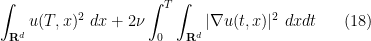
Now we work on verifying the energy inequality (18). Let ${\eta \in C^\infty_c({\bf R} \rightarrow {\bf R})}$ be a test function with ${\eta(0)=1}$ which is non-increasing on ${[0,+\infty)}$ . From (20) and integration by parts we have

$\displaystyle \int_0^\infty (-\eta'(t)) \int_{{\bf R}^d} |u^{(n)}(t,x)|^2\ dx dt + 2 \nu \int_0^\infty \eta(t) \int_{{\bf R}^d} |\nabla u^{(n)}(t,x)|^2\ dx dt = \int_{{\bf R}^d} |P_{\leq N_n} u_0(x)|^2\ dx.$

Taking limit inferior and using the Fatou-type lemma (2), we conclude that

$\displaystyle \int_0^\infty (-\eta'(t)) \int_{{\bf R}^d} |u(t,x)|^2\ dx dt + 2 \nu \int_0^\infty \eta(t) \int_{{\bf R}^d} |\nabla u(t,x)|^2\ dx dt$

$\displaystyle \leq \int_{{\bf R}^d} |u_0(x)|^2\ dx.$

Now let ${T>0}$ , take ${\eta = \eta_\varepsilon}$ to equal ${1}$ on ${[0,T]}$ and zero outside of ${[0,T+\varepsilon]}$ for some small ${\varepsilon}$ . Then we have

$\displaystyle \int_0^\infty (-\eta'_\varepsilon(t)) \int_{{\bf R}^d} |u(t,x)|^2\ dx dt + 2 \nu \int_0^T \int_{{\bf R}^d} |\nabla u(t,x)|^2\ dx dt$

$\displaystyle \leq \int_{{\bf R}^d} |u_0(x)|^2\ dx.$

The function ${-\eta'_\varepsilon}$ is supported on ${[T,T+\varepsilon]}$ , is non-negative, and has total mass one. By the Lebesgue differentiation theorem applied to the bounded measurable function ${t \mapsto \int_{{\bf R}^d} |u(t,x)|^2\ dx}$ , we conclude that for almost every ${T \in [0,+\infty)}$ , we have

$\displaystyle \int_0^\infty (-\eta'_\varepsilon(t)) \int_{{\bf R}^d} |u(t,x)|^2\ dx dt \rightarrow \int_{{\bf R}^d} |u(T,x)|^2\ dx$

as ${\varepsilon \rightarrow 0}$ . The claim (18) follows.

It remains to show that ${u}$ is a weak solution of (15), that is to say that (17) holds in the sense of spacetime distributions. Certainly the smooth solution ${u^{(n)}}$ of (19) will also be a weak solution, thus

$\displaystyle \partial_t u^{(n)}(t,x) + \partial_j P_{\leq N^{(n)}} \mathbb{P}( (P_{\leq N^{(n)}} u^{(n)}_j) (P_{\leq N^{(n)}} u^{(n)}) )(t,x) \ \ \ \ \ (22)$

$\displaystyle = \nu \Delta u^{(n)}(t,x) + P_{\leq N^{(n)}} u_0(x) \delta_0(t)$

in the sense of spacetime distributions on ${{\bf R} \times {\bf R}^d}$ , where we extend ${u^{(n)}}$ by zero outside of ${[0,+\infty) \times {\bf R}^d}$ .

At this point it is tempting to just take distributional limits of both sides of (22) to obtain (17). Certainly we have the expected convergence for the linear components of the equation:

$\displaystyle \partial_t u^{(n)} \rightharpoonup^* \partial_t u$

$\displaystyle \nu \Delta u^{(n)} \rightharpoonup^* \nu \Delta u$

$\displaystyle P_{\leq N^{(n)}} u_0(x) \delta_0(t) \rightharpoonup^* u_0(x) \delta_0(t).$

However, it is not immediately clear that

$\displaystyle \partial_j P_{\leq N^{(n)}} \mathbb{P}( (P_{\leq N^{(n)}} u^{(n)}_j) (P_{\leq N^{(n)}} u^{(n)}) ) \rightharpoonup^* \partial_j \mathbb{P}( u_j u ), \ \ \ \ \ (23)$

mainly because of the previously mentioned problem that multiplication is not continuous with respect to weak notions of convergence. But if we can show (23), then we do indeed recover (17) as the limit of (22), which will complete the proof of Theorem 14.

Let’s try to simplify the task of proving (23). The partial derivative operator ${\partial_j}$ is continuous with respect to convergence in distributions, so it suffices to show that

$\displaystyle P_{\leq N^{(n)}} F^{(n)}_j \rightharpoonup^* \mathbb{P}( u_j u ),$

where

$\displaystyle F^{(n)}_j := \mathbb{P}( (P_{\leq N^{(n)}} u^{(n)}_j) (P_{\leq N^{(n)}} u^{(n)}) ).$

We now try to get rid of the outer Littlewood-Paley projection. We claim that

$\displaystyle (1 - P_{\leq N^{(n)}}) F^{(n)}_j \rightharpoonup^* 0. \ \ \ \ \ (24)$

Let ${T>0}$ be a fixed time. By Sobolev embedding and (21), ${u^{(n)}}$ is bounded in ${L^2_t L^p_x([0,T] \times {\bf R}^d \rightarrow {\bf R}^d)}$ , uniformly in ${n}$ , for some ${2 < p < \infty}$ . The same is then true for ${P_{\leq N^{(n)}} u^{(n)}}$ , hence by Hölder’s inequality and Proposition 13, ${F^{(n)}}$ is uniformly bounded in ${L^1_t L^{p/2}_x([0,T] \times {\bf R}^d \rightarrow {\bf R}^d)}$ . On the other hand, for any spacetime test function ${\psi \in C^\infty_c({\bf R} \times {\bf R}^d)}$ , it is not difficult (using the rapid decrease of the Fourier transform of ${\psi}$ ) to show that ${(1 - P_{\leq N^{(n)}}) \psi}$ goes to zero in the dual space ${L^\infty_t L^{(p/2)'}_x([0,T] \times {\bf R}^d \rightarrow {\bf R})}$ . This gives (24).

It thus suffices to show that ${F^{(n)}_j}$ converges in the sense of distributions to ${\mathbb{P}( u_j u )}$ , thus one wants

$\displaystyle \int_{{\bf R} \times {\bf R}^d} (P_{\leq N^{(n)}} u^{(n)}_j) (P_{\leq N^{(n)}} u^{(n)}) \mathbb{P} \phi\ dx dt \rightarrow \int_{{\bf R} \times {\bf R}^d} u_j u \mathbb{P} \phi\ dx dt$

for any spacetime test function ${\phi}$ . One can easily calculate that ${\mathbb{P} \phi}$ lies in the dual space ${L^\infty_t L^{(p/2)'}_x([0,T] \times {\bf R}^d \rightarrow {\bf R})}$ to the space ${L^1_t L^{p/2}_x([0,T] \times {\bf R}^d \rightarrow {\bf R}^d)}$ that ${(P_{\leq N^{(n)}} u^{(n)}_j) (P_{\leq N^{(n)}} u^{(n)})}$ and ${u_j u}$ are bounded in, so it will suffices to show that ${P_{\leq N^{(n)}} u^{(n)}}$ converges strongly in ${L^2_t L^p_x(K \rightarrow {\bf R}^d)}$ to ${u}$ for ${p>2}$ sufficiently close to ${2}$ . and any compact subset ${K}$ of spacetime (since the ${L^\infty_t L^{(p/2)'}_x}$ norm of ${\mathbb{P} \phi}$ outside of ${K}$ can be made arbitrarily small by making ${K}$ large enough.)

Let ${N}$ be a dyadic integer, then we can split

$\displaystyle P_{\leq N^{(n)}} u^{(n)} - u = P_{\leq N}( u^{(n)}-u) + (P_{\leq N^{(n)}}-P_{\leq N}) u^{(n)} - (1-P_{\leq N}) u.$

The functions ${u^{(n)}, u}$ are uniformly bounded in ${L^2_t H^1_x([0,T] \times {\bf R}^d \rightarrow {\bf R}^d)}$ by some bound ${A}$ , hence by Plancherel’s theorem the functions ${(P_{\leq N^{(n)}}-P_{\leq N}) u^{(n)}}$ , ${(1-P_{\leq N}) u}$ have an ${L^2_t L^2_x([0,T] \times {\bf R}^d \rightarrow {\bf R}^d)}$ norm of ${O(A N^{-1})}$ (assuming ${n}$ is large enough so that ${N^{(n)} > N}$ ). Indeed, by Littlewood-Paley decomposition and Bernstein’s inequality we also see that these functions have an ${L^2_t L^p_x([0,T] \times {\bf R}^d \rightarrow {\bf R}^d)}$ norm of ${O( A N^{-1 + \frac{d}{2}-\frac{d}{p}})}$ if ${p>2}$ is close enough to ${2}$ that the exponent of ${N}$ is negative. It will therefore suffice to show that

$\displaystyle P_{\leq N}( u^{(n)} - u ) \rightarrow 0$

strongly in ${L^2_t L^p_x(K \rightarrow {\bf R}^d)}$ for every fixed ${N}$ and ${K}$ .

We already know that ${u^{(n)}-u}$ goes to zero in the sense of distributions, so (as Proposition 3 indicates) the main difficulty is to obtain compactness of the sequence. The ${P_{\leq N}}$ operator localises in spatial frequency, and the restriction to ${K}$ localises in both space and time, however there is still the possibility of escaping to temporal frequency. To prevent this, we need some sort of equicontinuity in time. For this, we may turn to the equation (19) obeyed by ${u^{(n)}}$ . Applying ${P_{\leq N}}$ , we see that

$\displaystyle \partial_t P_{\leq N} u^{(n)} + \partial_j P_{\leq N} F^{(n)}_j = \nu \Delta P_{\leq N} u^{(n)}$

when ${n}$ is large enough. Since ${P_{\leq N} u^{(n)}}$ is uniformly bounded in ${L^\infty_t L^2_x}$ and ${L^2_{t,loc} L^p_x}$ , we see from Hölder (and Proposition 13 that ${F^{(n)}_j}$ is bounded in ${L^\infty_t L^{q}_x([0,T] \times {\bf R}^d \rightarrow {\bf R}^d)}$ uniformly in ${n}$ for some ${q>1}$ , so by the Bernstein inequality ${\partial_j P_{\leq N} F^{(n)}_j}$ is bounded in ${L^2_t L^{\infty}_x([0,T] \times {\bf R}^d \rightarrow {\bf R}^d)}$ (we allow the bound to depend on ${N}$ ). Similarly for ${\nu \Delta P_{\leq N} u^{(n)}}$ . We conclude that ${\partial_t P_{\leq N} u^{(n)}}$ is bounded in ${L^2_t L^{\infty}_x([0,T] \times {\bf R}^d \rightarrow {\bf R}^d)}$ uniformly in ${n}$ ; taking weak limits using (2), the same is true for ${u}$ , and hence ${\partial_t P_{\leq N}( u^{(n)} - u )}$ is bounded in ${L^2_t L^{\infty}_x([0,T] \times {\bf R}^d \rightarrow {\bf R}^d)}$ . By the fundamental theorem of calculus and Cauchy-Schwarz, this gives Hölder continuity in time (of order ${1/2}$ ). Also, ${\nabla P_{\leq N}( u^{(n)} - u)}$ is bounded in ${L^\infty_t L^{\infty}_x([0,T] \times {\bf R}^d \rightarrow {\bf R}^d)}$ by Bernstein’s inequality; thus ${P_{\leq N}( u^{(n)} - u )}$ is equicontinuous in ${K}$ . By the Arzelá-Ascoli theorem and Proposition 3, ${P_{\leq N}(u^{(n)} - u)}$ must therefore go to zero uniformly on ${K}$ , and the claim follows. This completes the proof of Theorem 14.

Exercise 15 (Rellich compactness theorem) Let ${2 \leq p < \infty}$ be such that ${\frac{1}{p} > \frac{1}{2} - \frac{1}{d}}$ .

(i) Show that if ${u_n}$ is a bounded sequence in ${H^1({\bf R}^d \rightarrow {\bf R})}$ that converges in the sense of distributions to a limit ${u}$ , then there is a subsequence ${u_{n_j}}$ which converges strongly in ${L^p_{loc}({\bf R}^d \rightarrow {\bf R})}$ to ${u}$ (thus, for any compact set ${K \subset {\bf R}^d}$ , the restrictions of ${u_{n_j}}$ to ${K}$ converge strongly in ${L^p(K \rightarrow {\bf R})}$ to the restriction of ${u}$ to ${K}$ ).
(ii) Show that for any compact set ${K \subset {\bf R}^d}$ , the linear map ${\iota_K: H^1({\bf R}^d \rightarrow {\bf R}) \rightarrow L^p(K \rightarrow {\bf R})}$ defined by setting ${\iota_K u: K \rightarrow {\bf R}}$ to be the restriction of ${u: {\bf R}^d \rightarrow {\bf R}}$ to ${K}$ is a compact linear map.
(iii) Show that the above two claims fail at the endpoint ${\frac{1}{p} = \frac{1}{2} - \frac{1}{d}}$ (which of course only occurs when ${d>3}$ ).

The weak solutions constructed by Theorem 14 have additional properties beyond the ones listed in the above theorem. For instance:

Exercise 16 Let ${u_0}$ be as in Theorem 14, and let ${u}$ be a weak solution constructed using the proof of Theorem 14.

(i) Show that ${u}$ is divergence-free in the sense of spacetime distributions.
(ii) (Note: this exercise is tricky.) Assume ${d=3}$ . Show that the weak solution ${u}$ obeys a local energy inequality
$\displaystyle \int_{|x| \geq 2R} |u(T,x)|^2\ dx \leq \int_{|x| \geq R} |u_0(x)|^2 + O_{T,u_0}( \frac{1}{R} )$
for all ${T, R > 0}$ . (Hint: compute the time derivative of ${\int_{{\bf R}^3} |u^{(n)}(t,x)|^2 \psi(x/R)\ dx}$ , where ${\psi}$ is a smooth cutoff supported on ${B(0,2)}$ that equals one in ${B(0,1)}$ , and use Sobolev inequalities and Hölder to control the various terms that arise from integration by parts; one will need to expand out the Leray projection and use the fact that ${\partial_i \partial_j \Delta^{-1}}$ is bounded on every ${L^p({\bf R}^3)}$ space for ${1 < p < \infty}$ .) Using this inequality, show that there is a measure zero subset ${E}$ of ${[0,+\infty)}$ such that one has the energy inequality
$\displaystyle \int_{{\bf R}^d} u(T_2,x)^2\ dx + 2\nu \int_{T_1}^{T_2} \int_{{\bf R}^d} |\nabla u(t,x)|^2\ dx dt$

$\displaystyle \leq \int_{{\bf R}^d} u(T_1,x)^2\ dx$
for all ${T_1, T_2 \in [0,+\infty) \backslash E}$ with ${T_1 < T_2}$ . Furthermore, show that for all ${T \in [0,+\infty) \backslash E}$ , the time-shifted function ${u_T: [0,+\infty) \times {\bf R}^d \rightarrow {\bf R}^d}$ defined by ${u_T(t,x) := u(t+T, x)}$ is a weak solution to the initial value problem (15) with initial data ${u(T)}$ . (The arguments here can be extended to dimensions ${d \leq 4}$ , but it is open for ${d>4}$ whether one can construct Leray-Hopf solutions obeying the strong energy inequality.)
(iii) Show that after modifying ${u}$ on a set of measure zero, the function ${t \mapsto \int_{{\bf R}^d} u(t,x) \cdot v(x)\ dx}$ is continuous for any ${v \in L^2({\bf R}^d \rightarrow {\bf R}^d)}$ . (Hint: first establish this when ${v}$ is a test function.)

We will discuss some further properties of the Leray weak solutions in later notes.

— 4. Weak-strong uniqueness —

If ${u}$ is a (non-zero) element in a Hilbert space ${H}$ , and ${v}$ is another element obeying the inequality

$\displaystyle \|v\| \leq \|u\|, \ \ \ \ \ (25)$

then this is very far from the assertion that ${v}$ is equal to ${u}$ , since the ball ${\overline{B(0,\|u\|)}}$ of elements of ${H}$ obeying (25) is far larger than the single point ${\{u\}}$ . However, if one also posseses the information that ${v}$ agrees with ${u}$ when tested against ${u}$ , in the sense that

$\displaystyle \langle v,u \rangle = \langle u, u \rangle, \ \ \ \ \ (26)$

then (25) and (26) combine to indeed be able to conclude that ${u=v}$ . Geometrically, this is because the above-mentioned ball is tangent to the hyperplane described by (26) at the point ${u}$ . Algebraically, one can establish this claim by the cosine rule computation

$\displaystyle \| v-u\|^2 = \langle u,u \rangle - 2 \langle v,u \rangle + \langle v,v \rangle$

$\displaystyle = \langle v,v \rangle - \langle u, u \rangle$

$\displaystyle = \|v\|^2 - \|u\|^2$

$\displaystyle \leq 0$

giving the claim.

This basic argument has many variants. Here are two of them:

Exercise 17 (Weak convergence plus norm bound equals strong convergence (Hilbert spaces)) Let ${u}$ be an element of a Hilbert space ${H}$ , and let ${u_n}$ be a sequence in ${H}$ which weakly converges to ${u}$ , that is to say that ${\langle u_n, w \rangle \rightarrow \langle u, w \rangle}$ for all ${w \in H}$ . Show that the following are equivalent:

(i) ${\limsup_{n \rightarrow \infty} \|u_n \| \leq \|u\|}$ .
(ii) ${\lim_{n \rightarrow \infty} \|u_n \| = \|u\|}$ .
(iii) ${u_n}$ converges strongly to ${u}$ .

Exercise 18 (Weak convergence plus norm bound equals strong convergence ( ${L^1}$ norms)) Let ${(X,\mu)}$ be a measure space, let ${f: X \rightarrow [0,+\infty)}$ be an absolutely integrable non-negative function, and let ${f_n: X \rightarrow [0,+\infty)}$ be a sequence of absolutely integrable non-negative functions that converge pointwise to ${f}$ . Show that the following are equivalent:

(i) ${\limsup_{n \rightarrow \infty} \int_X f_n\ d\mu \leq \int_X f\ d\mu}$ .
(ii) ${\lim_{n \rightarrow \infty} \int_X f_n\ d\mu = \int_X f\ d\mu}$ .
(iii) ${f_n}$ converges strongly in ${L^1(X,\mu)}$ to ${f}$ .
(Hint: express ${\int_X |f_n-f|\ d\mu}$ and ${\int_X f_n-f\ d\mu}$ in terms of the positive and negative parts of ${f_n-f}$ . The latter can be controlled using the dominated convergence theorem.)

Exercise 19 Let ${u_0}$ be as in Theorem 14, and let ${u}$ be a weak solution constructed using the proof of Theorem 14. Show that (after modifying ${u}$ on a set of measure zero if necessary), ${u(t)}$ converges strongly in ${L^2({\bf R}^d \rightarrow {\bf R}^d)}$ to ${u_0}$ as ${t \rightarrow 0^+}$ . (Hint: use Exercise 16(iii) and Exercise 17.)

Now we give a variant relating to weak and strong solutions of the Navier-Stokes equations.

Proposition 20 (Weak-strong uniqueness) Let ${u: [0,T_*) \times {\bf R}^d \rightarrow {\bf R}^d}$ be an ${H^s}$ mild solution to the Navier-Stokes equations (15) for some ${u_0 \in H^s({\bf R}^d \rightarrow {\bf R}^d)}$ , ${0 < T_* \leq +\infty}$ , and ${s > \frac{d}{2}-1}$ with ${s \geq 1}$ . Let ${v: [0,T_*) \times {\bf R}^d \rightarrow {\bf R}^d}$ be a weak solution to the Navier-Stokes equation with ${v \in L^\infty_t L^2_x}$ and ${\nabla v \in L^2_t L^2_x}$ which obeys the energy inequality (18) for almost all ${0 \leq T < T_*}$ . Then ${u}$ and ${v}$ agree almost everywhere on ${[0,T_*) \times {\bf R}^d}$ .

Roughly speaking, this proposition asserts that weak solutions obeying the energy inequality stay unique as long as a strong solution exists (in particular, it is unique whenever it is regular enough to be a strong solution). However, once a strong solution reaches the end of its maximal Cauchy development, there is no further guarantee of uniqueness for the rest of the weak solution. Also, there is no guarantee of uniqueness of weak solutions if the energy inequality is dropped, and indeed there is now increasing evidence that uniqueness is simply false in this case; see for instance this paper of Buckmaster and Vicol for recent work in this direction. The conditions on ${u}$ can be relaxed somewhat (in particular, it is possible to drop the condition ${s \geq 1}$ ), though they still need to be “subcritical” or “critical” in nature; see for instance the classic papers of Prodi, of Serrin, and of Ladyzhenskaya, which show that weak solutions on ${[0,+\infty) \times {\bf R}^3}$ obeying the energy inequality are necessarily unique and smooth (after time ${t=0}$ ) if they lie in the space ${L^p_t L^q_r([0,+\infty) \times {\bf R}^3 \rightarrow {\bf R}^3)}$ for some exponents ${p,q}$ with ${\frac{2}{p} + \frac{3}{q} = 1}$ and ${2 \leq p < \infty}$ ; the endpoint case ${p=\infty}$ was worked out more recently by Escauriaza, Seregin, and Sverak. For a recent survey of weak-strong uniqueness results for fluid equations, see this paper of Wiedemann.

Proof: Before we give the formal proof, let us first give a non-rigorous proof in which we pretend that the weak solution ${v}$ can be manipulated like a strong solution. Then we have

$\displaystyle \partial_t v + \partial_j \mathbb{P}( v_j v ) = \nu \Delta v; \quad v(0) = u_0$

and

$\displaystyle \partial_t u + \partial_j \mathbb{P}( u_j u ) = \nu \Delta u; \quad u(0) = u_0.$

As in the beginning of the section, the idea is to analyse the ${L^2}$ norm of the difference ${w := v-u}$ . Writing ${v=u+w}$ in the first equation and subtracting from the second equation, we obtain the difference equation

$\displaystyle \partial_t w + \partial_j \mathbb{P}( w_j u + u_j w + w_j w ) = \nu \Delta w; \quad w(0) = 0.$

If we formally differentiate the energy ${E(t) := \frac{1}{2} \int_{{\bf R}^d} |w(t,x)|^2\ dx}$ using this equation, we obtain

$\displaystyle \partial_t E(t) = \int_{{\bf R}^d} - w \cdot \partial_j \mathbb{P}( w_j u + u_j w + w_j w ) + \nu w \cdot \Delta w\ dx$

(omitting the explicit dependence of the integrand on ${t}$ and ${x}$ ) which after some integration by parts (noting that ${\partial_j w}$ is divergence-free and thus is the identity on ${\mathbb{P}}$ ) formally becomes

$\displaystyle \partial_t E(t) = \int_{{\bf R}^d} \partial_j w \cdot ( w_j u + u_j w + w_j w ) - \nu |\nabla w|^2.$

The ${\partial_j w \cdot(u_j w)}$ and ${\partial_j w \cdot(w_j w)}$ terms formally cancel out by the usual trick of writing ${\partial_j w \cdot w}$ as a total derivative ${\frac{1}{2} \partial_j |w|^2}$ and integrating by parts, using the divergence-free nature ${\partial_j u_j= \partial_j w_j = 0}$ of both ${u}$ and ${w}$ . For the term ${\partial_j w \cdot(w_j u)}$ , we can cancel it against the ${\nu |\nabla w|^2}$ term by the arithmetic mean-geometric mean inequality

$\displaystyle \partial_j w \cdot(w_j u) \leq \nu |\nabla w|^2 + \frac{1}{4\nu} |w|^2 |u|^2$

to obtain

$\displaystyle \partial_t E(t) \leq \frac{1}{4\nu} \int_{{\bf R}^d} |w|^2 |u|^2 \leq \frac{1}{2\nu} E(t) \|u(t) \|_{L^\infty_x({\bf R}^d \rightarrow {\bf R}^d)}^2$

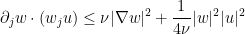
thanks to Hölder’s inequality. As ${u}$ is an ${H^s}$ mild solution, it lies in ${L^2_{t,loc} H^{s+1}_x}$ , which by Sobolev embedding and Hölder means that it is also in ${L^2_{t,loc} L^\infty_x}$ . Since ${E(0)=0}$ , Gronwall’s inequality then should give ${E(t)=0}$ for all ${t \geq 0}$ , giving the claim.

Now we begin the rigorous proof, in which ${v}$ is only known to be a weak solution. Here, we do not directly manipulate the difference equation, but instead carefully use the equations for ${u}$ and ${v}$ as a substitute. Define ${w}$ and ${E(t)}$ as before. From the cosine rule we have

$\displaystyle E(T) = \frac{1}{2} \int_{{\bf R}^d} |u(T)|^2\ dx + \frac{1}{2} \int_{{\bf R}^d} |v(T)|^2\ dx - \int_{{\bf R}^d} u(T) \cdot v(T)\ dx,$

where we drop the explicit dependence on ${x}$ in the integrand. From the energy inequality hypothesis (18), we have

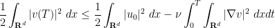$\displaystyle \frac{1}{2} \int_{{\bf R}^d} |v(T)|^2\ dx \leq \frac{1}{2} \int_{{\bf R}^d} |u_0|^2\ dx - \nu \int_0^T \int_{{\bf R}^d} |\nabla v|^2\ dx dt$

for almost all ${T}$ , where we also drop explicit dependence on ${t}$ in the integrand. The strong solution ${u}$ also obeys the energy inequality; in fact we have the energy equality

$\displaystyle \frac{1}{2} \int_{{\bf R}^d} |u(T)|^2\ dx = \frac{1}{2} \int_{{\bf R}^d} |u_0|^2\ dx - \nu \int_0^T \int_{{\bf R}^d} |\nabla u|^2\ dx dt$

as can be seen by first working with smooth solutions and taking limits using the local well-posedness theory. We conclude that

$\displaystyle E(T) \leq \int_{{\bf R}^d} |u_0|^2\ dx - \nu \int_0^T \int_{{\bf R}^d} |\nabla u|^2 + |\nabla v|^2\ dx dt - \int_{{\bf R}^d} u(T) \cdot v(T)\ dx \ \ \ \ \ (27)$

for almost all ${T}$ .

Now we work on the integral ${\int_{{\bf R}^d} u(T) \cdot v(T)\ dx}$ . Because we only know ${v}$ to solve the equation

$\displaystyle \partial_t v(t,x) + \partial_j \mathbb{P}( v_j v )(t,x) = \nu \Delta v(t,x) + u_0(x) \delta_0(t)$

in the sense of spacetime distributions, it is difficult to directly treat this spatial integral. Instead (similarly to the proof of the energy inequality for Leray solutions), we will first work with a proxy

$\displaystyle \int_{\bf R} \int_{{\bf R}^d} -\eta'(t) u \cdot v\ dx dt \ \ \ \ \ (28)$

where ${\eta \in C^\infty_c({\bf R} \rightarrow {\bf R})}$ is a test function in time, which we normalise with ${\eta(0)=1}$ ; eventually we will make ${\eta}$ an approximation to the indicator function of ${[-T,T]}$ and apply the Lebesgue differentiation theorem to recover information about ${\int_{{\bf R}^d} u(T) \cdot v(T)\ dx}$ for almost every ${T}$ .

By hypothesis, we have

$\displaystyle \int_{\bf R} \int_{{\bf R}^d} - v \cdot \partial_t \psi + \partial_j (v_j v) \cdot \mathbb{P} \psi + \nu \partial_j v \cdot \partial_j \psi\ dx dt = \int_{{\bf R}^d} u_0 \cdot \psi(0)\ dx$

for any spacetime test function ${\psi \in C^\infty_c({\bf R} \times {\bf R}^d \rightarrow {\bf R}^d)}$ . We would like to apply this identity with ${\psi}$ replaced by ${\eta(t) u}$ (in order to obtain an identity involving the expression (28)). Now ${\eta(t) u}$ is not a test function; however, as ${u}$ is an ${H^s}$ mild solution, it has the regularity

$\displaystyle \eta(t) u \in C^0_t H^s_x({\bf R} \times {\bf R}^d \rightarrow {\bf R}^d) \cap L^2_t H^{s+1}_x({\bf R} \times {\bf R}^d \rightarrow {\bf R}^d);$

also, using the equation (15), Sobolev embedding, Hölder’s inequality, and the hypotheses ${s > \frac{d}{2}-1}$ and ${s \geq 1}$ we see that

$\displaystyle \partial_t (\eta(t) u) \in L^2_t H^{-1}_x({\bf R} \times {\bf R}^d \rightarrow {\bf R}^d).$

(If one wishes, one can first obtain this bound for smooth solutions, and take limits using the local well-posedness theory.) As a consequence, one can find (for instance by using a combination of Littlewood-Paley projections and spatial cutoffs) a sequence of test functions ${\psi_n}$ , such that ${\psi_n}$ converges to ${\eta(t) u}$ in ${C^0_t H^s_x}$ and ${L^2_t H^{s+1}_x}$ norm (so ${\partial_j \psi_n}$ converges to ${\partial_j (\eta(t) u)}$ in ${L^2_t H^s_x}$ norm), and ${\partial_t \psi_n}$ converges to ${\partial_t (\eta(t) u)}$ in ${L^2_t H^{-1}_x}$ norm. Since ${v}$ lies in ${L^2_t H^1_x}$ , ${\partial_j v}$ lies in ${L^2_t L^2_x}$ , and ${\partial_j (v_j v)}$ lies in ${L^2_t L^1_x}$ by Hölder and Sobolev, we can take limits and conclude that

$\displaystyle \int_{\bf R} \int_{{\bf R}^d} - v \cdot \partial_t (\eta(t) u)+ \partial_j (v_j v) \cdot \mathbb{P} (\eta(t) u) + \nu \partial_j v \cdot \partial_j (\eta(t) u)\ dx dt$

$\displaystyle = \int_{{\bf R}^d} |u_0|^2\ dx.$

Since ${u}$ is divergence-free, and ${\eta(t)}$ does not depend on the spatial variables, we can simplify this slightly as

$\displaystyle \int_{\bf R} \int_{{\bf R}^d} - \eta'(t) u \cdot v - \eta(t) v \cdot \partial_t u + \eta(t) \partial_j (v_j v) \cdot u + \eta(t) \nu \partial_j v \cdot \partial_j u\ dx dt$

$\displaystyle = \int_{{\bf R}^d} |u_0|^2\ dx$

and so we can write (28) as

$\displaystyle \int_{\bf R} \eta(t) \int_{{\bf R}^d} [v \cdot \partial_t u - \partial_j (v_j v) \cdot u - \nu \partial_j v \cdot \partial_j u]\ dx dt$

$\displaystyle + \int_{{\bf R}^d} |u_0|^2\ dx.$

Using the Lebesgue differentiation theorem as in the proof of Theorem 14, we conclude that for almost every ${T}$ , one has the identity

$\displaystyle \int_{{\bf R}^d} u(T) \cdot v(T)\ dx = \int_0^T \int_{{\bf R}^d} [v \cdot \partial_t u - \partial_j (v_j v) \cdot u - \nu \partial_j v \cdot \partial_j u]\ dx dt$

$\displaystyle + \int_{{\bf R}^d} |u_0|^2\ dx.$

Applying (15), the right-hand side is

$\displaystyle \int_0^T \int_{{\bf R}^d} -v \cdot \mathbb{P} \partial_j(u_j u) - \partial_j (v_j v) \cdot u + \nu v \cdot \Delta u - \nu \partial_j v \cdot \partial_j u\ dx dt + \int_{{\bf R}^d} |u_0|^2\ dx.$

(Note that expressions such as ${\int_0^T \int_{{\bf R}^d} v \cdot \Delta u\ dx dt}$ are well defined because ${u, v}$ lie in ${L^2_t H^1_x([0,T] \times {\bf R}^d \rightarrow {\bf R}^d)}$ .) We can integrate by parts (justified using the usual limiting argument and the bounds on ${u,v}$ ) and use the divergence-free nature of ${v}$ to write this as

$\displaystyle \int_0^T \int_{{\bf R}^d} -v \cdot \partial_j(u_j u) - u \cdot \partial_j (v_j v) - 2\nu \partial_j v \cdot \partial_j u\ dx dt + \int_{{\bf R}^d} |u_0|^2\ dx.$

Inserting this into (27), we conclude that

$\displaystyle E(T) \leq \int_0^T \int_{{\bf R}^d} - u \cdot \partial_j (v_j v) - v \cdot \partial_j(u_j u) - \nu |\nabla v - \nabla u|^2\ dx dt.$

We write ${v = u + w}$ and write this as

$\displaystyle E(T) \leq \int_0^T \int_{{\bf R}^d} - u \cdot \partial_j (2 u_j u + w_j u + w u_j + w_j w) - w \cdot \partial_j(u_j u)$

$\displaystyle - \nu |\nabla w|^2\ dx dt,$

noting from the regularity ${w \in C^0_t L^2_x \cap L^2_t H^1_x}$ , ${u \in C^0_t H^s_x \cap L^2_t H^{s+1}_x}$ on ${[0,T] \times {\bf R}^d}$ and Sobolev embedding that one can ensure that all integrals here are absolutely convergent.

The integral ${\int_0^T \int_{{\bf R}^d} u \cdot \partial_j (2 u_j u)\ dx dt}$ can be rewritten using integration by parts as ${-2\int_0^T \int_{{\bf R}^d} u_j (\partial_j u) \cdot u\ dx dt}$ (noting that there is enough regularity to justify the integration by parts by the usual limiting argument); expressing ${\partial_j u \cdot u}$ as a total derivative ${\frac{1}{2} \partial_j |u|^2}$ and integrating by parts again using the divergence-free nature of ${u}$ , we see that this expression vanishes. Similarly for the ${u \cdot \partial_j (w_j u)}$ term. Now we eliminate the remaining terms which are linear in ${w}$ :

$\displaystyle \int_0^T \int_{{\bf R}^d} -u \cdot \partial_j (w u_j) - w \cdot \partial_j(u_j u).$

We may integrate by parts, and write the dot product in coordinates, to write this as

$\displaystyle \int_0^T \int_{{\bf R}^d} (\partial_j u_k) w_k u_j - w_k \cdot \partial_j(u_j u_k).$

Applying the Leibniz rule and the divergence-free nature of ${u}$ , we see that this expression vanishes. We conclude that

$\displaystyle E(T) \leq \int_0^T \int_{{\bf R}^d} - u \cdot \partial_j (w_j w) - \nu |\nabla w|^2\ dx dt.$

Now we use the Leibniz rule, the divergence-free nature of ${w}$ , and the arithmetic mean-geometric mean inequality to write

$\displaystyle |u \cdot \partial_j(w_j w)| \leq |u| |w| |\nabla w| \leq \nu |\nabla w|^2 + \frac{1}{4 \nu} |u|^2 |w|^2$

to obtain

$\displaystyle E(T) \leq \frac{1}{4\nu} \int_0^T \int_{{\bf R}^d} |u|^2 |w|^2$

and hence by Sobolev embedding we have

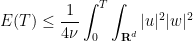
$\displaystyle E(T) \lesssim_{d,s,\nu} \| u \|_{L^2_t H^{s+1}_x([0,T] \times {\bf R}^d)} \int_0^T E(t)\ dt$

for almost all ${T \in [0,T_*)}$ . Applying Gronwall’s inequality (modifying ${E}$ on a set of measure zero) we conclude that ${E(T) = 0}$ for almost all ${T}$ , giving the claim. $\Box$

One application of weak-strong uniqueness results is to give (in the ${d=3}$ case at least) partial regularity on the weak solutions constructed by Leray, in that the solutions ${u}$ agree with smooth solutions on large regions of spacetime – large enough, in fact, to cover all but a measure zero set of times ${t}$ . Unfortunately, the complement of this measure zero set could be disconnected, and so one could have different smooth solutions agreeing with ${u}$ at different epochs, so this is still quite far from an assertion of global regularity of the solution. Nevertheless it is still a non-trivial and interesting result:

Theorem 21 (Partial regularity) Let ${d=3}$ . Let ${u_0}$ be as in Theorem 14, and let ${u}$ be a weak solution constructed using the proof of Theorem 14.

(i) (Eventual regularity) There exists a time ${0 < T_0 < +\infty}$ such that (after modification on a set of measure zero), the weak solution ${u}$ on ${[T_0,+\infty) \times {\bf R}^3}$ agrees with an ${H^1}$ mild solution on ${[T_0,+\infty) \times {\bf R}^3}$ with initial data ${u(T_0) \in H^1_x({\bf R}^3 \rightarrow {\bf R}^3)}$ (where we time shift the notion of a mild solution to start at ${T_0}$ instead of ${0}$ ).
(ii) (Epochs of regularity) There exists a compact exceptional set ${E \subset [0,+\infty)}$ of measure zero, such that for any time ${t \in [0,+\infty) \backslash E}$ , there is a time interval ${[T_1,T_2]}$ containing ${t}$ in its interior such that ${u}$ on ${[T_1,T_2] \times {\bf R}^3}$ agrees almost everywhere whtn an ${H^1}$ mild solution on ${[T_1,T_2] \times {\bf R}^3}$ with initial data ${u(T_1) \in H^1_x({\bf R}^3 \rightarrow {\bf R}^3)}$ .

Proof: (Sketch) We begin with (i). From (18), the ${L^2_t L^2_x([0,+\infty) \times {\bf R}^3 \rightarrow {\bf R}^3)}$ norm of ${\nabla u}$ and the ${L^\infty_t L^2_x([0,+\infty) \times {\bf R}^3 \rightarrow {\bf R}^3)}$ norm of ${u}$ are finite. Thus, for any ${\varepsilon>0}$ , one can find a positive measure set of times ${T}$ such that

$\displaystyle \| \nabla u(T) \|_{L^2_x({\bf R}^3 \rightarrow {\bf R}^9)} \| u(T) \|_{L^2_x({\bf R}^3 \rightarrow {\bf R}^3)} \leq \varepsilon$

which by Plancherel and Cauchy-Schwarz implies that

$\displaystyle \| u(T) \|_{\dot H^{1/2}_x({\bf R}^3 \rightarrow {\bf R}^3)} \lesssim \varepsilon^{1/2}.$

In particular, by Exercise 16, one can find a time ${T_0}$ such that ${u}$ is a weak solution on ${[T_0,+\infty)}$ with initial data ${u(T_0) \in H^1_x({\bf R}^3 \rightarrow {\bf R}^3)}$ obeying the energy inequality, with

$\displaystyle \| u(T_0) \|_{\dot H^{1/2}_x({\bf R}^3 \rightarrow {\bf R}^3)} \lesssim \varepsilon^{1/2}.$

By the small data global existence theory (Theorem 45 from Notes 1), if ${\varepsilon>0}$ is chosen small enough, then there is then a global ${H^1}$ mild solution on ${[T_0,+\infty) \times {\bf R}^3}$ to the Navier-Stokes equations with initial data ${u(T_0)}$ , which must then agree with ${u}$ by weak-strong uniqueness. This proves (i).

Now we look at (ii). In view of (i) we can work in a fixed compact interval ${[0,T_0]}$ . Let ${0 < t \leq T_0}$ be a time, and let ${\varepsilon>0}$ be a sufficiently small constant. If there is a positive measure set of times ${0 < T_1 < t}$ for which

$\displaystyle \| u(T_1) \|_{H^1_x({\bf R}^3)} \leq \varepsilon / (T_1-t)^{1/4},$

then by the same argument as above (but now using ${H^1}$ well-posedness theory instead of ${\dot H^{1/2}}$ well-posedness theory, which was not explicitly covered in previous notes but can be handled by variants of the techniques there), we will be able to equate ${u}$ (almost everywhere) with an ${H^1}$ mild solution on ${[T_1,T_2] \times {\bf R}^3}$ for some neighbourhood ${[T_1,T_2]}$ of ${t}$ . Thus the only times ${t}$ for which we cannot do this are those for which one has

$\displaystyle \| u(T_1) \|_{H^1_x({\bf R}^3)} \geq \varepsilon / (T_1-t)^{1/4}$

for almost all ${0 < T_1 < t}$ . In particular, using Vitali-type covering lemmas, for any ${\delta>0}$ , one can cover such times by the doubles of a finite collection of intervals of length ${\delta}$ , such that ${\| u(T)\|_{H^1_x({\bf R}^3)} \gtrsim \delta^{-1/4}}$ for almost every ${T}$ in that interval. On the other hand, as ${u}$ is bounded in ${L^2_t H^1_x([0,T_0] \times {\bf R}^3 \rightarrow {\bf R}^3)}$ , the number of disjoint time intervals of this form is at most ${O( \delta^{-1/2} )}$ (where we allow the implied constant to depend on ${u}$ and ${T_0}$ ). Thus the set of exceptional times can be covered by ${O(\delta^{-1/2})}$ intervals of length ${\delta}$ , and thus its closure has Lebesgue measure ${O(\delta^{1/2})}$ . Sending ${\delta \rightarrow 0}$ we see that the exceptional times are contained in a closed measure zero subset of ${[0,T_0]}$ , and the claim follows. $\Box$

The above argument in fact shows that the exceptional set ${E}$ in part (ii) of the above theorem will have upper Minkowski dimension at most ${1/2}$ (and hence also Hausdorff dimension at most ${1/2}$ ). There is a significant strengthening of this partial regularity result due to Caffarelli, Kohn, and Nirenberg, which we will discuss in later notes.

48 comments

Comments feed for this article

2 October, 2018 at 5:56 pm

Quanling Deng

Reblogged this on gonewithmath.

3 October, 2018 at 3:44 am

Gabriel Apolinario

These notes are a great resource.
Terry, there’s a missing word in the first paragraph: “are not high enough regularity”

[Reworded – T.]

3 October, 2018 at 6:16 am

Dr. Anil Pedgaonkar

Why maths people are left with old topics like fluid mechanics while topics like relativity theory string theory quantum theory are with physics

3 October, 2018 at 9:14 am

Anonymous

Turbulence is still not well understood and since we live in turbulent times it may become a contemporary subject.

4 October, 2018 at 10:53 pm

Anonymous

No doubt you are aware of https://en.wikipedia.org/wiki/Straw_man in your post, but let us overlook that. The reason why fluid mechanics, in particular Navier-Stokes equations, is mathematically interesting is that its behavior is not well-understood, even though its formulation is extremely simple. Anyone with modest math education can “understand” the governing equations, but no-one knows whether they are well-posed for arbitrarily long time intervals. Certainly there are open problems and plenty of theory building to be done in string theory and other fields practiced by “big bad physicists” where the problem setting itself is more complicated, but one is simply less surprised to encounter unsolved problems in more complicated settings. Moreover, all the fields you mentioned belong to mathematical physics and are under active research by quite a few well-trained people who consider themselves primarily as mathematicians.

4 October, 2018 at 11:26 pm

Juha-Matti Perkkiö

Prof. Tao,

the recent polymath-projects discussed in this blog have been very inspiring and seem to be rather efficient when their goals are set properly. Could there be a case for some kind of mixed analysis/numerical analysis/computational project to gain some insight on Navier-Stokes? What comes to mind is for example to generate solutions with H^2- or H^1-norm growing as fast as possible/decaying as slow as possible or perhaps to generate solutions decaying as fast as possible in some relevant weaker norm like L^2. I am aware that even the existence of suitable quantitative criteria for the reliability of such numerical experiments is not self-evident, but perhaps there are some.

5 October, 2018 at 12:44 pm

Sam

Apologies, I must be missing something basic, but why do the bounds on the $L^\infty_t L^2_x$ norm of $u^{(n)}$ and $L^2_tL^2_x$ -norm of $\nabla u^{(n)}$ imply an $L^\infty_t H^1$ bound on $u$ ?

5 October, 2018 at 12:45 pm

Sam

Sorry, I should specify that I’m talking about estimate (21).

5 October, 2018 at 2:23 pm

Terence Tao

This was a typo: it has been corrected to $L^2_t H^1_x$ .

7 October, 2018 at 1:55 am

Sam

Ah, yes, that makes sense. Thanks!

7 October, 2018 at 5:14 am

Huang

Terry，I am Chinese. I have a new opinion about Callatz Conjecture. How can I send it to you?

8 October, 2018 at 9:29 am

Anonymous

Are you Huang Deren mathematician?

8 October, 2018 at 4:18 pm

Huang

9 October, 2018 at 12:44 pm

254A, Notes 3: Local well-posedness for the Euler equations | What's new

[…] weak compactness (Proposition 2 of Notes 2), one can pass to a subsequence such that converge weakly to some limits , such that and all […]

8 November, 2018 at 5:48 am

Stefan

As a double major in theoretical physics/theoretical computer science, I’m very intersted in this.

Does anybody know if this is related to “Homotopy Analysis Method in Nonlinear Differential Equations” and “Liao’s Method of Directly Defining the Inverse Mapping (MDDiM).”?

https://www.researchgate.net/publication/266832165_Homotopy_Analysis_Method_in_Nonlinear_Differential_Equations

https://link.springer.com/article/10.1007/s11075-015-0077-4

Anyway, since reading the post about ultrafilters and hierarchical infinitesimals, I feel that more boundries between physics and computer science could be broken and new solutions be found.

I think it is about time to solve the crisis in physics

8 November, 2018 at 3:39 pm

Anonymous

In physics, the subjective(!) description “more beautiful” for a desired feature of a better new theory should be replaced (or interpreted) by the objective(!) description “more symmetrical”. It is interesting to observe that each new physical theory is indeed “more symmetrical” (i.e. invariant under a larger group of transformations) – leading to (the already observed) microscopic “fearfull symmetry” for all known elementary particles interactions, and also macroscopically for gravitation.

9 December, 2018 at 2:32 pm

254A, Supplemental: Weak solutions from the perspective of nonstandard analysis (optional) | What's new

[…] a Notes 2, we reviewed the classical construction of Leray of global weak solutions to the Navier-Stokes […]

16 December, 2018 at 2:37 pm

255B, Notes 1: The Lagrangian formulation of the Euler equations | What's new

[…] Despite the popularity of the initial condition (4), we will try to keep conceptually separate the Eulerian space from the Lagrangian space , as they play different physical roles in the interpretation of the fluid; for instance, while the Euclidean metric is an important feature of Eulerian space , it is not a geometrically natural structure to use in Lagrangian space . We have the following more general version of Exercise 8 from 254A Notes 2: […]

23 February, 2019 at 10:28 am

Guilherme Rezende

You have tried solutions in the form: $u_{i}(x,t)=u_{i}^{0}+\frac{c_{i}te^{-t}}{cosh(k_{1}x_{1}+k_{2}x_{2}+k_{3}x_{3})}$ with $c_{2}+c_{3}+c_{4}=0$ and $k_{1}c_{1}+k_{2}c_{2}+k_{3}c_{3}=0$ ? they work

2 April, 2019 at 6:42 pm

Zaher

In the discussion following (24), it is said that {u^{(n)}} is bounded in {L^\infty_t L^p_x}, uniformly in {n}, for some {2 < p < \infty}. But we only have uniform {L_2 H^1} control which would give {L_t^2 L_x^p}. As a consequence, {F_j^N} is uniformly bounded in {L_t^1 L_x^{p/2}}. This does not affect the argument, apart from some apparent typos.

[Corrected, thanks – T.]

13 April, 2019 at 4:23 am

Anonymous

If one considers the Dirichlet boundary conditions on a bounded domain, does the Leray projection preserve the boundary condition?

7 August, 2019 at 6:25 am

Martin

Hello, I am interested in the solutions of the Navier-Stokes equations.
Is a weak solution for the 3D Navier-Stokes equations locally unique?
If $u$ , $v$ are two weak Leray solutions for the 3D Navier-Stokes equations with
$u(0)=v(0)$ (1)
Then there is a small $\delta > 0$ ,
such that $u(t)=v(t)$ for all $t\in[0,\delta]$ (2).
Is it true that (1) implies (2) using weak continuity, energy inequality?

7 August, 2019 at 7:31 am

Terence Tao

I am not aware of such a result (and this would likely be of comparable difficulty as establishing global uniqueness for Leray-Hopf solutions, which is not universally believed to be true). It is true however that $u(t)-v(t)$ will converge strongly to zero in $L^2$ as $t \to 0$ (possibly after modifying the weak solution on a measure zero set of times), thanks to Exercise 19. And weak-strong uniqueness will kick in if one of the weak solutions $u,v$ is strong.

7 August, 2019 at 1:24 pm

Martin

We assume that the following assertion is true:
Let u, v two weak Leray solutions of the 3D Navier-Stokes equations on $[a,T]$ , with $a>0$ corresponding to the same data $u(a)$ .
Then $u(t)=v(t)$ almost everywhere on $[a,T]$ .
Is this an uniqueness result for weak Leray solutions of the 3D Navier-Stokes equations ?
Or, It must to extend this to $a=0$ .

8 August, 2019 at 7:08 am

Terence Tao

This would depend rather sensitively on how one actually defines the notion of a “weak Leray solution on $[a,T]$ “. For instance, would one require the energy inequality (18) to hold starting from time $t=a$ , or from time $t=0$ ? Similarly for the distributional initial value condition (17). With weak solutions one has to be very careful with the precise definitions and hypotheses, as it is very easy to make subtle errors in one’s reasoning otherwise by blindly applying a fact that is true for classical solutions to one or more weak solutions. For instance, depending on how precisely one defines a “Leray weak solution”, the time translation $(t,x) \mapsto u(t+a,x)$ of a Leray weak solution $u$ may not itself be a Leray weak solution, even though the corresponding fact for classical solutions is trivially true.

3 June, 2020 at 6:36 am

Antoine

At the end of the lecture, you said that you would cover the Caffarelli-Kohn-Nirenberg theorem, which I would like to read about. However, the later notes only cover Euler equations related topics. Do you stil plan on writing notes on this matter?

[No – T.]

17 October, 2020 at 3:59 pm

Anonymous

Before Exercise 4:

Thanks to the fundamental theorem of calculus for locally integrable functions, we still recover the unique solution (16):

and also in Exercise 4(ii):

One has (16) for almost all ${t \in [0,T)}$ .

“(16)” is linked to equation (3).

[Corrected, thanks – T.]

20 October, 2020 at 3:37 pm

Anonymous

At the level of set function, a function $u:[0,T]\times \mathbf{R}^d\to\mathbf{R}$ can be always interpreted as
$u:[0,T]\to X$ where $X$ is the set of functions from $\mathbf{R}^d$ to $\mathbf{R}$ and $(u(t))(x)=u(t,x)$ .

If one puts extra assumptions on $u$ so that $u(t)\in X$ for all $t$ and $X$ is some nice (separable, self-reflexive, …) Banach space, then there are two ways to define the weak partial derivative $\partial_tu$ .

One way is to define it as a distribution on $\mathbf{R}\times\mathbf{R}^d$ , as in this set of notes, which is a continuous linear functional on $C_c^\infty(\mathbf{R}\times\mathbf{R}^d\to\mathbf{R})$ (with the smooth topology). This notion does not depend on the structure of $X$ mentioned above.

Another way is that if one knows in addition, $u\in L^1((0,T);X)$ , i.e., $u$ is strongly measurable such that $\int_{[0,T]}\|u(t)\|_{X}dt<\infty$ , one can define $u'=v\in L^1((0,T);X)$ be the "weak derivative of $u$ where
$\displaystyle \int_0^T\phi'(t)u(t)dt=-\int_0^T\phi(t)v(t)dt$
for all $\phi\in C_c^\infty((0,T)\to\mathbf{R})$ . Here $u'$ is a continuous functional on $C_c^\infty((0,T))$ .

Are these two notions of "weak derivative" somehow equivalent to each other so that one can always write one in terms of another and safely use them interchangeably?

21 October, 2020 at 11:09 am

Terence Tao

As a general rule, any two “good” notions of weak or strong derivative (or integral, or other standard linear operation) would be expected to coincide on their common domain of definition. One reason for this is that (i) almost all the usual domains of definition admit some nice class of test functions which are dense these domains in suitable topologies; (ii) a “good” interpretation of the operation in question tends to be weakly continuous with respect to these topologies (e.g., as measured in the distributional topology), and (iii) weak limits are unique. It would be a good exercise for you to work out this scheme for the two notions of derivative you describe here to show that they are compatible on the common domain of definition.

21 October, 2020 at 4:23 pm

Anonymous

… by the definition
$\displaystyle \langle \partial_i \lambda, \phi \rangle := - \langle \lambda, -\partial_i \phi \rangle$

There is a redundant negative sign.

… Two distributions ${\lambda, \eta}$ are equal in the sense of distributions of ${\langle \lambda, \phi \rangle = \langle \eta, \phi \rangle}$ for all ${\phi \in C^\infty(U \rightarrow {\bf R})}$ …

I think the subscript $c$ is missing in $C^\infty(U \rightarrow {\bf R})$ .

[Corrected, thanks – T.]

21 October, 2020 at 4:54 pm

Anonymous

Could you elaborate on how Exercise 4 is done by the fundamental theorem of calculus for locally integrable functions?

By definition, (i) is the same as

$\displaystyle -\int_0^Tu\partial_t\phi(s)\,ds = u_0\phi(0)+\int_0^Tf(s)\phi(s)\,ds\ \ \ \ \ \ (*)$

for every $\phi\in C_c^{\infty}((-\infty,T))$ . How does this lead to (3) almost everywhere?

On the other hand, if one assumes (3) almost everywhere, then (*) is true for some special test function $\phi$ . How does it generalize to every $\phi\in C_c^{\infty}((-\infty,T))$ ?

23 October, 2020 at 7:51 am

Terence Tao

For the first implication, it suffices by the second implication and linearity to verify the case $u_0=f=0$ . By the fundamental theorem of calculus, any function in $C^\infty_c((-\infty,T))$ is equal on $[0,T]$ to the derivative of another function on $C^\infty_c((-\infty,T))$ .

For the second implication, insert (3) into the left-hand side of (*), then apply Fubini’s theorem and then the fundamental theorem of calculus (the regularity hypotheses on $u,f,\phi$ are more than sufficient to justify the formal manipulations).

21 October, 2020 at 5:07 pm

Anonymous

In section 2, when defining the weak solution using (4), $u$ is required to be “locally integrable”. In the more general setting of (5), $u$ is said to be “locally bounded”. Are these two notions equivalent?

23 October, 2020 at 7:53 am

Terence Tao

No. For instance if $q_n$ is an enumeration of the rationals then $\sum_{n=1}^\infty 2^{n} 1_{[q_n,q_n+4^{-n}]}$ is locally integrable (in fact globally integrable) but not locally bounded. On the other hand all locally bounded functions are locally integrable.

22 October, 2020 at 9:42 am

Anonymous

In the proof of Theorem 14,

… This is enough regularity for Proposition 2 to apply, and we can pass to a subsequence of ${u^{(n)}}$ which converges in the sense of spacetime distributions in ${{\bf R} \times{\bf R}^d}$ (after extending by zero outside of ${[0,+\infty) \times {\bf R}^d \rightarrow {\bf R}^d}$ to a limit ${u}$ , which is in ${L^\infty_t H^1_x([0,T] \times {\bf R}^d \rightarrow {\bf R}^d)}$ for every ${T}$ .

(A piece of parenthesis is missing and I guess you mean extending by zero outside of $[0,+\infty) \times {\bf R}^d$ .)

[Typos corrected, also $L^\infty_t H^1_x$ should be $L^2_t H^1_x$ -T.]

I try to understand how Banach-Alaoglu (Prop 2) is used here. In particular, what is $\|\|_X$ and what is $\|\|_{X^*}$ in the argument above?

[Here $X^* = L^2_t H^1_x$ and $X$ is the predual space $L^2_t H^{-1}_x$ (or one can use the Riesz representation theorem for Hilbert spaces and take $X=X^*$ with the usual Riesz identification). -T.]

22 October, 2020 at 10:05 am

Anonymous

I’m confused with the topologies on the linear space $C_c^{\infty}(U\to\mathbf{R})$ .

In the definition of distributions on $U$ , there is a “standard” topology $\tau$ on $C_c^{\infty}(U\to\mathbf{R})$ that one defines the continuous linear functionals on $C_c^{\infty}(U\to\mathbf{R})$ as distributions on $U$ .

On the other hand, with a different norm/seminorm $\|\|_X$ on $C_c^{\infty}(U\to\mathbf{R})$ in the hypothesis of Proposition 2, one has different topology $\tau_X$ . How does $\tau_X$ compare to $\tau$ ? How does one know that element in $X^*$ is a “distribution” so that one can talk about “converges in the sense of distributions” in Proposition 2?

23 October, 2020 at 12:53 pm

Terence Tao

Virtually every function space norm one works with in analysis, when restricted to test functions, gives a topology that is weaker than the test function topology, hence every linear functional that is continuous with respect to the norm topology will also be continuous with respect to the test function topology, and is hence a distribution.

23 October, 2020 at 4:09 pm

Anonymous

(I tried to post the following comment previously. But I don’t know why it was classified as spam by WordPress…)

In the “approximate solutions” stage of the proof of Theorem 14, what is the purpose of introducing the notion of $H^s$ -mild solution to (15) on a time interval $[0,T]$ ?

It is said after the $H^s$ -mild solution definition that

… By a modification of the theory of the previous set of notes, we thus see that there is a maximal Cauchy development ${u^{(n)}: [0,T_*^{(n)}) \times {\bf R}^d \rightarrow {\bf R}^d}$ that is a *smooth* solution to (19) (and an ${H^s}$ -mild solution for every ${s \geq 0})$ , with ${\|u^{(n)} \|_{L^\infty_t L^\infty_x([0,T_*^{(n)}))} = \infty}$ if ${T_*^{(n)} < \infty}$ .

Isn’t being smooth better than being $H^s$ -mild?

Later,

… From (19) we know that ${u^{(n)}}$ and ${\partial_t u^{(n)}}$ lie in ${C^0_t H^s_x([0,T] \times {\bf R}^d \rightarrow {\bf R}^d)}$ for any ${s \geq 0}$ and any ${0 < T < T_*}$ .

why the *smooth* $u^{(n)}$ now only lie in ${C^0_t H^s_x([0,T] \times {\bf R}^d \rightarrow {\bf R}^d)}$ ?

23 October, 2020 at 7:38 pm

Terence Tao

Smoothness does not imply decay in space, so a smooth function does not automatically lie in $H^s_x$ .

24 October, 2020 at 6:29 am

Anonymous

In the last big step of the proof of Theorem 14, the problem is reduced to showing (23):

$\displaystyle \partial_j P_{\leq N^{(n)}} \mathbb{P}( (P_{\leq N^{(n)}} u^{(n)}_j) (P_{\leq N^{(n)}} u^{(n)}) ) \rightharpoonup^* \partial_j \mathbb{P}( u_j u ), \ \ \ \ \ (23)$

which, by several intermediate steps, is reduced to showing that
$\displaystyle P_{\leq N}( u^{(n)} - u ) \rightarrow 0$
strongly in ${L^2_t L^p_x(K \rightarrow {\bf R}^d)}$ for every fixed ${N}$ and ${K}$ .

If one wants to apply Proposition 3 (with some appropriate $X^*$ and $Y^*$ ) at some point, then it should be that $Y^*=L^2_t L^p_x(K \rightarrow {\bf R}^d)$ (right?). The sequence itself is not a space, what should $X^*$ be?

By showing that

${\partial_t P_{\leq N}( u^{(n)} - u )}$ is bounded in ${L^2_t L^{\infty}_x([0,T] \times {\bf R}^d \rightarrow {\bf R}^d)}$

and

${\nabla P_{\leq N}( u^{(n)} - u)}$ is bounded in ${L^\infty_t L^{\infty}_x([0,T] \times {\bf R}^d \rightarrow {\bf R}^d)}$

the later paragraph shows that ${P_{\leq N}( u^{(n)} - u )}$ is equicontinuous in ${K}$ . In order to apply Arzela-Ascoli theorem, a pointwise bound for ${P_{\leq N}( u^{(n)} - u )}$ is also needed (isn’t it?), is it alluded somewhere?

Also, when the Arzela-Ascoli theorem is applied, does one only have a uniformly convergent subsequence of ${P_{\leq N}( u^{(n)} - u )}$ instead of the sequence itself as stated in the penultimate sentence of the proof? Would you elaborate how Proposition 3 is used there?

25 October, 2020 at 4:08 pm

Terence Tao

Proposition 3 can applied with $\| u \|_{Y^*}$ being the sum of the $L^2_t L^\infty_x(K \times [0,T])$ norm of $\partial_t u$ , the $L^\infty_t L^\infty_x(K \times [0,T])$ norm of $\nabla u$ , and the $L^\infty_x(K)$ norm of $u(0)$ (to get the lower order term, which in this case vanishes for $n$ large enough), and $X^* = L^\infty_t L^\infty_x(K \times [0,T])$ , with the Arzela-Ascoli theorem giving the required compact embedding. (One can check that these spaces have appropriate preduals $X,Y$ ; one can also use the proof of Proposition 3 directly rather than using it as a black box to obtain a similar conclusion, for instance the Urysohn subsequence principle can be used to deal with the subsequence problem you mentioned.)

29 October, 2020 at 5:36 pm

Anonymous

In the definition (17) of the “weak solution” right before Theorem 14, is the divergence-free condition for $u$ hiding somewhere so that one does not need to incorporate it into the definition?

Does the mentioned definition (17) remain the same if one only considers the spacetime test functions that are (space) divergence-free?.

29 October, 2020 at 6:01 pm

Anonymous

1. If the data is div-free then solutions to this equation are always div-free.
2. The test function here is scalar-valued so this doesn’t make sense. If instead you dot it with a vector-valued test function, the answer is yes because of the Hodge decomposition.

30 October, 2020 at 8:24 am

Anonymous

In the case when $V$ is a finite-dimensional vector space, particularly in the definition of “weak solutions” after Exercise 4, the notion of “distributions” seems to be no longer a continuous linear functional on the space $C_c^\infty({\bf R}^n)$ but a map from $C_c^\infty({\bf R}^n)$ to $V$ .

On the other hand, one can consider the vector-valued test functions ${\boldsymbol \phi}\in [C_c^\infty((-\infty, T))^n]^n$ in the definition of weak solution:
$\displaystyle - \int_0^T u(s) \cdot\partial_t {\boldsymbol \phi}(s)\ ds = u_0 \cdot{\boldsymbol \phi}(0) + \int_0^T F(u(s))\cdot {\boldsymbol \phi}(s)\ ds$
where $V$ is endowed with an inner product structure. In this case, one has linear functionals on $[C_c^\infty((-\infty, T))^n)]^n$ .

Are these two notions of weak solutions equivalent? (What if $V$ is of infinite-dimensional?)

30 October, 2020 at 10:43 am

Terence Tao

For finite dimensions the two notions are equivalent, as can be easily be seen by selecting a basis for $V$ (e.g., by applying Gram-Schmidt to the inner product) and writing everything in coordinates. For infinite dimensional ranges, different notions of weak solution can in principle differ from each other, though many times in practice one has enough additional bounds on the specific weak solutions one constructs (e.g., by the Leray-Hopf method) that one can establish the weak solvability of the solution in any of the possible senses. Conversely, without such additional bounds the mere property of being weakly solvable is virtually useless, regardless of which specific notion of weak solution one prefers. So in practice the precise definition of weak solution is not of critical importance.

7 November, 2020 at 2:15 am

Jakob Moeller

A question about the spaces we need to show convergence of $F_j^{(n)} \rightharpoonup^{\ast} \mathbb{P}(u_ju)$ . We know by $u^{(n)} \in L^2_tH^1_x$ and Sobolev as well as Hölder that $F^{(n)}_j \in L^1_tL^{p/2}_x$ (all on $[0,T]$ ). It is later stated that $(P_{\geq N^{(n)}} u_j^{(n)})(P_{\geq N^{(n)}} u^{(n)})$ is in $L^{\infty}_t L_x^{(p/2)}$ . This is a little confusing to me. Shouldn’t it be in $L^{1}_t L_x^{(p/2)}$ as before? Especially because we reduce the claim to showing that $P_{\geq N^{(n)}} u^{(n)}$ converges strongly in $L^2_t L^p_x$ to $u$ ?

[This was a typo, now corrected. -T.]

30 December, 2023 at 6:03 pm

Anonymous

Hello. I have a question about weak-strong uniqueness.

Most textbooks as well as your statement deal with the decaying turbulence only. That is, the external forcing term “f” is set to be zero.

However, it seems to me that your proof of weak-strong uniqueness actually works for any “f” belonging to L^2_t L^2_x.

Could you please tell me your opinion? I also would deeply appreciate if you recommend me any reference.

31 December, 2023 at 10:49 am

Terence Tao

This seems plausible to me, although there are often subtleties with manipulating weak solutions and one would have to go through the proof carefully. I’m afraid I don’t know of a canonical reference for treating weak-strong uniqueness for the inhomogeneous problem, but I would imagine that this problem has been considered by multiple authors in the literature.

	Anonymous on Infinite partial sumsets in th…
	Anonymous on A Banach algebra proof of the…
	Anonymous on A Banach algebra proof of the…
	Aleksandar on 245C, Notes 4: Sobolev sp…
	Anonymous on Erratum for “An inverse…
	Anonymous on Erratum for “An inverse…
	Anonymous on Erratum for “An inverse…
	Anonymous on Erratum for “An inverse…
	Terence Tao on 245C, Notes 4: Sobolev sp…
	Terence Tao on 275A, Notes 3: The weak and st…
	Terence Tao on What is a gauge?
	Terence Tao on Erratum for “An inverse…
	Terence Tao on 275A, Notes 3: The weak and st…
	Terence Tao on An epsilon of room: pages from…
	Aleksandar on 245C, Notes 4: Sobolev sp…

254A, Notes 2: Weak solutions of the Navier-Stokes equations

Recent Comments

Articles by others

Diversions

Mathematics

Selected articles

Software

The sciences

Top Posts

Archives

Categories

The Polymath Blog

48 comments

Leave a comment Cancel reply

For commenters

254A, Notes 2: Weak solutions of the Navier-Stokes equations

Share this:

Recent Comments

Articles by others

Diversions

Mathematics

Selected articles

Software

The sciences

Top Posts

Archives

Categories

The Polymath Blog

48 comments

Leave a comment Cancel reply

For commenters