
Previous set of notes: Notes 1. Next set of notes: Notes 3.
In Exercise 5 (and Lemma 1) of 246A Notes 4 we already observed some links between complex analysis on the disk (or annulus) and Fourier series on the unit circle:
- (i) Functions
that are holomorphic on a disk
are expressed by a convergent Fourier series (and also Taylor series)
for
(so in particular
), where
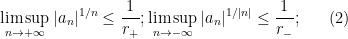
conversely, every infinite sequenceof coefficients obeying (1) arises from such a function
- (ii) Functions
are expressed by a convergent Fourier series (and also Laurent series)
, where
conversely, every doubly infinite sequenceof coefficients obeying (2) arises from such a function
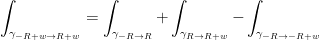
- (iii) In the situation of (ii), there is a unique decomposition
where
extends holomorphically to
, and
extends holomorphically to
and goes to zero at infinity, and are given by the formulae
whereis any anticlockwise contour in
, and and
wherebut not


This connection lets us interpret various facts about Fourier series through the lens of complex analysis, at least for some special classes of Fourier series. For instance, the Fourier inversion formula 


It turns out that there are similar links between complex analysis on a half-plane (or strip) and Fourier integrals on the real line, which we will explore in these notes.
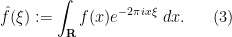
We first fix a normalisation for the Fourier transform. If 


Exercise 1 (Fourier transform of Gaussian) Ifis a complex number with
and
, show that the Fourier transform
, where we use the standard branch for
.
The Fourier transform has many remarkable properties. On the one hand, as long as the function

Exercise 2 (Decay ofHint: to establish holomorphicity in each of these cases, use Morera’s theorem and the Fubini-Tonelli theorem. For uniqueness, use analytic continuation, or (for part (iv)) the Schwartz reflection principle.
- (i) If
for all
and
(that is to say one has
for some finite quantity
depending only on
), then
. Furthermore, this function continues to be defined by (3).
- (ii) If
then the entire function
for
. In particular, if
then
.
- (iii) If
for all
, then
, and obeys the bound
in this strip. Furthermore, this function continues to be defined by (3).
- (iv) If
(resp.
), then there is a unique continuous extension of
(resp. the upper half-plane
) which is holomorphic in the interior of this half-plane, and such that
uniformly as
(resp.
). Furthermore, this function continues to be defined by (3).
Later in these notes we will give a partial converse to part (ii) of this exercise, known as the Paley-Wiener theorem; there are also partial converses to the other parts of this exercise.
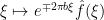
From (3) we observe the following intertwining property between multiplication by an exponential and complex translation: if 


The material in these notes is loosely adapted from Chapter 4 of Stein-Shakarchi’s “Complex Analysis”.
— 1. The inversion and Poisson summation formulae —
We now explore how the Fourier transform
Proposition 3 (Fourier transform of functions holomorphic in a strip) Let, and suppose that
which obeys a decay bound of the form
for all
,
, and some
and
(or in asymptotic notation, one has
whenever
).
- (i) (Translation intertwines with modulation) For any
in the strip
, the Fourier transform of the function
is
.
- (ii) (Exponential decay of Fourier transform) For any
such that
for all
(or in asymptotic notation, one has
for
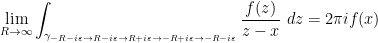
- (iii) (Partial Fourier inversion) For any
and
and
- (iv) (Full Fourier inversion) For any
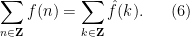
- (v) (Poisson summation formula) The identity (6) holds for this function


Proof: We begin with (i), which is a standard application of contour shifting. Applying the definition (3) of the Fourier transform, our task is to show that

 and . Clearly
 is the line segment contour from
  to
to  , and similarly after a change of variables
 . So it suffices to show that
 . But the left hand side can be rewritten as
For (ii), we apply (i) with 


 and all , giving the claim.
For the first part of (iii), we write 


 as
as  ) the left-hand side can be written as

To prove (iv), it suffices in light of (iii) to show that
 . The left-hand side can be written after a change of variables as

Now we prove (v). Let


 . If we sum the first identity for
  we see from the geometric series formula and Fubini’s theorem that
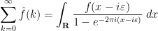
 we have


 , which are at the integers. Hence we shall restrict
  to be a half-integer
  . In this case, a routine application of the residue theorem shows that
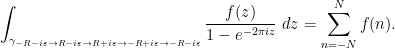
 stays bounded for in
  or
or  when is a half-integer, we also see from dominated convergence as before that

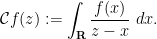
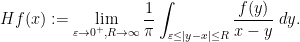
Exercise 4 (Hilbert transform and Plemelj formula) Letbe as in Proposition 3. Define the Cauchy-Stieltjes transform
by the formula
- (i) Show that
is holomorphic on
and has the Fourier representation
in the upper half-plane
and
in the lower half-plane
.
- (ii) Establish the Plemelj formulae
and
uniformly for any
of
- (iii) Show that
on
and solves the (very simple special case of the) Riemann-Hilbert problem
uniformly for all
.
- (iv) Establish the identity
where the signum function
is defined to equal
for
,
for
, and
.
- (v) Assume now that
). Show that
, and with
replaced by a slightly smaller quantity
), with the identity
holding for
. ({Hint: To exploit the mean value hypothesis to get good decay bounds on
and hence
, write
as the sum of
and
and use the mean value hypothesis to manage the first term. For the contribution of the second term, take advantage of contour shifting to avoid the singularity at
. One may have to divide the integrals one encounters into a couple of pieces and estimate each piece separately.)
- (vi) Continue to assume that
and
(Hint: for the latter inequality, square both sides of (9) and use (iii).)


Exercise 5 (Kramers-Kronig relations) Letwhich is holomorphic on the interior of this half-plane, and obeys the bound
for all non-zero
and
relating the real and imaginary parts of


Exercise 6
- (i) By applying the Poisson summation formula to the function
, establish the identity
for any positive real number
- (ii) By carefully taking limits of (i) as
, establish yet another alternate proof of Euler’s identity


Exercise 7 Forin the upper half-plane
, define the theta function
. Use Exercise 1 and the Poisson summation formula to establish the modular identity
for such

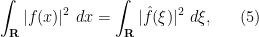
Exercise 8 (Fourier proof of Plancherel identity) Let, define the quantity
Remarkably, this proof of the Plancherel identity generalises to a nonlinear version involving a trace formula for the scattering transform for either Schrödinger or Dirac operators. For Schrödinger operators this was first obtained (implicitly) by Buslaev and Faddeev, and later more explicitly by Deift and Killip. The version for Dirac operators more closely resembles the linear Plancherel identity; see for instance the appendix to this paper of Muscalu, Thiele, and myself. The quantity
- (i) When
. (Hint: find a way to rearrange the expression
.)
- (ii) For
, where the implied constant in the
- (iii) Establish the Plancherel identity (5) (Hint: use contour shifting.).
is a component of a nonlinear quantity known as the transmission coefficient
of a Dirac operator with potential
, depending on normalisations).

The Fourier inversion formula was only established in Proposition 3 for functions that had a suitable holomorphic extension to a strip, but one can relax the hypotheses by a limiting argument. Here is one such example of this:
Exercise 9 (More general Fourier inversion formula) Letfor all

 , with
  for any
Exercise 10 (Laplace inversion formula) Letbe a continuously twice differentiable function, obeying the bounds
for all
and some
The Laplace-Mellin inversion formula in fact holds under more relaxed decay and regularity hypotheses than the ones given in this exercise, but we will not pursue these generalisations here. The limiting integral in (10) is also known as the Bromwich integral, and often written (with a slight abuse of notation) as
- (i) Show that the Fourier transform
for any non-zero
- (ii) Establish the principal value inversion formula
for any positive real
- (iii) Define the Laplace transform
of
by the formula
Show that
is continuous on the half-plane
, holomorphic on the interior of this half-plane, and obeys the Laplace-Mellin inversion formula
for any
and
, where
is the line segment contour from
to
. Conclude in particular that the Laplace transform
is injective on this class of functions
. The Laplace transform is a close cousin of the Fourier transform that has many uses; for instance, it is a popular tool for analysing ordinary differential equations on half-lines such as


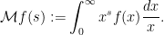
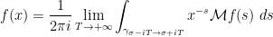
Exercise 11 (Mellin inversion formula) Letbe a continuous function that is compactly supported in
. Define the Mellin transform
by the formula
Show that
is entire and one has the Mellin inversion formula
for any
. The regularity and support hypotheses on
Exercise 12 (Perron’s formula) Letbe a function which is of subpolynomial growth in the sense that
for all
and
, where
depends on
(and
in the half-plane
, form the Dirichlet series
For any non-integer
and any
, establish Perron’s formula
What happens when


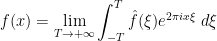
Exercise 13 (Solution to Schrödinger equation) Letbe as in Proposition 3. Define the function
by the formula \{ u(t,x) := \int_R \hat f(\xi) e^{2\pi i x \xi – 4 \pi^2 i \xi^2 t} d\xi.\}
- (i) Show that
that obeys the Schrödinger equation
with initial condition
for
- (ii) Establish the formula
for
, where we use the standard branch of the square root.

— 2. Phragmén-Lindelöf and Paley-Wiener —
The maximum modulus principle (Exercise 26 from 246A Notes 1) for holomorphic functions asserts that if a function continuous on a compact subset 


Theorem 14 (Lindelöf’s theorem) Letfor some
, which is holomorphic in the interior of the strip and obeys the bound
for all
and some constants
. Suppose also that
and
for all
and some
for all
and

Remark 15 The hypothesis (12) is a qualitative hypothesis rather than a quantitative one, since the exact values ofdo not show up in the conclusion. It is quite a mild condition; any function of exponential growth in
, or even with such super-exponential growth as
or
, will obey (12). The principle however fails without this hypothesis, as discussed previously.
Proof: By shifting and dilating (adjusting 


Suppose we temporarily assume that 


To remove the assumption that 


Corollary 16 (Phragmén-Lindelöf principle in a sector) Letfor some
, which is holomorphic on the interior of the sector and obeys the bound
for some
and
. Suppose also that
on the boundary of the sector
. Then one also has

Proof: Apply Theorem 14 to the function 

Exercise 17 With the notation and hypotheses of Theorem 14, show that the functionis log-convex on
Exercise 18 (Hadamard three-circles theorem) Let. Show that the function
is log-convex on
.
Exercise 19 (Phragmén-Lindelöf principle) Let, but with the hypotheses after “Suppose also” in that theorem replaced instead by the bounds
and
for all
and a constant
for all
(which is allowed to depend on the constants
in (12), as well as
). (Hint: it is convenient to work first in a half-strip such as
for some large
. Then multiply
for some suitable branch of the logarithm and apply a variant of Theorem 14 for the half-strip. A more refined estimate in this regard is due to Rademacher.) This particular version of the principle gives the convexity bound for Dirichlet series such as the Riemann zeta function. Bounds which exploit the deeper properties of these functions to improve upon the convexity bound are known as subconvexity bounds and are of major importance in analytic number theory, which is of course well outside the scope of this course.
Now we can establish a remarkable converse of sorts to Exercise 2(ii) known as the Paley-Wiener theorem, that links the exponential growth of (the analytic continuation) of a function with the support of its Fourier transform:
Theorem 20 (Paley-Wiener theorem) Letfor all
. Then the following are equivalent:
- (i) The Fourier transform
- (ii)
for some
.
- (iii)
for some

The continuity and decay hypotheses on
Proof: If (i) holds, then by Exercise 9, we have the inversion formula (4), and the claim (iii) then holds by a slight modification of Exercise 2(ii). Also, the claim (iii) clearly implies (ii).
Now we see why (iii) implies (i). We first assume that we have the stronger bound 

 and
and  . Applying (14) and the triangle inequality, we see that
 , we can then send
  and conclude that
  ; similarly for
  we can send
  and again conclude
  . This establishes (i) in this case.
Now suppose we only have the weaker bound on 


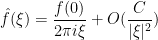
Finally, we show that (ii) implies (iii). The function 


— 3. The Hardy uncertainty principle —
Informally speaking, the uncertainty principle for the Fourier transform asserts that a function
 and all
  , which we will not prove here (see for instance Exercise 47 of this previous set of lecture notes).
Another manifestation of the uncertainty principle is the following simple fact:
Lemma 21
- (i) If
for all
, then the Fourier transform
is discrete).
- (ii) If
Proof: For (i), we observe from Exercise 2(iii) that
Lemma 21(ii) rules out the existence of a bump function whose Fourier transform is also a bump function, which would have been a rather useful tool to have in harmonic analysis over the reals. (Such functions do exist however in some non-archimedean domains, such as the 
Theorem 22 (Hardy uncertainty principle) Letfor all
for all
. Then
is a scalar multiple of the gaussian
, that is to say one has
for some
.
Proof: By replacing 


From Exercise 2(i),
 . Completing the square
  and using
  , we conclude the bound

 is bounded by on the imaginary axis. On the other hand, from hypothesis
  is also bounded by on the real axis. We can now almost invoke the Phragmén-Lindelöf principle (Corollary 16) to conclude that is bounded on all four quadrants, but the growth bound we have (15) is just barely too weak. To get around this we use the epsilon of room trick. For any , the function
  is still entire, and is still bounded by in magnitude on the real line. From (15) we have
  on the slightly tilted imaginary axis
  . We can now apply Corollary 16 in the two acute-angle sectors between
  and
and  to conclude that
  in those two sectors; letting , we conclude that
  in the first and third quadrants. A similar argument (using negative values of ) shows that in the second and fourth quadrants. By Liouville’s theorem, we conclude that is constant, thus we have
  for some complex number
  . The claim now follows from the Fourier inversion formula (Proposition 3(iv)) and Exercise 1.
One corollary of this theorem is that if 


Exercise 23 Iffor some
and
for some
for some polynomial
of degree at most
Exercise 24 In this exercise we develop an alternate proof of (a special case of) the Hardy uncertainty principle, which can be found in the original paper of Hardy. Let the hypotheses be as in Theorem 22.It is possible to adapt this argument to also cover the case of general
- (i) Show that the function
is holomorphic on the region
and obeys the bound
in this region, where we use the standard branch of the square root.
- (ii) Show that the function
is holomorphic on the region
and obeys the bound
in this region.
- (iii) Show that
agree on their common domain of definition.
- (iv) Show that the functions
are constant. (You may find Exercise 13 from 246A Notes 4 to be useful.)
- (v) Use the above to give an alternate proof of Theorem 22 in the case when
vanish. Conclude that the Taylor series coefficients of
Exercise 25 (This problem is due to Tom Liggett; see this previous post.) Letbe a sequence of complex numbers bounded in magnitude by some bound
obeys the bound
for all
and some
- (i) Show that the Laplace transform
extends holomorphically to the region
and obeys the bound
in this region.
- (ii) Show that the function
is holomorphic in the region
, obeys the bound
in this region, and agrees with
- (iii) Show that
.
- (iv) Show that the sequence
is a constant multiple of the sequence
.
Remark 26 There are many further variants of the Hardy uncertainty principle. For instance we have the following uncertainty principle of Beurling, which we state in a strengthened form due to Bonami, Demange, and Jaming: if, then

37 comments
Comments feed for this article
23 January, 2021 at 1:13 pm
Michele Nardelli, Antonio Nardelli
Dear Terence,
The topic of this very interesting post, can be applied also to the some sectors of theoretical physics? Regards
26 January, 2021 at 5:41 am
DiscoverReality Clover
Yes. I think that it is possible. It seems possible to conjecture that, based on this bound, there is a minimum pressure for a de-pressurising thermal system.
For example, based on this, one can show that if you pop a pressurised balloon (thermal system) in a vacuum then it obeys Newton’s first law – a body stays in motion… – by showing that the pressure inside the balloon does not go to zero. It approaches a minimum, hence the balloon stays in motion.
26 January, 2021 at 5:59 am
Anonymous
Thank you very much! Regards
23 January, 2021 at 2:50 pm
Anonymous
Typos in third bullet point: the integral sign in the wrong place.
[Corrected, thanks – T.]
23 January, 2021 at 2:51 pm
Anonymous
At the beginning for and
and  .
.
24 January, 2021 at 3:40 pm
Anonymous
Typo in
in 
[Corrected – T.]
23 January, 2021 at 5:47 pm
Anonymous
In the introduction of this notes, I am not sure about the proof of the “conversely” direction in (i),(ii),(iii). It is not intuitive for a sequence to satisfy certain property that it has to arise from a series of a particular form. How do we prove such statement? Say the converse direction in (i)? (Sorry, should have asked about Exe.5 from notes 4 last quarter).
[These are immediate from Proposition 7 and Theorem 15 from Notes 1 of the previous quarter’s notes. -T]
23 January, 2021 at 9:56 pm
Anonymous
Hello,
In the point (iii) there is a typo for defn of f_1 and f_2. 2πi should replace by 1/2πi and unfortunately integral signs are not in right pisition.
24 January, 2021 at 12:20 pm
Anonymous
Dear Prof. Tao
I’ve read this your very interesting Note. What other note or papers of yours can you recommend me to consult in order to delve into these interesting topics? I’m grateful if You can show/suggest me other Your papers regarding this subject, All my best wishes for your works and all my esteem and gratitude,
All the best
25 January, 2021 at 1:20 pm
Anonymous
A simple heuristic interpretation of Poisson summation formula (6) is by observing that it can be written as
(6′)
where is a nonnegative (singular) measure supported on the integers and has a unit measure on each integer.
It is not difficult to verify that is invariant under the Fourier transform, so (6′) is equivalent to
(6”)
Which (at least heuristically) follows from Plancherel’s theorem on the invariance of inner products in under Fourier transform.
5 February, 2021 at 8:47 am
N is a number
This is nice! Thank you.
25 January, 2021 at 5:27 pm
Anonymous
Title of this notes: “factorisation” should be factorization.
26 January, 2021 at 12:22 pm
Anonymous
This is for 246B, Notes 1: —
26 January, 2021 at 8:50 am
DiscoverReality Clover
Dear All,
I apologise for accidentally rating my own comment – an action which l couldn’t undo.
28 January, 2021 at 12:47 pm
Anonymous
It is interesting to observe that both the Fourier and Hilbert transforms, as linear operators on , have the property that their fourth power is the identity operator.
28 January, 2021 at 1:48 pm
Anonymous
Hi Terence Tao. I am only 14, but I understand the fundamentals of this maths work. Please can you teach me more about this. Thank you
2 February, 2021 at 4:36 am
Jim Hefferon
Not about this article. The link to “Cult of Genius” in the sidebar has changed. A litle googling found that it is now https://www.discovermagazine.com/mind/the-cult-of-genius. Regards.
[Corrected, thanks – T.]
5 February, 2021 at 8:46 am
N is a number
Just some nitpicking: in point ii towards the beginning of the post, one should have .
.
[Corrected, thanks – T.]
5 February, 2021 at 6:34 pm
Anonymous
At the end of today’s lecture, you mentioned that Fourier transform is the rotation of the function by 90 degrees in phase space, which gives a good interpretation that take Fourier transform 4 times gets back the original function. Detailed proof involves micro local analysis and something about symplectic structure. Could you provide some reference on this topic? It is a very interesting subject.
6 February, 2021 at 10:56 am
Terence Tao
In the physics literature this is known as the phase space formulation of quantum mechanics, and the Wigner quasiprobability distribution can be used as a candidate for the “phase space transform” of a function, though it is not the only such choice. A more mathematical treatment of some of these ideas can be found in Folland’s “Harmonic analysis in phase space”.
9 February, 2021 at 9:28 am
N is a number
Doesn’t the proof of Exercise 2 part i follow directly by putting to be a complex number and then utilising the super-exponential decay of
  to obtain a bound for the integral displayed on the RHS of equation 3 (for instance by using the dominated convergence theorem), and then conclude that
  defined in this way will be entire by observing that what we did actually implies that
  has no poles or other types of singularities.
9 February, 2021 at 9:41 am
N is a number
Or once we define in this way, we can also use the second funadamental theorem of calculus to obtain the claim.
9 February, 2021 at 8:37 pm
Aditya Guha Roy
I think what you wrote above is correct, and then we can use the second fundamental theorem of calculus to conclude that defined in this way will be holomorphic.
9 February, 2021 at 11:39 am
Anonymous
You mentioned in class yesterday that we use Harr measure for the Mellin transform on the half line because Harr measure is scaling invariant, and Lebesgue measure is translation invariant. Translation invariant property is more useful on the whole real line, and not very useful on the half line. Please elaborate on this. Don’t we define the Laplace transform on the half line using Lebesgure measure?
9 February, 2021 at 6:08 pm
Terence Tao
One can still try to exploit translation invariance on the half-line, but one picks up additional terms at the boundary which complicate things a little. Compare for instance the effects of differentiation or translation on the Laplace transform displayed in the table in https://en.wikipedia.org/wiki/Laplace_transform#Properties_and_theorems with the corresponding properties for the Fourier transform in https://en.wikipedia.org/wiki/Fourier_transform#Basic_properties .
10 February, 2021 at 8:26 am
Aditya Guha Roy
In ii of Exercise 2 shouldn’t we have instead of
  ?
?
[As it turns out, one does not need a dependence on here. -T]
10 February, 2021 at 8:36 am
Aditya Guha Roy
In ii of Exercise 2 I think we should have ….. .
….. .
[Here we use to denote the estimate
  (that is, the absolute values are implicit in the notation) -T.]
12 February, 2021 at 9:39 am
246B, Notes 4: The Riemann zeta function and the prime number theorem | What's new
[…] function for imaginary values of the argument in the upper half-plane (so ); from Exercise 7 of Notes 2 we have the modularity […]
13 February, 2021 at 6:01 am
Aditya Guha Roy
In the 4th line of the proof of part (iv.) in Proposition 3, the second integral should be over .
.
[Corrected, thanks – T.]
13 February, 2021 at 6:05 am
N is a number
Here we see a proof of the Fourier inversion theorem which becomes easy if one uses the tools from complex analysis as demonstrated above in the proof of Proposition 3.
We also know that for the discrete setting we can give a proof of the Fourier inversion formula which uses some algebraic manipulations and orthogonality properties.
In general is there a unified approach to prove Fourier inversion type results?
14 February, 2021 at 10:28 am
Terence Tao
There are various ways to establish Plancherel’s theorem (which includes the Fourier inversion formula as a component) on arbitrary locally compact abelian (LCA) groups; see Section 4 of these notes for a brief discussion of two approaches, one using Gelfand theory, and another via Bochner’s theorem. For special groups such as the real line or the circle there are shortcuts available that utilise special features of those groups, such as the presence of gaussians or holomorphic extensions to various regions of the complex plane, but these do not seem to generalise well to the LCA setting, which seems to be the most natural framework in which to present Fourier analysis in a unified manner.
18 February, 2021 at 5:32 pm
Anonymous
About the Beurling uncertainty principle [Remark 26], how do you get the hyperbola geometric interpretation phase portrait? Does it follow directly from the square integrability condition? I know and
and  are kind of “inverse” to each other.
[It arises from consideration of where the weight is exponentially large. -T.]
27 February, 2021 at 9:14 am
Course announcement: 246B, complex analysis | What's new
[…] Connections with the Fourier transform on the real line; […]
27 February, 2021 at 9:36 am
246B, Notes 1: Zeroes, poles, and factorisation of meromorphic functions | What's new
[…] Previous set of notes: 246A Notes 5. Next set of notes: Notes 2. […]
27 February, 2021 at 9:38 am
246B, Notes 3: Elliptic functions and modular forms | What's new
[…] set of notes: Notes 2. Next set of notes: Notes […]
18 January, 2022 at 1:38 am
Quan
Dear Professor Tao,
In the Laplace transform problem, one comes up with a different restriction for {f} that {f} is continuously differentiable and {\vert f(x)e^{-xt}\vert \leq \frac{C_t}{1+x^2}, \forall t \in {\bf R} (1)}. Then, we construct a compactly supported function {h(x)} that agrees with {2\pi f(2\pi x)e^{-2\pi xt}} when {x\geq 0} for the purpose of applying Fourier transform (modify the proof of excercise 9 for function with contable discontinuities), and one can obtain the Laplace transform for the class of function satisfies (1). Is this approach valid? Thank you for your time, professor.
[Large parts of Exercise 10 would still be valid under these more general hypotheses on , though perhaps not all. It would be a instructive exercise for you to work out the details. -T]
24 January, 2022 at 1:38 pm
Quân Nguyễn
I think the proof that Exercise 9 can still be applied for the Laplace inverse transform (exercise 10) if we withdraw the condition of $f$ being differentiable.