
In my previous post, I walked through the task of formally deducing one lemma from another in Lean 4. The deduction was deliberately chosen to be short and only showcased a small number of Lean tactics. Here I would like to walk through the process I used for a slightly longer proof I worked out recently, after seeing the following challenge from Damek Davis: to formalize (in a civilized fashion) the proof of the following lemma:
Lemma. Let
and
be sequences of real numbers indexed by natural numbers
, with
non-increasing and
non-negative. Suppose also that
for all
. Then
for all
.
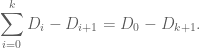
Here I tried to draw upon the lessons I had learned from the PFR formalization project, and to first set up a human readable proof of the lemma before starting the Lean formalization – a lower-case “blueprint” rather than the fancier Blueprint used in the PFR project. The main idea of the proof here is to use the telescoping series identity
Since 

but by the monotone hypothesis on 

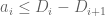
This is already a human-readable proof, but in order to formalize it more easily in Lean, I decided to rewrite it as a chain of inequalities, starting at 

(by field identities)

(by the formula for summing a constant)

(by the monotone hypothesis)

(by the hypothesis
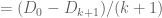
(by telescoping series)

(by the non-negativity of
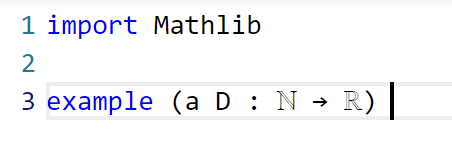
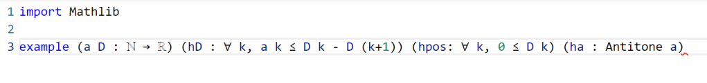
I decided that this was a good enough blueprint for me to work with. The next step is to formalize the statement of the lemma in Lean. For this quick project, it was convenient to use the online Lean playground, rather than my local IDE, so the screenshots will look a little different from those in the previous post. (If you like, you can follow this tour in that playground, by clicking on the screenshots of the Lean code.) I start by importing Lean’s math library, and starting an example of a statement to state and prove:

Now we have to declare the hypotheses and variables. The main variables here are the sequences a, D from the natural numbers ℕ to the reals ℝ. (One can choose to “hardwire” the non-negativity hypothesis into the D take values in the nonnegative reals 
NNReal in Lean), but this turns out to be inconvenient, because the laws of algebra and summation that we will need are clunkier on the non-negative reals (which are not even a group) than on the reals (which are a field). So we add in the variables:
Now we add in the hypotheses, which in Lean convention are usually given names starting with h. This is fairly straightforward; the one thing is that the property of being monotone decreasing already has a name in Lean’s Mathlib, namely Antitone, and it is generally a good idea to use the Mathlib provided terminology (because that library contains a lot of useful lemmas about such terms).
One thing to note here is that Lean is quite good at filling in implied ranges of variables. Because a and D have the natural numbers ℕ as their domain, the dummy variable k in these hypotheses is automatically being quantified over ℕ. We could have made this quantification explicit if we so chose, for instance using ∀ k : ℕ, 0 ≤ D k instead of ∀ k, 0 ≤ D k, but it is not necessary to do so. Also note that Lean does not require parentheses when applying functions: we write D k here rather than D(k) (which in fact does not compile in Lean unless one puts a space between the D and the parentheses). This is slightly different from standard mathematical notation, but is not too difficult to get used to.
This looks like the end of the hypotheses, so we could now add a colon to move to the conclusion, and then add that conclusion:

This is a perfectly fine Lean statement. But it turns out that when proving a universally quantified statement such as ∀ k, a k ≤ D 0 / (k + 1), the first step is almost always to open up the quantifier to introduce the variable k (using the Lean command intro k). Because of this, it is slightly more efficient to hide the universal quantifier by placing the variable k in the hypotheses, rather than in the quantifier (in which case we have to now specify that it is a natural number, as Lean can no longer deduce this from context):

At this point Lean is complaining of an unexpected end of input: the example has been stated, but not proved. We will temporarily mollify Lean by adding a sorry as the purported proof:

Now Lean is content, other than giving a warning (as indicated by the yellow squiggle under the example) that the proof contains a sorry.
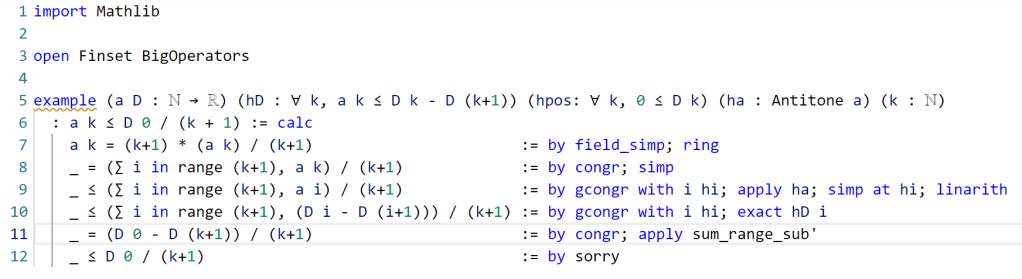
It is now time to follow the blueprint. The Lean tactic for proving an inequality via chains of other inequalities is known as calc. We use the blueprint to fill in the calc that we want, leaving the justifications of each step as “sorry”s for now:

Here, we “open“ed the Finset namespace in order to easily access Finset‘s range function, with range k basically being the finite set of natural numbers 
open“ed the BigOperators namespace to access the familiar ∑ notation for (finite) summation, in order to make the steps in the Lean code resemble the blueprint as much as possible. One could avoid opening these namespaces, but then expressions such as ∑ i in range (k+1), a i would instead have to be written as something like Finset.sum (Finset.range (k+1)) (fun i ↦ a i), which looks a lot less like like standard mathematical writing. The proof structure here may remind some readers of the “two column proofs” that are somewhat popular in American high school geometry classes.
Now we have six sorries to fill. Navigating to the first sorry, Lean tells us the ambient hypotheses, and the goal that we need to prove to fill that sorry:

The ⊢ symbol here is Lean’s marker for the goal. The uparrows ↑ are coercion symbols, indicating that the natural number k has to be converted to a real number in order to interact via arithmetic operations with other real numbers such as a k, but we can ignore these coercions for this tour (for this proof, it turns out Lean will basically manage them automatically without need for any explicit intervention by a human).
The goal here is a self-evident algebraic identity; it involves division, so one has to check that the denominator is non-zero, but this is self-evident. In Lean, a convenient way to establish algebraic identities is to use the tactic field_simp to clear denominators, and then ring to verify any identity that is valid for commutative rings. This works, and clears the first sorry:

field_simp, by the way, is smart enough to deduce on its own that the denominator k+1 here is manifestly non-zero (and in fact positive); no human intervention is required to point this out. Similarly for other “clearing denominator” steps that we will encounter in the other parts of the proof.
Now we navigate to the next `sorry`. Lean tells us the hypotheses and goals:

We can reduce the goal by canceling out the common denominator ↑k+1. Here we can use the handy Lean tactic congr, which tries to match two sides of an equality goal as much as possible, and leave any remaining discrepancies between the two sides as further goals to be proven. Applying congr, the goal reduces to

Here one might imagine that this is something that one can prove by induction. But this particular sort of identity – summing a constant over a finite set – is already covered by Mathlib. Indeed, searching for Finset, sum, and const soon leads us to the Finset.sum_const lemma here. But there is an even more convenient path to take here, which is to apply the powerful tactic simp, which tries to simplify the goal as much as possible using all the “simp lemmas” Mathlib has to offer (of which Finset.sum_const is an example, but there are thousands of others). As it turns out, simp completely kills off this identity, without any further human intervention:

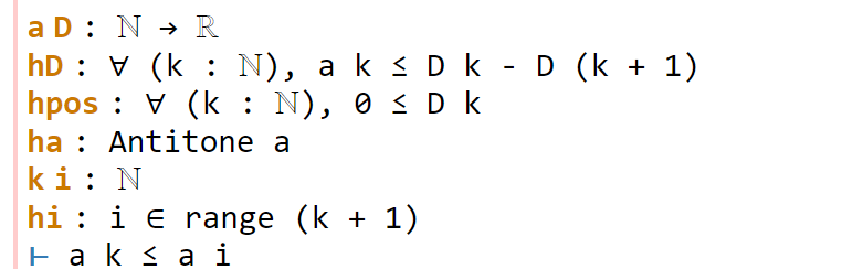
Now we move on to the next sorry, and look at our goal:

congr doesn’t work here because we have an inequality instead of an equality, but there is a powerful relative gcongr of congr that is perfectly suited for inequalities. It can also open up sums, products, and integrals, reducing global inequalities between such quantities into pointwise inequalities. If we invoke gcongr with i hi (where we tell gcongr to use i for the variable opened up, and hi for the constraint this variable will satisfy), we arrive at a greatly simplified goal (and a new ambient variable and hypothesis):
Now we need to use the monotonicity hypothesis on a, which we have named ha here. Looking at the documentation for Antitone, one finds a lemma that looks applicable here:
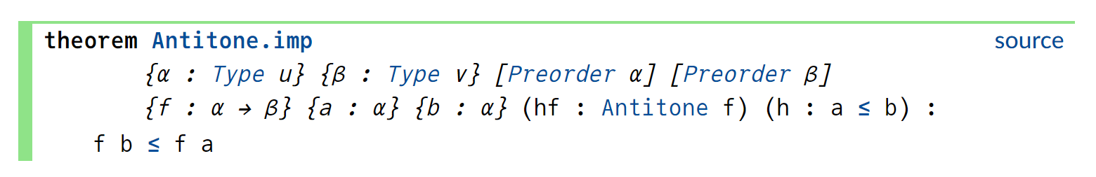
One can apply this lemma in this case by writing apply Antitone.imp ha, but because ha is already of type Antitone, we can abbreviate this to apply ha.imp. (Actually, as indicated in the documentation, due to the way Antitone is defined, we can even just use apply ha here.) This reduces the goal nicely:

The goal is now very close to the hypothesis hi. One could now look up the documentation for Finset.range to see how to unpack hi, but as before simp can do this for us. Invoking simp at hi, we obtain

Now the goal and hypothesis are very close indeed. Here we can just close the goal using the linarith tactic used in the previous tour:

The next sorry can be resolved by similar methods, using the hypothesis hD applied at the variable i:

Now for the penultimate sorry. As in a previous step, we can use congr to remove the denominator, leaving us in this state:
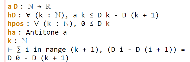
This is a telescoping series identity. One could try to prove it by induction, or one could try to see if this identity is already in Mathlib. Searching for Finset, sum, and sub will locate the right tool (as the fifth hit), but a simpler way to proceed here is to use the exact? tactic we saw in the previous tour:

A brief check of the documentation for sum_range_sub' confirms that this is what we want. Actually we can just use apply sum_range_sub' here, as the apply tactic is smart enough to fill in the missing arguments:
One last sorry to go. As before, we use gcongr to cancel denominators, leaving us with

This looks easy, because the hypothesis hpos will tell us that D (k+1) is nonnegative; specifically, the instance hpos (k+1) of that hypothesis will state exactly this. The linarith tactic will then resolve this goal once it is told about this particular instance:

We now have a complete proof – no more yellow squiggly line in the example. There are two warnings though – there are two variables i and hi introduced in the proof that Lean’s “linter” has noticed are not actually used in the proof. So we can rename them with underscores to tell Lean that we are okay with them not being used:

This is a perfectly fine proof, but upon noticing that many of the steps are similar to each other, one can do a bit of “code golf” as in the previous tour to compactify the proof a bit:

With enough familiarity with the Lean language, this proof actually tracks quite closely with (an optimized version of) the human blueprint.
This concludes the tour of a lengthier Lean proving exercise. I am finding the pre-planning step of the proof (using an informal “blueprint” to break the proof down into extremely granular pieces) to make the formalization process significantly easier than in the past (when I often adopted a sequential process of writing one line of code at a time without first sketching out a skeleton of the argument). (The proof here took only about 15 minutes to create initially, although for this blog post I had to recreate it with screenshots and supporting links, which took significantly more time.) I believe that a realistic near-term goal for AI is to be able to fill in automatically a significant fraction of the sorts of atomic “sorry“s of the size one saw in this proof, allowing one to convert a blueprint to a formal Lean proof even more rapidly.
One final remark: in this tour I filled in the “sorry“s in the order in which they appeared, but there is actually no requirement that one does this, and once one has used a blueprint to atomize a proof into self-contained smaller pieces, one can fill them in in any order. Importantly for a group project, these micro-tasks can be parallelized, with different contributors claiming whichever “sorry” they feel they are qualified to solve, and working independently of each other. (And, because Lean can automatically verify if their proof is correct, there is no need to have a pre-existing bond of trust with these contributors in order to accept their contributions.) Furthermore, because the specification of a “sorry” someone can make a meaningful contribution to the proof by working on an extremely localized component of it without needing the mathematical expertise to understand the global argument. This is not particularly important in this simple case, where the entire lemma is not too hard to understand to a trained mathematician, but can become quite relevant for complex formalization projects.

31 comments
Comments feed for this article
6 December, 2023 at 1:21 am
wdjoyner
Thank you for the interesting post but I think there’s a typo somewhere. After “I start by importing Lean’s math library, and starting an example of a statement to state and prove:” the display is blank.
[Added, thanks – T.]
6 December, 2023 at 2:24 am
Anonymous
Re: the twitter challenge from Damek Davis.
“You’re unable to view this Post because this account owner limits who can view their Posts. Learn more”
6 December, 2023 at 3:43 am
Dustin G. Mixon
In the second display, the sum of a_i should be leq D_0.
[Corrected, thanks – T.]
6 December, 2023 at 4:41 am
Anonymous
Isn’t it Sum a_i <= D_0 rather than =
7 December, 2023 at 12:18 am
Anonymous
All rhs have / (k + 1) in common. The proof would be simpler if we prove (k+1)a_k \le D_0 first.
7 December, 2023 at 8:18 am
Terence Tao
This is certainly an option. Here is one arrangement of the proof that follows that strategy; there is one “rewrite” inserted at the beginning, and an number of `congr` and `gcongr` steps that were used to remove the denominator are removed. I think it is roughly the same length and complexity in the end.
7 December, 2023 at 1:08 am
Anonymous
That’s fascinating Terry. What do you see as the value of golfing the code? As someone with a background in commercial programming, I’m used to trying to make code as clear and simple as possible. To my eyes, the golfed code is significantly harder to read. But I’m not a mathematician, so I may well lack the right perspective here.
7 December, 2023 at 8:14 am
Terence Tao
From the mathematical side, I think it comes down to the principle of “giving appropriate amounts of detail”, which I write about here. Ideally, each step in a proof should be of the natural size that a mathematician would interpret as a significant step towards resolving the problem, and all steps should be broadly of similar size. The initial blueprint, breaking up the proof into six very tiny steps, satisfies the second property but not the first in my opinion, whereas the golfed version containing three steps is a bit more consonant with the high-level description of the proof rather than the low-level one.
For large projects (and particularly for contributing to Mathlib, the largest project of all), code is often “golf”ed not so much for brevity as for compilation speed. Powerful and intuitive tactics such as `simp` that perform an extensive search as part of their execution are often replaced with much more explicit `low level` tactics that are much faster but also harder to read. (There is a tactic called `simp?` which runs `simp` but then prints the specific simp lemmas used, which can then be used for this sort of compilation golf.) Perhaps this practice also influences the default aesthetic that the Lean formalization community has regarding how to write proofs, in that they tend to favor compactified arguments over long discursive ones in their Lean code. I like the Blueprint model in which LaTeX is used to describe the human readable version of the proof, while Lean focuses on its strength, which is to describe the machine readable version, but there are links between the two.
7 December, 2023 at 1:01 pm
A slightly longer Lean 4 proof tour – Cyber Geeks Global
[…] Comments…Read More […]
7 December, 2023 at 1:08 pm
Richard
A thing I find off-putting about attempting to look at anything in Lean is the use of whacky 1970s-era computer language naming. Especially so with arbitrary and inconsistent abbreviations (abrvs, abbrevs, abs?) but also finSetSummand_unKnown_why_dothis.
“congr” WTF?
It’s especially difficult to navigate this salad of capitalization and arbitrary punctuation and runtgethrwds if one’s native language is not English. linear_arithmetic (better, linear-arithmetic, because normal English used by normal humans uses hypthens to join compound words) vs “linarith” or “linArith”, or God save us, “Linarith”, not only means a hell of a lot more to a casual reader, but makes it even possible for English non-adepts to *begin* to understand what’s going on, using the full words they already know because they’re actually in use in actual mathematics, aided by looking up normal words in normal dictionaries. (Yes, “linarith” is easy, but lots of other stuff, pretty much anything beyond this, really is not.)
I get that C programmers in 1970 were very concerned about every byte that the programs took up, and that naming somethign “inj” instead of “injective-functor” would save a lot of repetitive typing in the very primitive text editors of the time, but this hasn’t been the case for 40 years now … and yet computer-ese gibberish refuses to die.
I do understand that Lean itself wasn’t expressly designed for mathematics per se.
I get that it’s written by (and incredibly generously shared by) people completely steeped in decades of unpleasant computer language conventions. Do fish have a word for water?
I keep reading that Lean proofs “aren’t meant to be read” (because having computer programs, which is what Lean proofs are, be impenetrable, even at a superficial skimming level, is somehow a good thing.) But “proofs not mean to be read” are exactly what is exposed every time somebody new tries to even casually look at this formalization business.
In the end, there’s so much ancient computer programming language-ese exposed and inflicted; it’s off-putting. Trauma inflicted on each generation of computer programmers by the their preDecssrs is now inflicted more widely.
It’s truly nice that one can use finally use characters like “≺” and “⋂” and “⨂” in the future in 2023. But the “words” formed by run-together roman letters in between these familar, comprehensible operators? Oof.
Couldn’t Math_lib_hvDoneBetr? For mathematicians? It’s a tough tough slog.
7 December, 2023 at 2:38 pm
Terence Tao
Mathlib’s naming conventions are laid out in this web page. One rationale for such conventions is to be able to quickly recognize whether a given term refers to a proposition, type, variable, or tactic (much as how in English, Capitalization is used to indicate Proper Nouns, ALLCAPS is used to indicate acronyms and initialisms, periods are used to indicate abbreviations (e.g., abbrev., etc.), italics are used to denote foreign words that are used verbatim, and so forth). Another key motivation for encouraging a rather formal naming system here is to make it easier to find specific Mathlib routines that achieve specific tasks. For instance, to find the lemma that establishes the telescoping series formula , I knew from the naming conventions that the formula name should probably involve `Finset`, `sum`, `sub`, and possibly also `range` or `eq`, and indeed by entering these terms into a Mathlib search engine one can readily locate `Finset.sum_range_sub‘` which establishes precisely this fact. Naming this fact `telescoping_series_identity` or `Lemma 3.1.4.7` would make it more difficult to reliably locate the tool. (Though in a few years this issue may become moot, as AI-powered semantic search engines become more powerful, as well as AI-powered ways to convert Lean code into human-readable proofs.)
For personal Lean projects one can always introduce one’s own personal abbreviations to replace the default names given by Mathlib of course, much as one can add a personal set of macros to replace LaTeX’s default names for various mathematical symbols with names that one personally prefers.
Also, `congr` is an abbreviation of “congruence” (and `gcongr` is an abbreviation for “generalized congruence”). Hyphens can’t be used in a mathematical language as they are already reserved for subtraction: `linear-arithmetic` would be interpreted as the difference of `linear` and `arithmetic`.
7 December, 2023 at 10:58 pm
Anonymous
Thank you for making this post (all the screenshots and special Lean style must take a lot of time).
One quick question: is Lean able to look at a proof, and say, oh this proposition always works for other fields (instead of reals). Well, not very useful in this case, but hypothetically. Humans can probably spot it easily, but I wonder if you’ve had the experience that you have missed a trivial extension which was “pointed out” by Lean. Thanks!
8 December, 2023 at 7:35 am
Terence Tao
Well, Lean’s compiler has a “linter” that points out if a variable or hypothesis in the proposition was never actually used in the proof, so that is one simple way in which trivial extensions can be spotted. Another experience I have had is that sometimes, after a proposition has been proven, someone in the project realizes that in order to apply the proposition neatly in some other part of the project, one has to slightly modify a hypothesis in one of the proposition. Often one can just modify that hypothesis and watch what the compiler does. A surprisingly large fraction of the proof often still compiles under minor modifications, especially if the proof has not been prematurely optimized and one still uses broad tactics such as `simp` or `linarith` that don’t require precisely specifying all the steps, but instead lets the compiler automatically locate the hypotheses, parameters, and methods needed to resolve the problem. Generally the compiler will only throw a handful of errors under a minor modification, which can then be dealt with by hand (and the process may recurse for a few iterations, because of steps after the first error that the initial compiler run did not even reach), but with well-designed proofs, the process of modifying a proposition is often substantially easier than writing a proof from scratch. (Indeed it is this aspect of formalization where I think we really have a chance in the future of being in a situation where the task is *faster* to perform in a formal framework than in traditional pen-and-paper (and LaTeX) framework.)
8 December, 2023 at 10:58 am
Anonymous
Does it?
9 December, 2023 at 3:15 am
Tony Carbery
At the risk of introducing a red herring to the conversation, I’d be interested if there were a Lean-type proof of the following free-standing inequality involving non-negative real numbers (or alternatively non-negative integers). We have three sequences (indexed by non-negative integers
  ) and one sequence
  (indexed by triples of non-negative integers). The inequality is
where the sums are over all relevant indices, and where the quantity is given by
where the sum is over all visible indices. (The last expression is more readily visualised by writing the four terms in a vertical stack: we contract the indices 1 and 2, in the first column, indices 2 and 3 in the second column and indices 3 and 4 in the third column. This picture makes it apparent that the inequality in question is simply the case of a more general family of inequalities, the case
  of such is the Cauchy–Schwarz inequality.)
I realise this question looks really artificial and horribly technical, but I’ve not been able to find a simpler model which raises the same issues.
9 December, 2023 at 7:03 pm
Terence Tao
This is an interesting inequality – a variant of the Blakely-Roy inequality? At its current stage of development, Lean isn’t really capable of coming up with proofs on its own unless there is already a human-readable proof available already (or if a *very* short proof is available). Do you have such a human-readable proof? If so, I can take a stab at trying to formalize it. I’m guessing that the tensor power trick argument that Nets and I used to prove Lemma 2.1 of https://arxiv.org/pdf/math/9906097.pdf may give a proof that is not too difficult to formalize in Lean (which has no essential difficulty dealing with real analysis techniques such as the passage to a limit arising in the tensor power trick), but first (as in this post) one would have to write a human-readable proof first.
10 December, 2023 at 11:20 am
Anonymous
Yes, indeed, this inequality was inspired by your paper with Nets that you mention, and can indeed be proved by the tensor power trick. I was always intrigued that I couldn’t prove it “by hand” even when restricting the inputs to range over finite collections — even in this finitistic setting a limiting argument seemed to be needed. (I was hoping that a computer would one day prove it for me without recourse to limiting arguments, and, if I’m honest, that was my real motivation in asking the question here.) The human-readable proof is available at \url{https://www.ams.org/journals/proc/2004-132-11/S0002-9939-04-07565-3/?active=current}. Thanks for the heads up on Blakely-Roy, which I was sadly unaware of.
10 December, 2023 at 6:31 pm
Terence Tao
Ah, I remember this paper now. One could translate that paper step by step into Lean, but it would be rather time-consuming and not all that edifying. Lean is a formal proof assistant rather than an automatic theorem prover; it can formalize existing proofs, but at the current state of development it is not all that useful in discovering new proofs.
On the other hand, I believe one can interpret your proof through the lens of entropy inequalities, and in particular through the Legendre-Fenchel formula
for any finite set and any function
  , where the supremum is over all
  -valued random variables and
 ![{\bf H}[X] = \sum_{s \in S} {\bf P}[X=s] \log \frac{1}{{\bf P}[X=s]}](https://s0.wp.com/latex.php?latex=%7B%5Cbf+H%7D%5BX%5D+%3D+%5Csum_%7Bs+%5Cin+S%7D+%7B%5Cbf+P%7D%5BX%3Ds%5D+%5Clog+%5Cfrac%7B1%7D%7B%7B%5Cbf+P%7D%5BX%3Ds%5D%7D&bg=ffffff&fg=545454&s=0&c=20201002) is the Shannon entropy of
is the Shannon entropy of  . (This formula is perhaps more familiar to you as the duality relation between the Orlicz spaces
  and
and  .) It is then possible to prove your inequality from the Shannon entropy inequalities, without explicit use of the tensor power trick. I’ll write this up in a separate blog post.
15 December, 2023 at 6:39 pm
YahyaAA1
Terry, it’s instructive to see how you’re evolving better strategies for working with this new(ish) proof assistant tool:
‘I am finding the pre-planning step of the proof (using an informal “blueprint” to break the proof down into extremely granular pieces) to make the formalization process significantly easier than in the past (when I often adopted a sequential process of writing one line of code at a time without first sketching out a skeleton of the argument).’
You talk of using LEAN’s “tactics”. Do you think it will soon also have “strategies”, at a higher hierarchical level, perhaps as “macros” of its tactics? And that would let us “blueprint” the proof at such a level?
16 December, 2023 at 8:49 am
Terence Tao
Certainly there is work in this direction, particuarly using AI tools either in a “bottom up” fashion to develop smarter “meta-tactics” that can solve in one shot problems that currently require several lines of Lean code, or in a “top down” fashion to try to break up a long argument into smaller chunks that could then be converted to a blueprint type format. See for instance “Sagredo” or “LeanDojo” for some current experiments in the former direction. There is also the recent “FunSearch” proof of concept which gained some attention in the popular media, which perhaps is closer to the “automatic strategy generation” approach you were suggesting.
1 January, 2024 at 5:45 am
Anonymous
How is the set of natural numbers defined in Lean4?
1 January, 2024 at 7:51 am
Anonymous
For all ,
,
Also, for all ,
, 
Are both provable in Lean 3 & 4?
2 January, 2024 at 12:51 pm
Terence Tao
Sure, they are both easily provable by Lean’s `ring` tactic, see here. The natural numbers are defined in Lean as an inductive type `Nat` (or ℕ): roughly speaking, a natural number is either zero, or a successor of a natural number, and these are the only ways to produce natural numbers. (This is slightly different from the orthodox ZFC construction of the natural numbers, but ends up being functionally equivalent in practice.)
3 January, 2024 at 9:48 am
Anonymous
Many thanks for a crystal clear answer, more on the type theoretic foundation later. We are just now at the beginning of 2024.
For large mathematical objects, we have formalized so many kinds of objects in various proof assistants. In forseeable years, it seems that Coq, Lean, and Metamath will be standard among formalized mathematics.
How would we formalize the combinatorial proof of the above statement? Similarly, large formalization projects are struggling to do what everyday mathematicians can easily do: arithmetic topology.
21 January, 2024 at 7:14 pm
Terence Tao
The combinatorial statement – that the powerset of a set of cardinality n decomposes as the disjoint union of the i-element subsets for – is formalized in Lean here, and it is not difficult to then conclude the binomial identity: see here. (This identity is also implemented here.)
1 January, 2024 at 12:19 pm
Anonymous
27 January, 2024 at 2:50 am
Anonymous
The Goldbach conjecture is true becase the fractional remainders after deductions of 2/P where P= prime less than sqrt:x always end leaving may primes, short, simple absolute with a clear example demonstrating just how impossible it is not to be true.
Every even number x is always the sum of 2 prime numbers because with every increase in value of x (always 2 integers more than the last) then all odd numbers below x/2 move one further away from x/2 and all above x/2 move one closer, so the odd numbers always pair with another odd number. So if one odd number a distance k below x/2 is a multiple of a Prime (Pn) then we can rule out it and the number a distance k above x/2 as being a prime pair. So by eliminating all multiples of P<√x we can figure out how many primes will be left over and these must pair, add together to equal x. We do this by dividing x by 2 to get the number of odd numbers below x then subtract 2 by all multiples of primes <√x which is any remaining number divided by 2/P where P is the next higher prime eg:
There are always more primes left over below and above x/2 after such pairings have been eliminated (as demonstrated in this example below where x=10,004 which is illustrative for all values of x) so those primes remaining must be prime pairs. So the Goldbach conjecture is definitely true.
To demonstrate that with an example let's look at a number with no prime factors to get the least possible number of possible prime pairs
X=10,004/2=5000
5000×2/3=333.33333
333.33333×2/5=2,666.6666
2,666.6666×2/7=1904.76184
1904.76184×2/11=346.32033 =
1,558.44151-2/13=1318.6812776923 1,318.6812776923'-2/17=155.13897
1,163.542303846-2/19=1,041.0641665991
1,041.0641665991-2/23=950.5368477644
950.5368477644-2/29=884.9825824058
884.9825824058-2/31=827.8869319542
827.8869319542-2/37=783.1362870353
783.1362870353-2/41=744.934516936
744.934516936-2/43=710.2863998692
710.2863998692-2/47=680.0614466833
680.0614466833-2/53=654.3998826575
654.3998826575-2/59=632.2168357878
632.2168357878-2/61=611.4884149423
611.4884149423-2/67=593.2350294216
593.2350294216-2/71=576.5241835224
576.5241835224-2/73=560.7290004122
560.7290004122-2/79=546.5333295157
546.5333295157-2/83=533.363851696
533.363851696-2/89=521.3781471635
521.3781471635-2/97=510.6280822735
That's all primes <√x
Even if we were to include multiples of primes greater than <√x and even as the values of x go towards gazillions of gazillions of bazillions and beyond the figure will eventually converge to a percentage of x much higher than 2 for one Prime pair as the trend below demonstrates, note, primes above <√x are not relevant, I just include these to emphasise how impossible it is to not have prime pairs=x and the higher the value of x the greater the number of prime pairs will be left
510.6280822735-2/101=500.5166350998
500.5166350998-2/103=490.7978654862
490.7978654862-2/107=481.624073608
481.624073608-2/109=472.7869346427
472.7869346427-2/113=464.419024295
464.419024295-2/127=457.105338873
457.105338873-2/131=450.1266314093
450.1266314093-2/137=443.5554397099
443.5554397099-2/139=437.1733470522
437.1733470522-2/149=431.305248434
431.305248434-2/151…..etc
This and my proof to the Collatz conjecture with voiceover for visually impaired are in a mathematical proof playlist on my youtube channel Sean A Gilligan maths & physics.
27 January, 2024 at 4:57 am
lucyeinsteinbfca8f877e
Made an error in the previous comment and dont know how to delelete it sorry, of topic but homeless and unable to access the peer review system so puttng it here for obvious reasons. Thanks Terry
Fatigue is a killer! I made one error in this proof and it messed up all further numbers, here it is fixed. The proof to the Goldbach conjecture. Please take it with the level of seriousness it warrants and share.
The Goldbach conjecture is true, every even number x is always the sum of 2 prime numbers because with every increase in value of x (always 2 integers more than the last) then all odd numbers below x/2 move one further away from x/2 and all above x/2 move one closer, so the odd numbers always pair with another odd number. So if one odd number a distance k below x/2 is a multiple of a Prime (Pn) then we can rule out it and the number a distance k above x/2 as being a prime pair. So by eliminating all multiples of P<√x we can figure out how many primes will be left over and these must pair, add together to equal x. We do this by dividing x by 2 to get the number of odd numbers below x then subtract 2 by all multiples of primes <√x which is any remaining number divided by 2/P where P is the next higher prime eg:
There are always more primes left over below and above x/2 after such pairings have been eliminated (as demonstrated in this example below where x=10,004 which is illustrative for all values of x) so those primes remaining must be prime pairs. So the Goldbach conjecture is definitely true.
To demonstrate that with an example let's look at a number with no prime factors to get the least possible number of possible prime pairs
X=10,004/2=5002
5002-2/3=5,002−((5,002)×(2/3)=
1,667.3333333333-2/5=1000.4
1000.4-2/7=714.5714285714
714.5714285714-2/11=584.6493506493
584.6493506493-2/13=494.7032967033
494.7032967033-2/17=436.5029088559
436.5029088559-2/19=390.5552342395
390.5552342395-2/23=356.593909523
356.593909523-2/29=332.0012261076
332.0012261076-2/31=310.5817921652
310.5817921652-2/37=293.7935871833
293.7935871833-2/41=279.4621926866
279.4621926866-2/43=266.4639511663
266.4639511663-2/47=255.1250596273
255.1250596273-2/53=245.4976988866
245.4976988866-2/59=237.1757429921
237.1757429921-2/61=229.3994891235
229.3994891235-2/67=222.5517431795
222.5517431795-2/71=216.2826799913
216.2826799913-2/73=210.3571271148
210.3571271148-2/79=205.0316302258
205.0316302258-2/83=200.0911090155
200.0911090155-2/89=195.5946795994
195.5946795994-2/97=191.5617996077
That's less all multiples of primes <√x where x=10,004 not even allowing for some odds which are not primes to pair up, which they will and still we get a MINIMUM of around 95 prime pairs adding to x
Even if we were to include multiples of primes greater than <√x and even as the values of x go towards gazillions of gazillions of bazillions and beyond the figure will eventually converge to a percentage of x much higher than 2 for one Prime pair which further emphasises just how impossible it is to not have prime pairs adding to x.
This and my proof to the Collatz conjecture are also in short video format usually about 3 to 5 minutes, with voiceover for visually impaired in a mathematical proof playlist on my youtube channel Sean A Gilligan maths & physics.
29 January, 2024 at 7:02 am
Anonymous
Claim: Every infinite computably enumerable set has an infinite computable subset.
Proof: Consider a computably enumerable set where
where  . Define the following order in
  : for two strings
  , we say
  if either
  (where
  denotes the length of the string
  ), or
), or  and
and  (i.e.
(i.e.  precedes
  in the usual lexicographic order).
So some computable enumerator of enumerates
  as a list:
  . Call an
  a pioneer if either
  (well, the very first one is always a pioneer), or
  and
and  (
( beats all the so-far-enumerated ones). Let
  . Clearly,
  .
.
Note that the subsequence of pioneers is strictly increasing. Eventually, the latest pioneer must be greater than . So,
. So,  is accepted if and only if it is a pioneer at some time in the timeline. For us,
  is computable.
Strictly mathematically put, we should call an index a pioneer index instead of
  , but for an easy-to-understand manner, we did it as above.
16 February, 2024 at 12:16 pm
Anonymous
Hey Tao, just wanted to say your post has inspired me to learn Lean and I am loving it. Thanks!
15 April, 2024 at 2:02 am
Theorem Proving using Machine Learning – Lean 4 – A Guide To Mathematical Studies
[…] Formalizing the proof of PFR in Lean4 using Blueprint: a short tour A slightly longer Lean 4 proof tour […]