Inverting the Schur complement, and large-dimensional Gelfand-Tsetlin patterns

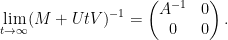
Suppose we have an matrix that is expressed in block-matrix form as

where is an matrix, is an matrix, is an matrix, and is a matrix for some . If is invertible, we can use the technique of Schur complementation to express the inverse of (if it exists) in terms of the inverse of , and the other components of course. Indeed, to solve the equation

where are column vectors and are column vectors, we can expand this out as a system

Using the invertibility of , we can write the first equation as

and substituting this into the second equation yields

and thus (assuming that is invertible)

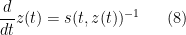
and then inserting this back into (1) gives

Comparing this with

we have managed to express the inverse of as

One can consider the inverse problem: given the inverse of , does one have a nice formula for the inverse of the minor ? Trying to recover this directly from (2) looks somewhat messy. However, one can proceed as follows. Let denote the matrix

(with the identity matrix), and let be its transpose:

Then for any scalar (which we identify with times the identity matrix), one has

and hence by (2)

noting that the inverses here will exist for large enough. Taking limits as , we conclude that

On the other hand, by the Woodbury matrix identity (discussed in this previous blog post), we have

and hence on taking limits and comparing with the preceding identity, one has

This achieves the aim of expressing the inverse of the minor in terms of the inverse of the full matrix. Taking traces and rearranging, we conclude in particular that

In the case, this can be simplified to

where is the basis column vector.

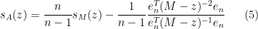
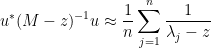
We can apply this identity to understand how the spectrum of an random matrix relates to that of its top left minor . Subtracting any complex multiple of the identity from (and hence from ), we can relate the Stieltjes transform of with the Stieltjes transform of :

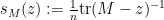
At this point we begin to proceed informally. Assume for sake of argument that the random matrix is Hermitian, with distribution that is invariant under conjugation by the unitary group ; for instance, could be drawn from the Gaussian Unitary Ensemble (GUE), or alternatively could be of the form for some real diagonal matrix and a unitary matrix drawn randomly from using Haar measure. To fix normalisations we will assume that the eigenvalues of are typically of size . Then is also Hermitian and -invariant. Furthermore, the law of will be the same as the law of , where is now drawn uniformly from the unit sphere (independently of ). Diagonalising into eigenvalues and eigenvectors , we have

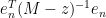
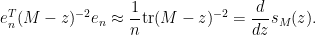
One can think of as a random (complex) Gaussian vector, divided by the magnitude of that vector (which, by the Chernoff inequality, will concentrate to ). Thus the coefficients with respect to the orthonormal basis can be thought of as independent (complex) Gaussian vectors, divided by that magnitude. Using this and the Chernoff inequality again, we see (for distance away from the real axis at least) that one has the concentration of measure

and thus

(that is to say, the diagonal entries of are roughly constant). Similarly we have

Inserting this into (5) and discarding terms of size , we thus conclude the approximate relationship

This can be viewed as a difference equation for the Stieltjes transform of top left minors of . Iterating this equation, and formally replacing the difference equation by a differential equation in the large limit, we see that when is large and for some , one expects the top left minor of to have Stieltjes transform

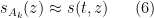
where solves the Burgers-type equation

with initial data .

Example 1 If is a constant multiple of the identity, then . One checks that is a steady state solution to (7), which is unsurprising given that all minors of are also times the identity.

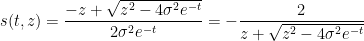
Example 2 If is GUE normalised so that each entry has variance , then by the semi-circular law (see previous notes) one has (using an appropriate branch of the square root). One can then verify the self-similar solution

to (7), which is consistent with the fact that a top minor of also has the law of GUE, with each entry having variance when .

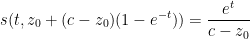
One can justify the approximation (6) given a sufficiently good well-posedness theory for the equation (7). We will not do so here, but will note that (as with the classical inviscid Burgers equation) the equation can be solved exactly (formally, at least) by the method of characteristics. For any initial position , we consider the characteristic flow formed by solving the ODE

with initial data , ignoring for this discussion the problems of existence and uniqueness. Then from the chain rule, the equation (7) implies that

and thus . Inserting this back into (8) we see that

and thus (7) may be solved implicitly via the equation

for all and .

Remark 3 In practice, the equation (9) may stop working when crosses the real axis, as (7) does not necessarily hold in this region. It is a cute exercise (ultimately coming from the Cauchy-Schwarz inequality) to show that this crossing always happens, for instance if has positive imaginary part then necessarily has negative or zero imaginary part.

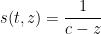
Example 4 Suppose we have as in Example 1. Then (9) becomes

for any , which after making the change of variables becomes

as in Example 1.

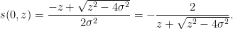
Example 5 Suppose we have

as in Example 2. Then (9) becomes

If we write

one can calculate that

and hence

which gives

One can recover the spectral measure from the Stieltjes transform as the weak limit of as ; we write this informally as

In this informal notation, we have for instance that

which can be interpreted as the fact that the Cauchy distributions converge weakly to the Dirac mass at as . Similarly, the spectral measure associated to (10) is the semicircular measure .

If we let be the spectral measure associated to , then the curve from to the space of measures is the high-dimensional limit of a Gelfand-Tsetlin pattern (discussed in this previous post), if the pattern is randomly generated amongst all matrices with spectrum asymptotic to as . For instance, if , then the curve is , corresponding to a pattern that is entirely filled with ‘s. If instead is a semicircular distribution, then the pattern is

thus at height from the top, the pattern is semicircular on the interval . The interlacing property of Gelfand-Tsetlin patterns translates to the claim that (resp. ) is non-decreasing (resp. non-increasing) in for any fixed . In principle one should be able to establish these monotonicity claims directly from the PDE (7) or from the implicit solution (9), but it was not clear to me how to do so.

An interesting example of such a limiting Gelfand-Tsetlin pattern occurs when , which corresponds to being , where is an orthogonal projection to a random -dimensional subspace of . Here we have

and so (9) in this case becomes

A tedious calculation then gives the solution

For , there are simple poles at , and the associated measure is

This reflects the interlacing property, which forces of the eigenvalues of the minor to be equal to (resp. ). For , the poles disappear and one just has

For , one has an inverse semicircle distribution

There is presumably a direct geometric explanation of this fact (basically describing the singular values of the product of two random orthogonal projections to half-dimensional subspaces of ), but I do not know of one off-hand.

The evolution of can also be understood using the -transform and -transform from free probability. Formally, letlet be the inverse of , thus

for all , and then define the -transform

The equation (9) may be rewritten as

and hence

or equivalently

See these previous notes for a discussion of free probability topics such as the -transform.

Example 6 If then the transform is .

Example 7 If is given by (10), then the transform is

Example 8 If is given by (11), then the transform is

This simple relationship (12) is essentially due to Nica and Speicher (thanks to Dima Shylakhtenko for this reference). It has the remarkable consequence that when is the reciprocal of a natural number , then is the free arithmetic mean of copies of , that is to say is the free convolution of copies of , pushed forward by the map . In terms of random matrices, this is asserting that the top minor of a random matrix has spectral measure approximately equal to that of an arithmetic mean of independent copies of , so that the process of taking top left minors is in some sense a continuous analogue of the process of taking freely independent arithmetic means. There ought to be a geometric proof of this assertion, but I do not know of one. In the limit (or ), the -transform becomes linear and the spectral measure becomes semicircular, which is of course consistent with the free central limit theorem.

In a similar vein, if one defines the function

and inverts it to obtain a function with

for all , then the -transform is defined by

Writing

for any , , we have

and so (9) becomes

which simplifies to

replacing by we obtain

and thus

and hence

One can compute to be the -transform of the measure ; from the link between -transforms and free products (see e.g. these notes of Guionnet), we conclude that is the free product of and . This is consistent with the random matrix theory interpretation, since is also the spectral measure of , where is the orthogonal projection to the span of the first basis elements, so in particular has spectral measure . If is unitarily invariant then (by a fundamental result of Voiculescu) it is asymptotically freely independent of , so the spectral measure of is asymptotically the free product of that of and of .

254A, Notes 5: Free probability

In the foundations of modern probability, as laid out by Kolmogorov, the basic objects of study are constructed in the following order:

1. Firstly, one selects a sample space , whose elements represent all the possible states that one’s stochastic system could be in.
2. Then, one selects a -algebra of events (modeled by subsets of ), and assigns each of these events a probability in a countably additive manner, so that the entire sample space has probability .
3. Finally, one builds (commutative) algebras of random variables (such as complex-valued random variables, modeled by measurable functions from to ), and (assuming suitable integrability or moment conditions) one can assign expectations to each such random variable.

In measure theory, the underlying measure space plays a prominent foundational role, with the measurable sets and measurable functions (the analogues of the events and the random variables) always being viewed as somehow being attached to that space. In probability theory, in contrast, it is the events and their probabilities that are viewed as being fundamental, with the sample space being abstracted away as much as possible, and with the random variables and expectations being viewed as derived concepts. See Notes 0 for further discussion of this philosophy.

However, it is possible to take the abstraction process one step further, and view the algebra of random variables and their expectations as being the foundational concept, and ignoring both the presence of the original sample space, the algebra of events, or the probability measure.

There are two reasons for wanting to shed (or abstract away) these previously foundational structures. Firstly, it allows one to more easily take certain types of limits, such as the large limit when considering random matrices, because quantities built from the algebra of random variables and their expectations, such as the normalised moments of random matrices tend to be quite stable in the large limit (as we have seen in previous notes), even as the sample space and event space varies with . (This theme of using abstraction to facilitate the taking of the large limit also shows up in the application of ergodic theory to combinatorics via the correspondence principle; see this previous blog post for further discussion.)

Secondly, this abstract formalism allows one to generalise the classical, commutative theory of probability to the more general theory of non-commutative probability theory, which does not have a classical underlying sample space or event space, but is instead built upon a (possibly) non-commutative algebra of random variables (or “observables”) and their expectations (or “traces”). This more general formalism not only encompasses classical probability, but also spectral theory (with matrices or operators taking the role of random variables, and the trace taking the role of expectation), random matrix theory (which can be viewed as a natural blend of classical probability and spectral theory), and quantum mechanics (with physical observables taking the role of random variables, and their expected value on a given quantum state being the expectation). It is also part of a more general “non-commutative way of thinking” (of which non-commutative geometry is the most prominent example), in which a space is understood primarily in terms of the ring or algebra of functions (or function-like objects, such as sections of bundles) placed on top of that space, and then the space itself is largely abstracted away in order to allow the algebraic structures to become less commutative. In short, the idea is to make algebra the foundation of the theory, as opposed to other possible choices of foundations such as sets, measures, categories, etc..

[Note that this foundational preference is to some extent a metamathematical one rather than a mathematical one; in many cases it is possible to rewrite the theory in a mathematically equivalent form so that some other mathematical structure becomes designated as the foundational one, much as probability theory can be equivalently formulated as the measure theory of probability measures. However, this does not negate the fact that a different choice of foundations can lead to a different way of thinking about the subject, and thus to ask a different set of questions and to discover a different set of proofs and solutions. Thus it is often of value to understand multiple foundational perspectives at once, to get a truly stereoscopic view of the subject.]

It turns out that non-commutative probability can be modeled using operator algebras such as -algebras, von Neumann algebras, or algebras of bounded operators on a Hilbert space, with the latter being accomplished via the Gelfand-Naimark-Segal construction. We will discuss some of these models here, but just as probability theory seeks to abstract away its measure-theoretic models, the philosophy of non-commutative probability is also to downplay these operator algebraic models once some foundational issues are settled.

When one generalises the set of structures in one’s theory, for instance from the commutative setting to the non-commutative setting, the notion of what it means for a structure to be “universal”, “free”, or “independent” can change. The most familiar example of this comes from group theory. If one restricts attention to the category of abelian groups, then the “freest” object one can generate from two generators is the free abelian group of commutative words with , which is isomorphic to the group . If however one generalises to the non-commutative setting of arbitrary groups, then the “freest” object that can now be generated from two generators is the free group of non-commutative words with , which is a significantly larger extension of the free abelian group .

Similarly, when generalising classical probability theory to non-commutative probability theory, the notion of what it means for two or more random variables to be independent changes. In the classical (commutative) setting, two (bounded, real-valued) random variables are independent if one has

whenever are well-behaved functions (such as polynomials) such that , both vanish. In the non-commutative setting, one can generalise the above definition to two commuting bounded self-adjoint variables; this concept is useful for instance in quantum probability, which is an abstraction of the theory of observables in quantum mechanics. But for two (bounded, self-adjoint) non-commutative random variables , the notion of classical independence no longer applies. As a substitute, one can instead consider the notion of being freely independent (or free for short), which means that

whenever are well-behaved functions such that all of vanish.

The concept of free independence was introduced by Voiculescu, and its study is now known as the subject of free probability. We will not attempt a systematic survey of this subject here; for this, we refer the reader to the surveys of Speicher and of Biane. Instead, we shall just discuss a small number of topics in this area to give the flavour of the subject only.

The significance of free probability to random matrix theory lies in the fundamental observation that random matrices which are independent in the classical sense, also tend to be independent in the free probability sense, in the large limit . (This is only possible because of the highly non-commutative nature of these matrices; as we shall see, it is not possible for non-trivial commuting independent random variables to be freely independent.) Because of this, many tedious computations in random matrix theory, particularly those of an algebraic or enumerative combinatorial nature, can be done more quickly and systematically by using the framework of free probability, which by design is optimised for algebraic tasks rather than analytical ones.

Much as free groups are in some sense “maximally non-commutative”, freely independent random variables are about as far from being commuting as possible. For instance, if are freely independent and of expectation zero, then vanishes, but instead factors as . As a consequence, the behaviour of freely independent random variables can be quite different from the behaviour of their classically independent commuting counterparts. Nevertheless there is a remarkably strong analogy between the two types of independence, in that results which are true in the classically independent case often have an interesting analogue in the freely independent setting. For instance, the central limit theorem (Notes 2) for averages of classically independent random variables, which roughly speaking asserts that such averages become gaussian in the large limit, has an analogue for averages of freely independent variables, the free central limit theorem, which roughly speaking asserts that such averages become semicircular in the large limit. One can then use this theorem to provide yet another proof of Wigner’s semicircle law (Notes 4).

Another important (and closely related) analogy is that while the distribution of sums of independent commutative random variables can be quickly computed via the characteristic function (i.e. the Fourier transform of the distribution), the distribution of sums of freely independent non-commutative random variables can be quickly computed using the Stieltjes transform instead (or with closely related objects, such as the -transform of Voiculescu). This is strongly reminiscent of the appearance of the Stieltjes transform in random matrix theory, and indeed we will see many parallels between the use of the Stieltjes transform here and in Notes 4.

As mentioned earlier, free probability is an excellent tool for computing various expressions of interest in random matrix theory, such as asymptotic values of normalised moments in the large limit . Nevertheless, as it only covers the asymptotic regime in which is sent to infinity while holding all other parameters fixed, there are some aspects of random matrix theory to which the tools of free probability are not sufficient by themselves to resolve (although it can be possible to combine free probability theory with other tools to then answer these questions). For instance, questions regarding the rate of convergence of normalised moments as are not directly answered by free probability, though if free probability is combined with tools such as concentration of measure (Notes 1) then such rate information can often be recovered. For similar reasons, free probability lets one understand the behaviour of moments as for fixed , but has more difficulty dealing with the situation in which is allowed to grow slowly in (e.g. ). Because of this, free probability methods are effective at controlling the bulk of the spectrum of a random matrix, but have more difficulty with the edges of that spectrum (as well as with related concepts such as the operator norm, Notes 3) as well as with fine-scale structure of the spectrum. Finally, free probability methods are most effective when dealing with matrices that are Hermitian with bounded operator norm, largely because the spectral theory of bounded self-adjoint operators in the infinite-dimensional setting of the large limit is non-pathological. (This is ultimately due to the stable nature of eigenvalues in the self-adjoint setting; see this previous blog post for discussion.) For non-self-adjoint operators, free probability needs to be augmented with additional tools, most notably by bounds on least singular values, in order to recover the required stability for the various spectral data of random matrices to behave continuously with respect to the large limit. We will discuss this latter point in a later set of notes.