
Let 


of 

A basic question in linear algebra asks the extent to which the eigenvalues 


when expressed in terms of eigenvalues, gives the trace constraint


(together with the counterparts for 


and so forth.
The complete answer to this problem is a fascinating one, requiring a strangely recursive description (once known as Horn’s conjecture, which is now solved), and connected to a large number of other fields of mathematics, such as geometric invariant theory, intersection theory, and the combinatorics of a certain gadget known as a “honeycomb”. See for instance my survey with Allen Knutson on this topic some years ago.
In typical applications to random matrices, one of the matrices (say, 

valid whenever 


One consequence of these inequalities is that the spectrum of a Hermitian matrix is stable with respect to small perturbations.
We will also establish some closely related inequalities concerning the relationships between the eigenvalues of a matrix, and the eigenvalues of its minors.
Many of the inequalities here have analogues for the singular values of non-Hermitian matrices (which is consistent with the discussion near Exercise 16 of Notes 3). However, the situation is markedly different when dealing with eigenvalues of non-Hermitian matrices; here, the spectrum can be far more unstable, if pseudospectrum is present. Because of this, the theory of the eigenvalues of a random non-Hermitian matrix requires an additional ingredient, namely upper bounds on the prevalence of pseudospectrum, which after recentering the matrix is basically equivalent to establishing lower bounds on least singular values. We will discuss this point in more detail in later notes.
We will work primarily here with Hermitian matrices, which can be viewed as self-adjoint transformations on complex vector spaces such as 

— 1. Proof of spectral theorem —
To prove the spectral theorem, it is convenient to work more abstractly, in the context of self-adjoint operators on finite-dimensional Hilbert spaces:
Theorem 1 (Spectral theorem) Let
be a finite-dimensional complex Hilbert space of some dimension
be a self-adjoint operator. Then there exists an orthonormal basis
of
such that
for all
.
The spectral theorem as stated in the introduction then follows by specialising to the case 
Proof: We induct on the dimension 


Let 


this simplifies using self-adjointness to

Since 


Suppose we have a self-adjoint transformation 


Exercise 1 Suppose that the eigenvalues
of an
is unique up to rotating each individual eigenvector
by a complex phase
. In particular, the spectral projections
are unique. What happens when there is eigenvalue multiplicity?
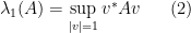
— 2. Minimax formulae —
The 


Theorem 2 (Courant-Fischer min-max theorem) Let
for all


Proof: It suffices to prove (6), as (7) follows by replacing 

We first verify the

whenever 
To prove the general case, we may again assume 

so we only need to prove the reverse inequality. In other words, for every 

Let 


Remark 1 By homogeneity, one can replace the restriction
with
provided that one replaces the quadratic form
with the Rayleigh quotient
.
A closely related formula is as follows. Given an 


where 
Proposition 3 (Extremal partial trace) Let
, one has
and


As a corollary, we see that 

Proof: Again, by symmetry it suffices to prove the first formula. As before, we may assume without loss of generality that 

so it suffices to prove the reverse inequality. For this we induct on dimension. If 


On the other hand, if

Adding the two inequalities we obtain the claim.
Specialising Proposition 3 to the case when


for any 
Exercise 2 Show that the inequalities (9) are equivalent to the assertion that the diagonal entries
lies in the permutahedron of
permutations of
in
Remark 2 It is a theorem of Schur and Horn that these are the complete set of inequalities connecting the diagonal entries
of a matrix
under the diagonal map
is the permutahedron of
as the moment map associated with the conjugation action of the standard maximal torus of
(i.e. the diagonal unitary matrices) on the coadjoint orbit. When viewed in this fashion, the Schur-Horn theorem can be viewed as the special case of the more general Atiyah convexity theorem (also proven independently by Guillemin and Sternberg) in symplectic geometry. Indeed, the topic of eigenvalues of Hermitian matrices turns out to be quite profitably viewed as a question in symplectic geometry (and also in algebraic geometry, particularly when viewed through the machinery of geometric invariant theory).
There is a simultaneous generalisation of Theorem 2 and Proposition 3:
Exercise 3 (Wielandt minimax formula) Let
of subspaces of
for all
. Define the associated Schubert variety
to be the collection of all
. Show that for any

— 3. Eigenvalue inequalities —
Using the above minimax formulae, we can now quickly prove a variety of eigenvalue inequalities. The basic idea is to exploit the linearity relationship

for any unit vector

for any subspace
For instance, as mentioned before, the inequality (3) follows immediately from (2) and (10). Similarly, for the Ky Fan inequality (5), one observes from (11) and Proposition 3 that

for any


for any
In a similar spirit, using the inequality

for unit vectors

thus the spectrum of
More generally, suppose one wants to establish the Weyl inequality (4). From (6) that it suffices to show that every 

But from (6), one can find a subspace 


Remark 3 More generally, one can generate an eigenvalue inequality whenever the intersection numbers of three Schubert varieties of compatible dimensions is non-zero; see the paper of Helmke and Rosenthal. In fact, this generates a complete set of inequalities; this is a result of Klyachko. One can in fact restrict attention to those varieties whose intersection number is exactly one; this is a result of Knutson, Woodward, and myself. Finally, in those cases, the fact that the intersection is one can be proven by entirely elementary means (based on the standard inequalities relating the dimension of two subspaces
to their intersection
); this is a result of Bercovici, Collins, Dykema, Li, and Timotin. As a consequence, the methods in this section can, in principle, be used to derive all possible eigenvalue inequalities for sums of Hermitian matrices.
Exercise 4 Verify the inequalities (12) and (4) by hand in the case when
Exercise 5 Establish the dual Lidskii inequality
for any
whenever
.


Exercise 6 Use the Lidskii inequality to establish the more general inequality
whenever
, and
is the decreasing rearrangement of
. (Hint: express
as the integral of
as
runs from
to infinity. For each fixed
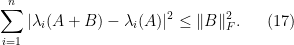
-Weilandt-Hoffman inequality
for any
, where
is the usual
norm (with the usual convention that
), and
is the


Exercise 7 Show that the
Exercise 8 Show that for any
, one has

Exercise 9 Establish the Hölder inequality
whenever
with
, and

The most important 


where 


We will give an alternate proof of this inequality, based on eigenvalue deformation, in the next section.
— 4. Eigenvalue deformation —
From the Weyl inequality (13), we know that the eigenvalue maps
Exercise 10 (Dimension count) Suppose that
. Show that the space of Hermitian matrices with at least one repeated eigenvalue has codimension
in the space of all Hermitian matrices, and the space of real symmetric matrices with at least one repeated eigenvalue has codimension
Let us say that a Hermitian matrix has simple spectrum if it has no repeated eigenvalues. We thus see from the above exercise and (13) that the set of Hermitian matrices with simple spectrum forms an open dense set in the space of all Hermitian matrices, and similarly for real symmetric matrices; thus simple spectrum is the generic behaviour of such matrices. Indeed, the unexpectedly high codimension of the non-simple matrices (naively, one would expect a codimension 

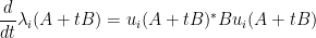
We first observe that when 


Now suppose that 


to obtain various equations of motion for 

Let’s see how this works. Taking first derivatives of (18), (19) using the product rule, we obtain

The equation (21) simplifies to 


This can already be used to give alternate proofs of various eigenvalue identities. For instance, If we apply this to 
whenever 


Exercise 11 Use a similar argument to the one above to establish (17) without using minimax formulae or Lidskii’s inequality.
Exercise 12 Use a similar argument to the one above to deduce Lidskii’s inequality (12) from Proposition 3 rather than Exercise 3.
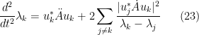
One can also compute the second derivative of eigenvalues:
Exercise 13 Suppose that
whenever
If one interprets the second derivative of the eigenvalues as being proportional to a “force” on those eigenvalues (in analogy with Newton’s second law), (23) is asserting that each eigenvalue
“repels” the other eigenvalues
by exerting a force that is inversely proportional to their separation (and also proportional to the square of the matrix coefficient of
in the eigenbasis). See this earlier blog post for more discussion.
Remark 4 In the proof of the four moment theorem of Van Vu and myself, which we will discuss in a subsequent lecture, we will also need the variation formulae for the third, fourth, and fifth derivatives of the eigenvalues (the first four derivatives match up with the four moments mentioned in the theorem, and the fifth derivative is needed to control error terms). Fortunately, we do not need the precise formulae for these derivatives (which, as one can imagine, are quite complicated), but only their general form, and in particular an upper bound for these derivatives in terms of more easily computable quantities.
— 5. Minors —
In the previous sections, we perturbed 


Exercise 14 (Cauchy interlacing inequalities) For any
for all

Remark 5 If one takes successive minors
of an
One can obtain a more precise formula for the eigenvalues of
Exercise 15 (Eigenvalue equation) Let
where
is the bottom right entry of
is the right column of
into the
and
components.) Note the similarities between (25) and (23).
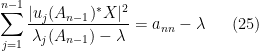
Observe that the function 

The identity (25) suggests that under typical circumstances, an eigenvalue 

— 6. Singular values —
The theory of eigenvalues of 
Theorem 4 (Singular value decomposition) Let
, and let
.) Then there exist non-negative real numbers
(known as the singular values of
and
(known as singular vectors of
for all
, where we abbreviate
, etc.
Furthermore,
whenever
is orthogonal to all of the
.


We adopt the convention that 

Proof: We induct on 


We follow a similar strategy to the proof of Theorem 1. We may assume that 


Exercise 16 Show that the singular values
of a
, show that the singular vectors are unique up to rotation by a complex phase.
By construction (and the above uniqueness claim) we see that 

Exercise 17 If
, show that the augmented matrix
is a
Hermitian matrix whose eigenvalues consist of
, together with
copies of the eigenvalue zero. (This generalises Exercise 16 from Notes 3.) What is the relationship between the singular vectors of
?

Exercise 18 If
of
of
Remark 6 When
Exercise 19 If
has eigenvalues
, and
has eigenvalues
Exercise 20 Show that the rank of a
Exercise 21 Let
for all
, where the supremum ranges over all subspaces of

One can use the above exercises to deduce many inequalities about singular values from analogous ones about eigenvalues. We give some examples below.
Exercise 22 Let
- (i) Establish the Weyl inequality
whenever
.
- (ii) Establish the Lidskii inequality
whenever
.
- (iii) Show that for any
, the map
defines a norm on the space
of complex
Ky Fan norm).
- (iv) Establish the Weyl inequality
for all
- (v) More generally, establish the
-Weilandt-Hoffman inequality
for any
, where
is the
- (vi) Show that the
- (vii) If
is formed by removing one row from
for all
.
- (viii) If
and
. What changes when
?


Exercise 23 Let
naturally induces a linear transformation
from
the structure of a Hilbert space by declaring the basic forms
for
For any
is equal to
.
Exercise 24 Let
matrix, and let
matrix for some
.
Show that
and
for any
Exercise 25 Let
be a
be distinct, and let
be distinct. Show that
Using this, show that if
are distinct, then
for every


Exercise 26 Establish the Hölder inequality
whenever
are such that
.
Acknowledgments: Thanks to Allen Knutson for corrections.

70 comments
Comments feed for this article
13 January, 2010 at 6:10 am
Marius
Hi Terry,
Linear algebra is indeed fascinating. Maybe the readers of this post may find
interesting some connections between this subject and quasiconvexity in the
calculus of variations and nonlinear elasticity:
http://www.sciencedirect.com/science?_ob=ArticleURL&_udi=B6V0R-4SPSHN6-3&_user=3797462&_rdoc=1&_fmt=&_orig=search&_sort=d&_docanchor=&view=c&_searchStrId=1164865628&_rerunOrigin=google&_acct=C000061416&_version=1&_urlVersion=0&_userid=3797462&md5=d8361adf4dc60e9323fc42216695b1cd
or
Click to access major_stem.pdf
14 January, 2010 at 1:50 pm
Anonymous
A potential typo: in eq. 19 (and elsewhere), I thought the norm should be 1, not 0.
[Corrected, thanks – T.]
15 January, 2010 at 7:59 am
kashif
A small typo start of section 4: “From the Weyl inequality (13) we now that…” should be “From the Weyl inequality (13) we know that…”
[Corrected, thanks – T.]
18 January, 2010 at 6:29 pm
254A, Notes 3b: Brownian motion and Dyson Brownian motion « What’s new
[…] from the first and second Hadamard variation formulae (see Section 4 of Notes 3a) we […]
19 January, 2010 at 4:15 pm
David Speyer
Possible typo: Should equation (19) read u_i^* u_i =1 (rather than 0)?
[Ack, I thought I corrected that typo already. Corrected again, thanks – T.]
2 February, 2010 at 1:34 pm
254A, Notes 4: The semi-circular law « What’s new
[…] first observation is that the Cauchy interlacing law (Exercise 14 from Notes 3a) shows that the ESD of is very stable in . Indeed, we see from the interlacing law […]
17 February, 2010 at 8:30 am
Steven Heilman
Some pretty pedantic potential corrections:
1. A basic question in linear algebra …\lambda_{1}(B),\ldots,\lambda_{n}(B)
2. Eqs. (5),(9),(12): numerical label outside viewing window?
3. Section 3: Similarly, [for] the Ky Fan…
4. Section 4: From the Weyl inequality… we [k]now
5. After Exercise 10: … from the above exercise and [ ] (13)
6(a). Statement of Theorem 4: A^* v_j=\sigma_j u_j
6(b). Proof of Theorem 4: \sigma_1 :=\|Au_1 \|>0 ?
7. Exercise 23: induces a linear transformation … \bigwedge^k {\mathbb C}^p …
——————-
[and a few for Notes 3b]
1. After Remark 6: Applying [Lemma] (5)
2. … with disjoint increments being jointly indepen[d]ent
3. Proof of Theorem 6: …G continues [to] have the GUE distribution…
[Corrected, thanks – T.]
23 February, 2010 at 10:02 pm
254A, Notes 6: Gaussian ensembles « What’s new
[…] is simple. Since almost all Hermitian matrices have simple spectrum (see Exercise 10 of Notes 3a), this gives the full spectral distribution of GUE, except for the issue of the unspecified […]
14 March, 2010 at 11:33 am
254A, Notes 8: The circular law « What’s new
[…] case, where eigenvalue inequalities such as the Weyl inequalities or Hoffman-Wielandt inequalities (Notes 3a) ensure stability of the […]
8 May, 2010 at 1:30 am
Anonymous
Dear Prof. Tao,
I had some problems on Ex. 8 and Ex. 13:
Ex. 8: Could you give some hint on how to prove it? This is most probably very trivial, but I tried it for several hours.
Ex. 13: I tried to do it according to your hint, but it is hard for me how to make the other eigenvalues involved in the equations of
  .
.
Thank you very much in advance!
8 May, 2010 at 1:12 pm
Terence Tao
For Ex 8, apply the method of Ex6 but with (12) replaced by (9).
For Ex13, a solution can be found at the link provided.
21 May, 2010 at 10:11 am
Ben
Hi, in a neighbourhood of
  . Is there not an issue that the matrix
  is singular? Is this where the normalization
  comes in? Thanks for your help.
I’m a bit confused about your use of the inverse/implicit function theorem to get smoothness of the eigenvectors
21 May, 2010 at 12:07 pm
Terence Tao
Yes, with the normalisation (and working in the real symmetric setting for simplicity), the map
  is a map from an n-dimensional space
  to an n-dimensoinal space
  , and one can check by hand that the Jacobian is nondegenerate when the eigenvalues are simple, so the inverse theorem lets one select both
  and
and  smoothly in this case. In the complex Hermitian setting it is a bit more complicated, one has to also fix the phase of one of the coordinates of
  (e.g. insisting that the first coordinate is a positive real) to make the dimensions match.
There is a theorem of Rellich that shows that eigenvectors and eigenvalues can in fact be selected in an analytic fashion even when there are repeated eigenvalues, but only if one abandons the idea of keeping the order of the eigenvalues fixed (i.e. one allows one eigenvalue to overtake another). This is a nontrivial theorem to prove, though.
2 October, 2014 at 10:02 am
hmobahi
Thank you Terrence. This was an extremely helpful comment. Does your comment imply that the function \sum_{k=1}^n (\frac{d}{d t} \lambda_k(t)) f_k(\lambda_k(t)) is well-defined even when eigenvalues are not simple? Here f_k(x) is any functional that analytically depends on x. I think about this, because the sum kills the dependency of a specific ordering of the eigenvaules.
30 May, 2010 at 5:12 pm
Anonymous
Question and a correction.
In Exercise 5, the second inequality should be A->A+B
n->A, n->B.
Question: could a hint be given on how to prove the p-Weilandt-Hoffman inequality using Holder’s inequality? I do not have any clue.
30 May, 2010 at 11:05 pm
Terence Tao
Thanks for the correction!
By Holder’s inequality, the norm of a sequence is equal to the largest inner product between that sequence and a sequence of unit
  norm. Now use the fact that the
  norm is invariant with respect to rearrangement.
6 February, 2012 at 9:03 pm
Anonymous
Dear Prof. Tao, to get to get the first inequality in Exercise 6, do you multiply the Lidskii’s inequality by the integral given in the hint, and then how can one get or have an rearrangement of
  in front of
  ? Thanks for your help!
31 May, 2010 at 11:48 am
Anonymous
Thanks for the reply. But I am still confused about how to get (14) using ONLY the first inequality given in Exercise 6 and the Holder’s inequality.
TO generate the l_p norm for (\lamda_{i}(A+B)-\lamda_{i}(A)) using Holder’s inequality, we need to use a c_i that is negative if (\lamda_{i}(A+B)-\lamda_{i}(A)) is negative.
But this inequality is only about c_i that is nonnegative.
For example, consider the scalar case when A,B are both scalars, \lamda_{1}(A+B)-\lamda_{1}(A) <\lamda_1(B), does not necessarily mean the absolute value of the former is smaller than the absolute value of the latter.
Should we use some other conditions?
31 May, 2010 at 6:56 pm
Terence Tao
Because the trace of A+B is the sum of the trace of A and the trace of B, one can extend the original inequality to the case when the c_i are arbitrary reals.
6 February, 2012 at 9:06 pm
Anonymous
Dear Prof. Tao, to get the first inequality in Exercise 6, do you multiply the Lidskii’s inequality by the integral given in the hint, and then how can one get or have an rearrangement of
  in front of
  ? Thanks for your help!
22 December, 2010 at 9:08 pm
Outliers in the spectrum of iid matrices with bounded rank permutations « What’s new
[…] were no interlacing inequalities in this case to control bounded rank perturbations (as discussed in this post). However, as it turns out I had arrived at the wrong conclusion, especially in the exterior of the […]
19 January, 2011 at 6:55 pm
San
In proposition3, how do you use induction hypothesis, as the hypothesis would be true for the sum of first k eigenvalues.
Thanks,
San
20 January, 2011 at 12:13 pm
Terence Tao
When one restricts A to the span of to obtain an n-1-dimensional linear operator, the eigenvalues are now
  , thanks to the hypothesis that A has the standard eigenbasis (so that it is given by the diagonal matrix with entries
  .
.
20 January, 2011 at 5:41 pm
San
Thanks for the reply. Can I ask where can I find the solution of exercise3.
Sangeeta
24 July, 2019 at 5:37 am
Anonymous
https://math.stackexchange.com/q/2863568/469791
22 January, 2011 at 9:26 am
Sandor
A direct link to “my survey with Allen Knutson” is http://www.ams.org/notices/200102/fea-knutson.pdf
22 August, 2011 at 4:17 am
Interlaced eigenvalues « Alasdair's musings
[…] Another proof uses the min-max theorem, of which a full account is given by Terry Tao. […]
13 February, 2012 at 8:52 am
kushal
Hi,
1.Is there any upper bound for the norm of the inverse of a matrix (i.e. ||inv(A)||), in terms of the norm of the matrix , i.e. ||A|| ?
NB. There is no restriction on A such as det(A)= ???
Is there any lower bound for problem-2 that involves only A and not inv(A)?
11 July, 2013 at 11:03 am
Anonymous
Hello Prof. Tao,
Can these results be applied to matrices of differnt dimensions? For example, I have a m*m matrix (A) of rank n<m, and add another matrix of dimension q*q (B), where q< n. All matrices are Hermitian. Can I find a bound on the absolute eigenvalues of the system? The eigenvalues are lambda_1, – lambda_1, lambda_2, -lambda_2, and so on.
16 April, 2014 at 3:42 pm
Anonymous
Is there a relation for the eigenvalues of the sum of an anti-Hermitian A and a Hermitian matrix B? For example, if I want to know the eigenvalues of A + B, can I simply calculate the eigenvalues of A and B seperately and then get the eigenvalues of A + B from them?
16 April, 2014 at 4:03 pm
Terence Tao
If A and B commute, then the eigenvalues of A+B are the sum of eigenvalues of A and some permutation of the eigenvalues of B.
In general, though, the situation is quite complicated, since A+B will usually not be a normal matrix, and the eigenvalues will be quite badly behaved complex numbers. One can still control the singular values, and hence the eigenvalues to some extent, by the Weyl inequalities, and one also controls the trace of A+B, but other than that things look quite messy, even for the 2×2 matrix case.
26 August, 2015 at 4:38 am
Hamed
I do not know about the application you have in mind. But in case you need to know the bounds of eigenvalues (for example if you want to analysis the stability of some dynamical system) this structure can help you. You can use Bendixon’s theorem which says that the eigenvalues of A+B are bounded in a box, when the real parts are bounded by eigenvalues of B (Hermitian) and the imaginary parts are bounded by eigenvalues of A (anti-Hermitian).
27 June, 2014 at 2:18 am
Felix V.
Dear Professor Tao,
in Exercise 10, you ask the reader to proof that
“the space of Hermitian matrices with at least one repeated eigenvalue has codimension {3} in the space of all Hermitian matrices.”
It seemed to me that “space” should be interpreted as “(real) vector space” in this context.
But then the problem is that the set of matrices with at least one repeated eigenvalue is NOT a vector space (not closed under addition), as can be seen by considering e.g. diagonal matrices:
{
\left(\begin{array}{ccc}
1\\
& 1\\
& & 2
\end{array}\right)+\left(\begin{array}{ccc}
0\\
& 1\\
& & 1
\end{array}\right)=\left(\begin{array}{ccc}
1\\
& 2\\
& & 3
\end{array}\right)
}
Best regards,
Felix V.
27 June, 2014 at 8:10 am
Terence Tao
Here I am not interpreting “space” in the linear algebra sense; you may substitute “set” or “algebraic set” instead, if you prefer.
17 March, 2015 at 5:47 am
Lecture #22: Random Sampling for Fast SVDs | CMU Advanced Algos: S15
[…] pointed out that it follows from the Weyl inequalities. These say that for all integers such that […]
28 March, 2015 at 7:57 pm
kumar vishwajeet
Dear Dr Tao, be a random complex matrix of size
  .
.  has circular Gaussian distribution with mean 0 and variance
 where
where  has Gaussian distribution with mean 0 and variance
  . Using monte Carlo, I found that the probaility density function of the
  and that of
  only differs by a multiplying constant. Is there any mathematical proof or logical explanation for this?
I am currently working on the distribution of eigenvalues of non central wishart matrices. I found the following interesting thing.
Let
Consider another case where,
29 March, 2015 at 8:08 am
Terence Tao
The eigenvalues of and
and  are the squares of the eigenvalues of the Hermitian matrices
  and
and 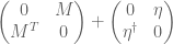 respectively. So my guess is that the matrices
  and
and  have essentially the same spectrum (semicircle law, I think) and are behaving as if they were free of
  . (I’m not sure what you mean by the multiplying constant difference though – the probability density function has to integrate to 1.)
28 March, 2015 at 8:12 pm
kumar vishwajeet
Just a modification of my last post: The probability density function of eigenvalues of and
and  differ by a multiplying constant.
29 March, 2015 at 12:46 pm
kumar vishwajeet
Thank you for the prompt reply. be the pdf of eigenvalues of
  and
and  be the pdf of eigenvalues of
  , then
By “Multiplying constant difference” I mean that if
29 March, 2015 at 3:12 pm
kumar vishwajeet
I got it. has to be equal to one.
24 September, 2015 at 4:31 pm
Abbas
What does $|Av|$ denote in Exercise 21?
[The magnitude of the vector formed by multiplying the matrix
  with the vector
  . -T.]
30 March, 2016 at 4:39 pm
David
Prof. Tao,
I am a novice going through a few of these exercises and ran into trouble on #6. Here you suggest using Holder’s inequality to prove the p-Wielandt Hoffman inequality. This works very straightforwardly to yield an Lp norm for the right hand side of the inequality (in (14)), but the Lp norm also must be obtained on the left hand side, which is more difficult. Can you comment on how to proceed for the left hand side of (14)?
30 March, 2016 at 9:24 pm
Terence Tao
Use the converse form of Holder’s inequality.
31 March, 2016 at 11:22 am
David
Very nice, thanks.
24 May, 2016 at 4:44 am
Anonymous
Dear Dr. Tao,
I was thinking about a way to show that the partial trace is independent of the choice an orthonormal basis. But I kept failing to find a good proof. Is there any hint you can give me ?
24 May, 2016 at 8:35 am
Terence Tao
Given two orthonormal bases for , write the elements of one basis as a linear combination of the other basis; the coefficients will then form a unitary matrix since both bases are orthonormal. Insert these expansions of the basis elements to write the partial trace in one basis in terms of the other basis, and use the definition of a unitary matrix to simplify.
Alternatively, one can note that the partial trace is also equal to the full trace of , where
  is the orthogonal projection onto
  , and use the standard fact that the full trace is basis-independent.
24 May, 2016 at 10:32 am
Anonymous
Thank you, the second one is the one I was looking for.
27 May, 2016 at 12:01 am
David
Dear Dr. Tao,
I would be interested to see the proof of the dual Weyl inequality if you happen to have it handy. I have read the proof in “A Note on Weyl’s Inequality” by Steve Fisk, but I failed to really understand it.
Thanks,
David
27 May, 2016 at 7:56 am
Terence Tao
One can for instance derive the dual Weyl inequality from the original Weyl inequality by repeatedly using the identity .
.
24 June, 2016 at 8:43 am
vsk1996
Tao sir please give some simpler version of (Courant-Fischer Theorem) and relate it with rayleigh quotient
25 October, 2016 at 3:39 am
Archy
Prof. Tao, is there a simplification of this theory, if all the Hermitian matrices are rank 1? thank you very much!
26 November, 2016 at 11:05 am
keej
These notes are great. I think there is a typo in the definition of spectral projection in Exercise 1. It should be $u_j(A) u_j(A)^*$, not $u_j(A)^* u_j(A)$.
[Corrected, thanks – T.]
2 March, 2017 at 12:08 am
keej
In the proof of the SVD, we use the fact that a critical point of the map must satisfy the identity
  . I have two questions about this.
First, I can see why this is true by expanding out all the entries and differentiating, but I feel like there should be a faster way. Is there?
Secondly, what does the derivative even mean in the case that has complex entries? The map in question is real-valued, so how can its gradient be a complex vector?
2 March, 2017 at 9:48 am
Terence Tao
One can first try to understand the situation when is a diagonal matrix, in which case the map basically splits as the sum of
  non-interacting one-dimensional maps, and the claim is then easy to understand in that setting. The existence of the SVD in fact tells us that the critical point behaviour of a general matrix
  will be the same as that of a diagonal matrix (with the singular values as entries), so if one believes the SVD to exist then this explains why this identity ought to be true. Of course one cannot use this observation to prove the existence of SVD, as this would be circular, but it can certainly be used to motivate such a proof.
Any complex vector space can be viewed as a real vector space of twice the dimension, so one can take the gradient in that setting.
16 February, 2018 at 4:52 pm
Dita
Dear Prof. Tao, I have one question. If the eigenvalues of matrices A and
A + B are increasing ordered, but the eigenvalues of B are not ordered, is it possible to use Weyl’s inequality to get a bound for the eigenvalue of A + B? Thank you for your attention.
4 May, 2018 at 10:55 am
Anonymous
Is the Weyl’s inequality true even in the case when we have separable Hilbert space?
4 May, 2018 at 12:54 pm
Terence Tao
For compact self-adjoint operators, basically all the inequalities for finite-dimensional operators extend to the infinite-dimensional setting by a limiting argument, see https://arxiv.org/abs/0709.1088 . For non-compact operators, in which the spectrum need not be pure point, the situation is significantly more complicated, and I am not sure what can cleanly be said (beyond the subadditivity of operator norms).
12 July, 2018 at 4:08 pm
Anonymous
Do (vii/viii) in Exercise 22 imply that cauchy interlacing theorem holds for eigenvalues of matrices that not necessarily hermitian?
[Oops, this was a typo: all references to eigenvalues here have been replaced with singular values. There is no interlacing for eigenvalues for non-Hermitian matrices, as these eigenvalues need not even be real. -T.]
6 April, 2019 at 5:48 pm
Schur-Horn | Random Mathematics
[…] do: Do the exercises of this post by […]
7 April, 2019 at 5:27 am
Diagonalization of Hermitian matrices | Random Mathematics
[…] Following Tao’s post here. […]
7 April, 2019 at 7:48 am
Courant-Fischer min-max Theorem | Random Mathematics
[…] Following Tao’s post here. […]
7 April, 2019 at 1:16 pm
Extremal partial traces | Random Mathematics
[…] Following Tao’s post. […]
7 April, 2019 at 6:07 pm
Wielandt minimax formula | Random Mathematics
[…] This is exercise 3 in Tao’s post here. […]
30 April, 2020 at 4:49 pm
Hamiltonian Density of States – Ramis Movassagh
[…] Horn’s conjecture was finally proved by Alexander Klaychko in (1998). Later Knutson and Tao gave a proof based on Honey comb puzzles and Schubert calculus (see this post). […]
30 September, 2020 at 10:02 am
Vaibhav
Does the positive-definiteness of the matrices A and B alter the eigenvalue inequalities, such as, Weyl inequalities? Is that a condition that needs consideration? Thanks in advance!
1 October, 2020 at 7:54 am
Terence Tao
Any self-adjoint matrix can be made positive definite by adding a large multiple of the identity, which has the effect of translating all the eigenvalues by a constant. One can check that inequalities such as Weyl’s inequalities are invariant under such a translation, hence the imposition of positive definiteness does not lead to any significant improvement to Weyl’s inequalities. On the other hand, being positive definite is equivalent to the eigenvalues being non-negative, so one now has some additional inequalities that one can combine with Weyl’s inequalities if one wishes to obtain some new, but *weaker* inequalities. For instance by adding
  to
to  one gets the new, but worse, inequality
  .
.
18 March, 2021 at 12:17 pm
The Better Way to Convert an SVD into a Symmetric Eigenvalue Problem – Ethan Epperly
[…] This approach of using the Hermitian dilation to compute the SVD of fixes all the issues identified with the “” approach. We are able to accurately resolve a full 16 orders of magnitude of singular values. The computed singular vectors are accurate and numerically orthogonal provided we use an accurate method for the symmetric eigenvalue problem. The Hermitian dilation preserves important structural characteristics in like sparsity. For purposes of theoretical analysis, the mapping is linear.5The linearity of the Hermitian dilation gives direct extensions of most results about the symmetric eigenvalues to singular values; see Exercise 22. […]
1 January, 2022 at 2:08 pm
Xavier Mootoo
Thank you Dr. Tao, this was really helpful for understanding the Courant-Fischer Theorem!
4 July, 2022 at 11:20 pm
matrices - Is there relation between eigenvalues of A,B,A+B,AB? Answer - Lord Web
[…] I found there are some works about eigenvalues of $A,B,A+B$ in the case of Hermitian matrices. For example, here. […]
30 January, 2024 at 8:45 pm
Anonymous
Hi professor,
Regarding the proof of the Hadamard first variation formula I am unable to see why for Hermitian matrices $\dot{u}_i^*u_i = 0$. If the inner product or eigenvectors were real this would be immediate from differentiating the unit norm condition, but for the complex inner product I only see that the real part must vanish. How can one show that the imaginary part vanishes as well?
[Real part inserted into the claim; control of the imaginary part is not needed for the rest of the argument. -T]