245A, Notes 1: Lebesgue measure

9 September, 2010 in 245A - Real analysis, math.CA | Tags: axiom of choice, Lebesgue measure, outer measure | by Terence Tao

In the prologue for this course, we recalled the classical theory of Jordan measure on Euclidean spaces ${{\bf R}^d}$ . This theory proceeded in the following stages:

First, one defined the notion of a box ${B}$ and its volume ${|B|}$ .
Using this, one defined the notion of an elementary set ${E}$ (a finite union of boxes), and defines the elementary measure ${m(E)}$ of such sets.
From this, one defined the inner and outer Jordan measures ${m_{*,(J)}(E), m^{*,(J)}(E)}$ of an arbitrary bounded set ${E \subset {\bf R}^d}$ . If those measures match, we say that ${E}$ is Jordan measurable, and call ${m(E) = m_{*,(J)}(E) = m^{*,(J)}(E)}$ the Jordan measure of ${E}$ .

As long as one is lucky enough to only have to deal with Jordan measurable sets, the theory of Jordan measure works well enough. However, as noted previously, not all sets are Jordan measurable, even if one restricts attention to bounded sets. In fact, we shall see later in these notes that there even exist bounded open sets, or compact sets, which are not Jordan measurable, so the Jordan theory does not cover many classes of sets of interest. Another class that it fails to cover is countable unions or intersections of sets that are already known to be measurable:

Exercise 1 Show that the countable union ${\bigcup_{n=1}^\infty E_n}$ or countable intersection ${\bigcap_{n=1}^\infty E_n}$ of Jordan measurable sets ${E_1, E_2, \ldots \subset {\bf R}}$ need not be Jordan measurable, even when bounded.

This creates problems with Riemann integrability (which, as we saw in the preceding notes, was closely related to Jordan measure) and pointwise limits:

Exercise 2 Give an example of a sequence of uniformly bounded, Riemann integrable functions ${f_n: [0,1] \rightarrow {\bf R}}$ for ${n=1,2,\ldots}$ that converge pointwise to a bounded function ${f: [0,1] \rightarrow {\bf R}}$ that is not Riemann integrable. What happens if we replace pointwise convergence with uniform convergence?

These issues can be rectified by using a more powerful notion of measure than Jordan measure, namely Lebesgue measure. To define this measure, we first tinker with the notion of the Jordan outer measure

$\displaystyle m^{*,(J)}(E) := \inf_{B \supset E; B \hbox{ elementary}} m(B)$

of a set ${E \subset {\bf R}^d}$ (we adopt the convention that ${m^{*,(J)}(E) = +\infty}$ if ${E}$ is unbounded, thus ${m^{*,(J)}}$ now takes values in the extended non-negative reals ${[0,+\infty]}$ , whose properties we will briefly review below). Observe from the finite additivity and subadditivity of elementary measure that we can also write the Jordan outer measure as

$\displaystyle m^{*,(J)}(E) := \inf_{B_1 \cup \ldots \cup B_k \supset E; B_1,\ldots, B_k \hbox{ boxes}} |B_1| + \ldots + |B_k|,$

i.e. the Jordan outer measure is the infimal cost required to cover ${E}$ by a finite union of boxes. (The natural number ${k}$ is allowed to vary freely in the above infimum.) We now modify this by replacing the finite union of boxes by a countable union of boxes, leading to the Lebesgue outer measure ${m^*(E)}$ of ${E}$ :

$\displaystyle m^*(E) := \inf_{\bigcup_{n=1}^\infty B_n \supset E; B_1, B_2, \ldots \hbox{ boxes}} \sum_{n=1}^\infty |B_n|,$

thus the Lebesgue outer measure is the infimal cost required to cover ${E}$ by a countable union of boxes. Note that the countable sum ${\sum_{n=1}^\infty |B_n|}$ may be infinite, and so the Lebesgue outer measure ${m^*(E)}$ could well equal ${+\infty}$ .

(Caution: the Lebesgue outer measure ${m^*(E)}$ is sometimes denoted ${m_*(E)}$ ; this is for instance the case in Stein-Shakarchi.)

Clearly, we always have ${m^*(E) \leq m^{*,(J)}(E)}$ (since we can always pad out a finite union of boxes into an infinite union by adding an infinite number of empty boxes). But ${m^*(E)}$ can be a lot smaller:

Example 1 Let ${E = \{ x_1, x_2, x_3, \ldots \} \subset {\bf R}^d}$ be a countable set. We know that the Jordan outer measure of ${E}$ can be quite large; for instance, in one dimension, ${m^{*,(J)}({\bf Q})}$ is infinite, and ${m^{*,(J)}({\bf Q} \cap [-R,R]) = m^{*,(J)}([-R,R]) = 2R}$ since ${{\bf Q} \cap [-R,R]}$ has ${[-R,R]}$ as its closure (see Exercise 18 of the prologue). On the other hand, all countable sets ${E}$ have Lebesgue outer measure zero. Indeed, one simply covers ${E}$ by the degenerate boxes ${\{x_1\}, \{x_2\}, \ldots}$ of sidelength and volume zero.

Alternatively, if one does not like degenerate boxes, one can cover each ${x_n}$ by a cube ${B_n}$ of sidelength ${\epsilon/2^n}$ (say) for some arbitrary ${\epsilon > 0}$ , leading to a total cost of ${\sum_{n=1}^\infty (\epsilon/2^n)^d}$ , which converges to ${C_d \epsilon^d}$ for some absolute constant ${C_d}$ . As ${\epsilon}$ can be arbitrarily small, we see that the Lebesgue outer measure must be zero. We will refer to this type of trick as the ${\epsilon/2^n}$ trick; it will be used many further times in this course.

From this example we see in particular that a set may be unbounded while still having Lebesgue outer measure zero, in contrast to Jordan outer measure.

As we shall see later in this course, Lebesgue outer measure (also known as Lebesgue exterior measure) is a special case of a more general concept known as an outer measure.

In analogy with the Jordan theory, we would also like to define a concept of “Lebesgue inner measure” to complement that of outer measure. Here, there is an asymmetry (which ultimately arises from the fact that elementary measure is subadditive rather than superadditive): one does not gain any increase in power in the Jordan inner measure by replacing finite unions of boxes with countable ones. But one can get a sort of Lebesgue inner measure by taking complements; see Exercise 18. This leads to one possible definition for Lebesgue measurability, namely the Carathéodory criterion for Lebesgue measurability, see Exercise 17. However, this is not the most intuitive formulation of this concept to work with, and we will instead use a different (but logically equivalent) definition of Lebesgue measurability. The starting point is the observation (see Exercise 5 of the prologue) that Jordan measurable sets can be efficiently contained in elementary sets, with an error that has small Jordan outer measure. In a similar vein, we will define Lebesgue measurable sets to be sets that can be efficiently contained in open sets, with an error that has small Lebesgue outer measure:

Definition 1 (Lebesgue measurability) A set ${E \subset {\bf R}^d}$ is said to be Lebesgue measurable if, for every ${\epsilon > 0}$ , there exists an open set ${U \subset {\bf R}^d}$ containing ${E}$ such that ${m^*(U \backslash E) \leq \epsilon}$ . If ${E}$ is Lebesgue measurable, we refer to ${m(E) := m^*(E)}$ as the Lebesgue measure of ${E}$ (note that this quantity may be equal to ${+\infty}$ ). We also write ${m(E)}$ as ${m^d(E)}$ when we wish to emphasise the dimension ${d}$ .

(The intuition that measurable sets are almost open is also known as Littlewood’s first principle, this principle is a triviality with our current choice of definitions, though less so if one uses other, equivalent, definitions of Lebesgue measurability.)

As we shall see later, Lebesgue measure extends Jordan measure, in the sense that every Jordan measurable set is Lebesgue measurable, and the Lebesgue measure and Jordan measure of a Jordan measurable set are always equal. We will also see a few other equivalent descriptions of the concept of Lebesgue measurability.

In the notes below we will establish the basic properties of Lebesgue measure. Broadly speaking, this concept obeys all the intuitive properties one would ask of measure, so long as one restricts attention to countable operations rather than uncountable ones, and as long as one restricts attention to Lebesgue measurable sets. The latter is not a serious restriction in practice, as almost every set one actually encounters in analysis will be measurable (the main exceptions being some pathological sets that are constructed using the axiom of choice). In the next set of notes we will use Lebesgue measure to set up the Lebesgue integral, which extends the Riemann integral in the same way that Lebesgue measure extends Jordan measure; and the many pleasant properties of Lebesgue measure will be reflected in analogous pleasant properties of the Lebesgue integral (most notably the convergence theorems).

We will treat all dimensions ${d=1,2,\ldots}$ equally here, but for the purposes of drawing pictures, we recommend to the reader that one sets ${d}$ equal to ${2}$ . However, for this topic at least, no additional mathematical difficulties will be encountered in the higher-dimensional case (though of course there are significant visual difficulties once ${d}$ exceeds ${3}$ ).

The material here is based on Sections 1.1-1.3 of the Stein-Shakarchi text, though it is arranged somewhat differently.

— 1. Two preliminaries: the extended non-negative real axis, and the axiom of choice —

Before we start the main subject of discussion, let us review two basic mathematical tools that we will be using throughout the course: the extended non-negative real axis ${[0,+\infty]}$ and the axiom of choice.

The extended non-negative real axis ${[0,+\infty]}$ is the non-negative real axis ${[0,+\infty) := \{ x\in {\bf R}: x \geq 0 \}}$ with an additional element adjointed to it, which we label ${+\infty}$ ; we will need to work with this system because many sets (e.g. ${{\bf R}^d}$ ) will have infinite measure. Of course, ${+\infty}$ is not a real number, but we think of it as an extended real number. We extend the addition, multiplication, and order structures on ${[0,+\infty)}$ to ${[0,+\infty]}$ by declaring

$\displaystyle +\infty + x = x + +\infty = +\infty$

for all ${x \in [0,+\infty]}$ ,

$\displaystyle +\infty \cdot x = x \cdot +\infty = +\infty$

for all non-zero ${x \in (0,+\infty]}$ ,

$\displaystyle +\infty \cdot 0 = 0 \cdot +\infty = 0,$

and

$\displaystyle x < +\infty \hbox{ for all } x \in [0,+\infty).$

Most of the laws of algebra for addition, multiplication, and order continue to hold in this extended number system; for instance addition and multiplication are commutative and associative, with the latter distributing over the former, and an order relation ${x \leq y}$ is preserved under addition or multiplication of both sides of that relation by the same quantity. However, we caution that the laws of cancellation do not apply once some of the variables are allowed to be infinite; for instance, we cannot deduce ${x=y}$ from ${+\infty+x=+\infty+y}$ or from ${+\infty \cdot x = +\infty \cdot y}$ . This is related to the fact that the forms ${+\infty - +\infty}$ and ${+\infty/+\infty}$ are indeterminate (one cannot assign a value to them without breaking a lot of the rules of algebra). A general rule of thumb is that if one wishes to use cancellation (or proxies for cancellation, such as subtraction or division), this is only safe if one can guarantee that all quantities involved are finite (and in the case of multiplicative cancellation, the quantity being cancelled also needs to be non-zero, of course). However, as long as one avoids using cancellation and works exclusively with non-negative quantities, there is little danger in working in the extended real number system.

We note also that once one adopts the convention ${+\infty \cdot 0 = 0 \cdot +\infty = 0}$ , then multiplication becomes upward continuous (in the sense that whenever ${x_n \in [0,+\infty]}$ increases to ${x \in [0,+\infty]}$ , and ${y_n \in [0,+\infty]}$ increases to ${y \in [0,+\infty]}$ , then ${x_n y_n}$ increases to ${xy}$ ) but not downward continuous (e.g. ${1/n \rightarrow 0}$ but ${1/n \cdot +\infty \not \rightarrow 0 \cdot +\infty}$ ). This asymmetry will ultimately cause us to define integration from below rather than from above, which leads to other asymmetries (e.g. the monotone convergence theorem applies for monotone increasing functions, but not necessarily for monotone decreasing ones).

Remark 1 Note that there is a tradeoff here: if one wants to keep as many useful laws of algebra as one can, then one can add in infinity, or have negative numbers, but it is difficult to have both at the same time. Because of this tradeoff, we will see two overlapping types of measure and integration theory: the non-negative theory, which involves quantities taking values in ${[0,+\infty]}$ , and the absolutely integrable theory, which involves quantities taking values in ${(-\infty,+\infty)}$ or ${{\bf C}}$ . For instance, the fundamental convergence theorem for the former theory is the monotone convergence theorem, while the fundamental convergence theorem for the latter is the dominated convergence theorem. Both branches of the theory are important, and both will be covered in later notes.

One important feature of the extended nonnegative real axis is that all sums are convergent: given any sequence ${x_1, x_2, \ldots \in [0,+\infty]}$ , we can always form the sum

$\displaystyle \sum_{n=1}^\infty x_n \in [0,+\infty]$

as the limit of the partial sums ${\sum_{n=1}^N x_n}$ , which may be either finite or infinite. An equivalent definition of this infinite sum is as the supremum of all finite subsums:

$\displaystyle \sum_{n=1}^\infty x_n = \sup_{F \subset {\bf N}, F \hbox{ finite}} \sum_{n \in F} x_n.$

Motivated by this, given any collection ${(x_\alpha)_{\alpha \in A}}$ of numbers ${x_\alpha \in [0,+\infty]}$ indexed by an arbitrary set ${A}$ (finite or infinite, countable or uncountable), we can define the sum ${\sum_{\alpha \in A} x_\alpha}$ by the formula

$\displaystyle \sum_{\alpha \in A} x_\alpha = \sup_{F \subset A, F \hbox{ finite}} \sum_{\alpha \in F} x_\alpha. \ \ \ \ \ (1)$

Note from this definition that one can relabel the collection in an arbitrary fashion without affecting the sum; more precisely, given any bijection ${\phi: B \rightarrow A}$ , one has the change of variables formula

$\displaystyle \sum_{\alpha \in A} x_\alpha = \sum_{\beta\in B} x_{\phi(\beta)}. \ \ \ \ \ (2)$

Note that when dealing with signed sums, the above rearrangement identity can fail when the series is not absolutely convergent (cf. the Riemann rearrangement theorem).

Exercise 3 If ${(x_\alpha)_{\alpha \in A}}$ is a collection of numbers ${x_\alpha \in [0,+\infty]}$ such that ${\sum_{\alpha \in A} x_\alpha < \infty}$ , show that ${x_\alpha = 0}$ for all but at most countably many ${\alpha \in A}$ , even if ${A}$ itself is uncountable.

We will rely frequently on the following basic fact (a special case of the Fubini-Tonelli theorem, which we will encounter later in this course):

Theorem 2 (Tonelli’s theorem for series) Let ${(x_{n,m})_{n,m \in {\bf N}}}$ be a doubly infinite sequence of extended non-negative reals ${x_{n,m} \in [0,+\infty]}$ . Then

$\displaystyle \sum_{(n,m) \in {\bf N}^2} x_{n,m} = \sum_{n=1}^\infty \sum_{m=1}^\infty x_{n,m} = \sum_{m=1}^\infty \sum_{n=1}^\infty x_{n,m}.$

Informally, Tonelli’s theorem asserts that we may rearrange infinite series with impunity as long as all summands are non-negative.

Proof: We shall just show the equality of the first and second expressions; the equality of the first and third is proven similarly.

We first show that

$\displaystyle \sum_{(n,m) \in {\bf N}^2} x_{n,m} \leq \sum_{n=1}^\infty \sum_{m=1}^\infty x_{n,m}.$

Let ${F}$ be any finite subset of ${{\bf N}^2}$ . Then ${F \subset \{1,\ldots,N\} \times \{1,\ldots,N\}}$ for some finite ${N}$ , and thus (by the non-negativity of the ${x_{n,m}}$ )

$\displaystyle \sum_{(n,m) \in F} x_{n,m} \leq \sum_{(n,m) \in \{1,\ldots,N\} \times \{1,\ldots,N\}} x_{n,m}.$

The right-hand side can be rearranged as

$\displaystyle \sum_{n=1}^N \sum_{m=1}^N x_{n,m},$

which is clearly at most ${\sum_{n=1}^\infty \sum_{m=1}^\infty x_{n,m}}$ (again by non-negativity of ${x_{n,m}}$ ). This gives

$\displaystyle \sum_{(n,m) \in F} x_{n,m} \leq \sum_{n=1}^\infty \sum_{m=1}^\infty x_{n,m}.$

for any finite subset ${F}$ of ${{\bf N}^2}$ , and the claim then follows from (1).

It remains to show the reverse inequality

$\displaystyle \sum_{n=1}^\infty \sum_{m=1}^\infty x_{n,m} \leq \sum_{(n,m) \in {\bf N}^2} x_{n,m}.$

It suffices to show that

$\displaystyle \sum_{n=1}^N \sum_{m=1}^\infty x_{n,m} \leq \sum_{(n,m) \in {\bf N}^2} x_{n,m}$

for each finite ${N}$ .

Fix ${N}$ . As each ${\sum_{m=1}^\infty x_{n,m}}$ is the limit of ${\sum_{m=1}^M x_{n,m}}$ , the left-hand side is the limit of ${\sum_{n=1}^N \sum_{m=1}^M x_{n,m}}$ as ${M \rightarrow \infty}$ . Thus it suffices to show that

$\displaystyle \sum_{n=1}^N \sum_{m=1}^M x_{n,m} \leq \sum_{(n,m) \in {\bf N}^2} x_{n,m}$

for each finite ${M}$ . But the left-hand side is ${\sum_{(n,m) \in \{1,\ldots,N\} \times \{1,\ldots,M\}} x_{n,m}}$ , and the claim follows. $\Box$

Remark 2 Note how important it was that the ${x_{n,m}}$ were non-negative in the above argument. In the signed case, one needs an additional assumption of absolute summability of ${x_{n,m}}$ on ${{\bf N}^2}$ before one is permitted to interchange sums; this is Fubini’s theorem for series, which we will encounter later in this course. Without absolute summability or non-negativity hypotheses, the theorem can fail (consider for instance the case when ${x_{n,m}}$ equals ${+1}$ when ${n=m}$ , ${-1}$ when ${n=m+1}$ , and ${0}$ otherwise).

Next, we recall the axiom of choice, which we shall be assuming throughout the course:

Axiom 3 (Axiom of choice) Let ${(E_\alpha)_{\alpha \in A}}$ be a family of non-empty sets ${E_\alpha}$ , indexed by an index set ${A}$ . Then we can find a family ${(x_\alpha)_{\alpha \in A}}$ of elements ${x_\alpha}$ of ${E_\alpha}$ , indexed by the same set ${A}$ .

This axiom is trivial when ${A}$ is a singleton set, and from mathematical induction one can also prove it without difficulty when ${A}$ is finite. However, when ${A}$ is infinite, one cannot deduce this axiom from the other axioms of set theory, but must explicitly add it to the list of axioms. We isolate the countable case as a particularly useful corollary (though one which is strictly weaker than the full axiom of choice):

Corollary 4 (Axiom of countable choice) Let ${E_1, E_2, E_3, \ldots}$ be a sequence of non-empty sets. Then one can find a sequence ${x_1, x_2, \ldots}$ such that ${x_n \in E_n}$ for all ${n=1,2,3,\ldots}$ .

Remark 3 The question of how much of real analysis still survives when one is not permitted to use the axiom of choice is a delicate one, involving a fair amount of logic and descriptive set theory to answer. We will not discuss these matters in this course. We will however note a theorem of Gödel that states that any statement that can be phrased in the first-order language of Peano arithmetic, and which is proven with the axiom of choice, can also be proven without the axiom of choice. So, roughly speaking, Gödel’s theorem tells us that for any “finitary” application of real analysis (which includes most of the “practical” applications of the subject), it is safe to use the axiom of choice; it is only when asking questions about “infinitary” objects that are beyond the scope of Peano arithmetic that one can encounter statements that are provable using the axiom of choice, but are not provable without it.

— 2. Properties of Lebesgue outer measure —

We begin by studying the Lebesgue outer measure ${m^*}$ , which was defined earlier, and takes values in the extended non-negative real axis ${[0,+\infty]}$ . We first record three easy properties of Lebesgue outer measure, which we will use repeatedly in the sequel without further comment:

Exercise 4 (The outer measure axioms)

(Empty set) ${m^*(\emptyset) = 0}$ .

(Monotonicity) If ${E \subset F \subset {\bf R}^d}$ , then ${m^*(E) \leq m^*(F)}$ .

(Countable subadditivity) If ${E_1, E_2, \ldots \subset {\bf R}^d}$ is a countable sequence of sets, then ${m^*( \bigcup_{n=1}^\infty E_n ) \leq \sum_{n=1}^\infty m^*(E_n)}$ . (Hint: Use the axiom of countable choice, Tonelli’s theorem for series, and the ${\epsilon/2^n}$ trick used previously to show that countable sets had outer measure zero.)

Note that countable subadditivity, when combined with the empty set axiom, gives as a corollary the finite subadditivity property

$\displaystyle m^*( E_1 \cup \ldots \cup E_k ) \leq m^*(E_1) + \ldots + m^*(E_k)$

for any ${k \ge 0}$ . These subadditivity properties will be useful in establishing upper bounds on Lebesgue outer measure. Establishing lower bounds will often be a bit trickier. (More generally, when dealing with a quantity that is defined using an infimum, it is usually easier to obtain upper bounds on that quantity than lower bounds, because the former requires one to bound just one element of the infimum, whereas the latter requires one to bound all elements.)

Remark 4 Later on in this course, when we study abstract measure theory on a general set ${X}$ , we will define the concept of an outer measure on ${X}$ , which is an assigment ${E \mapsto m^*(E)}$ of element of ${[0,+\infty]}$ to arbitrary subsets ${E}$ of a space ${X}$ that obeys the above three axioms of the empty set, monotonicity, and countable subadditivity; thus Lebesgue outer measure is a model example of an abstract outer measure. On the other hand (and somewhat confusingly), Jordan outer measure will not be an abstract outer measure (even after adopting the convention that unbounded sets have Jordan outer measure ${+\infty}$ ): it obeys the empty set and monotonicity axioms, but is only finitely subadditive rather than countably subadditive. (For instance, the rationals ${{\bf Q}}$ have infinite Jordan outer measure, despite being the countable union of points, each of which have a Jordan outer measure of zero.) Thus we already see a major benefit of allowing countable unions of boxes in the definition of Lebesgue outer measure, in contrast to the finite unions of boxes in the definition of Jordan outer measure, in that finite subadditivity is upgraded to countable subadditivity.

Of course, one cannot hope to upgrade countable subadditivity to uncountable subadditivity: ${{\bf R}^d}$ is an uncountable union of points, each of which has Lebesgue outer measure zero, but (as we shall shortly see), ${{\bf R}^d}$ has infinite Lebesgue outer measure.

It is natural to ask whether Lebesgue outer measure has the finite additivity property, that is to say that ${m^{*}(E \cup F) = m^{*}(E) + m^{*}(F)}$ whenever ${E, F \subset {\bf R}^d}$ are disjoint. The answer to this question is somewhat subtle: as we shall see later, we have finite additivity (and even countable additivity) when all sets involved are Lebesgue measurable, but that finite additivity (and hence also countable additivity) can break down in the non-measurable case. The difficulty here (which, incidentally, also appears in the theory of Jordan outer measure) is that if ${E}$ and ${F}$ are sufficiently “entangled” with each other, it is not always possible to take a countable cover of ${E \cup F}$ by boxes and split the total volume of that cover into separate covers of ${E}$ and ${F}$ without some duplication. However, we can at least recover finite additivity if the sets ${E, F}$ are separated by some positive distance:

Lemma 5 (Finite additivity for separated sets) Let ${E, F\subset {\bf R}^d}$ be such that ${\hbox{dist}(E,F) > 0}$ , where

$\displaystyle \hbox{dist}(E,F) := \inf \{ |x-y|: x \in E, y \in F \}$

is the distance between ${E}$ and ${F}$ . (Here and in the sequel we use the usual Euclidean metric ${|(x_1,\ldots,x_d)| := \sqrt{x_1^2+\ldots+x_d^2}}$ on ${{\bf R}^d}$ .) Then ${m^*(E \cup F) = m^*(E)+m^*(F)}$ .

Proof: From subadditivity one has ${m^*(E \cup F) \leq m^*(E)+m^*(F)}$ , so it suffices to prove the other direction ${m^*(E)+m^*(F) \leq m^*(E \cup F)}$ . This is trivial if ${E \cup F}$ has infinite Lebesgue outer measure, so we may assume that it has finite Lebesgue outer measure (and then the same is true for ${E}$ and ${F}$ , by monotonicity).

We use the standard “give yourself an epsilon of room” trick. Let ${\epsilon > 0}$ . By definition of Lebesgue outer measure, we can cover ${E \cup F}$ by a countable family ${B_1, B_2, \ldots}$ of boxes such that

$\displaystyle \sum_{n=1}^\infty |B_n| \leq m^*(E \cup F) + \epsilon.$

Suppose it was the case that each box intersected at most one of ${E}$ and ${F}$ . Then we could divide this family into two subfamilies ${B'_1, B'_2, \ldots}$ and ${B''_1,B''_2, B''_3, \ldots}$ , the first of which covered ${E}$ , and the second of which covered ${F}$ . From definition of Lebesgue outer measure, we have

$\displaystyle m^*(E) \leq \sum_{n=1}^\infty |B'_n|$

and

$\displaystyle m^*(F) \leq \sum_{n=1}^\infty |B''_n|;$

summing, we obtain

$\displaystyle m^*(E) + m^*(F) \leq \sum_{n=1}^\infty |B_n|$

and thus

$\displaystyle m^*(E) + m^*(F) \leq m^*(E \cup F) + \epsilon.$

Since ${\epsilon}$ was arbitrary, this gives ${m^*(E) + m^*(F) \leq m^*(E \cup F)}$ as required.

Of course, it is quite possible for some of the boxes ${B_n}$ to intersect both ${E}$ and ${F}$ , particularly if the boxes are big, in which case the above argument does not work because that box would be double-counted. However, observe that given any ${r > 0}$ , one can always partition a large box ${B_n}$ into a finite number of smaller boxes, each of which has diameter at most ${r}$ , with the total volume of these sub-boxes equal to the volume of the original box. Applying this observation to each of the boxes ${B_n}$ , we see that given any ${r>0}$ , we may assume without loss of generality that the boxes ${B_1, B_2, \ldots}$ covering ${E \cup F}$ have diameter at most ${r}$ . In particular, we may assume that all such boxes have diameter strictly less than ${\hbox{dist}(E, F)}$ . Once we do this, then it is no longer possible for any box to intersect both ${E}$ and ${F}$ , and then the previous argument now applies. $\Box$

In general, disjoint sets ${E, F}$ need not have a positive separation from each other (e.g. ${E = [0,1)}$ and ${F = [1,2]}$ ). But the situation improves when ${E, F}$ are closed, and at least one of ${E, F}$ is compact:

Exercise 5 Let ${E, F \subset {\bf R}^d}$ be disjoint closed sets, with at least one of ${E, F}$ being compact. Show that ${\hbox{dist}(E,F) > 0}$ . Give a counterexample to show that this claim fails when the compactness hypothesis is dropped.

We already know that countable sets have Lebesgue outer measure zero. Now we start computing the outer measure of some other sets. We begin with elementary sets:

Lemma 6 (Outer measure of elementary sets) Let ${E}$ be an elementary set. Then the Lebesgue outer measure ${m^*(E)}$ of ${E}$ is equal to the elementary measure ${m(E)}$ of ${E}$ : ${m^*(E) = m(E)}$ .

Since countable sets have zero outer measure, we note that we have managed to give a proof of Cantor’s theorem that ${{\bf R}^d}$ is uncountable. Of course, much quicker proofs of this theorem are available. However, this observation shows that the proof this lemma must somehow use some crucial fact about the real line which is not true for countable subfields of ${{\bf R}}$ , such as the rationals ${{\bf Q}}$ . In the proof we give here, the key fact about the real line we use is the Heine-Borel theorem, which ultimately exploits the important fact that the reals are complete. In the one-dimensional case ${d=1}$ , it is also possible to exploit the fact that the reals are connected as a substitute for completeness (note that proper subfields of the reals are neither connected nor complete).

Proof: We already know that ${m^*(E) \leq m^{*,(J)}(E) = m(E)}$ , so it suffices to show that ${m(E) \leq m^*(E)}$ .

We first establish this in the case when the elementary set ${E}$ is closed. As the elementary set ${E}$ is also bounded, this allows us to use the powerful Heine-Borel theorem, which asserts that every open cover of ${E}$ has a finite subcover (or in other words, ${E}$ is compact).

We again use the epsilon of room strategy. Let ${\epsilon > 0}$ be arbitrary, then we can find a countable family ${B_1, B_2, \ldots}$ of boxes that cover ${E}$ ,

$\displaystyle E \subset \bigcup_{n=1}^\infty B_n,$

and such that

$\displaystyle \sum_{n=1}^\infty |B_n| \leq m^*(E) + \epsilon.$

We would like to use the Heine-Borel theorem, but the boxes ${B_n}$ need not be open. But this is not a serious problem, as one can spend another epsilon to enlarge the boxes to be open. More precisely, for each box ${B_n}$ one can find an open box ${B'_n}$ containing ${B_n}$ such that ${|B'_n| \leq |B_n|+\epsilon/2^n}$ (say). The ${B'_n}$ still cover ${E}$ , and we have

$\displaystyle \sum_{n=1}^\infty |B'_n| \leq \sum_{n=1}^\infty (|B_n| + \epsilon/2^n) = (\sum_{n=1}^\infty |B_n|) + \epsilon \leq m^*(E) + 2\epsilon.$

As the ${B'_n}$ are open, we may apply the Heine-Borel theorem and conclude that

$\displaystyle E \subset \bigcup_{n=1}^N B'_n$

for some finite ${N}$ . Using the finite subadditivity of elementary measure, we conclude that

$\displaystyle m(E) \leq \sum_{n=1}^N |B'_n|$

and thus

$\displaystyle m(E) \leq m^*(E) + 2\epsilon.$

Since ${\epsilon > 0}$ was arbitrary, the claim follows.

Now we consider the case when the elementary ${E}$ is not closed. Then we can write ${E}$ as the finite union ${Q_1 \cup \ldots \cup Q_k}$ of disjoint boxes, which need not be closed. But, similarly to before, we can use the epsilon of room strategy: for every ${\epsilon > 0}$ and every ${1 \leq j \leq k}$ , one can find a closed sub-box ${Q'_j}$ of ${Q_j}$ such that ${|Q'_j| \geq |Q_j| - \epsilon/k}$ (say); then ${E}$ contains the finite union of ${Q'_1 \cup \ldots \cup Q'_k}$ disjoint closed boxes, which is a closed elementary set. By the previous discussion and the finite additivity of elementary measure, we have

$\displaystyle m^*( Q'_1 \cup \ldots \cup Q'_k ) = m(Q'_1 \cup \ldots \cup Q'_k )$

$\displaystyle = m(Q'_1) + \ldots + m(Q'_k)$

$\displaystyle \geq m(Q_1) + \ldots + m(Q_k) - \epsilon$

$\displaystyle = m(E) - \epsilon.$

Applying by monotonicity of Lebesgue outer measure, we conclude that

$\displaystyle m^*(E) \geq m(E) - \epsilon$

for every ${\epsilon > 0}$ . Since ${\epsilon > 0}$ was arbitrary, the claim follows. $\Box$

The above lemma allows us to compute the Lebesgue outer measure of a finite union of boxes. From this and monotonicity we conclude that the Lebesgue outer measure of any set is bounded below by its Jordan inner measure. As it is also bounded above by the Jordan outer measure, we have

$\displaystyle m_{*,(J)}(E) \leq m^*(E) \leq m^{*,(J)}(E) \ \ \ \ \ (3)$

for every ${E \subset {\bf R}^d}$ .

Remark 5 We are now able to explain why not every bounded open set or compact set is Jordan measurable. Consider the countable set ${{\bf Q} \cap [0,1]}$ , which we enumerate as ${\{q_1,q_2,q_3,\ldots\}}$ , let ${\epsilon > 0}$ be a small number, and consider the set

$\displaystyle U := \bigcup_{n=1}^\infty (q_n - \epsilon/2^n, q_n + \epsilon/2^n ).$

This is the union of open sets and is thus open. On the other hand, by countable subadditivity, one has

$\displaystyle m^*(U) \leq \sum_{n=1}^\infty 2\epsilon/2^n = 2\epsilon.$

Finally, as ${U}$ is dense in ${[0,1]}$ (i.e. ${\overline{U}}$ contains ${[0,1]}$ ), we have

$\displaystyle m^{*,(J)}(U) = m^{*,(J)}(\overline{U}) \geq m^{*,(J)}([0,1]) = 1.$

For ${\epsilon}$ small enough (e.g. ${\epsilon := 1/3}$ ), we see that the Lebesgue outer measure and Jordan outer measure of ${U}$ disagree. Using (3), we conclude that the bounded open set ${U}$ is not Jordan measurable. This in turn implies that the complement of ${U}$ in, say, ${[-2,2]}$ , is also not Jordan measurable, despite being a compact set.

Now we turn to countable unions of boxes. It is convenient to introduce the following notion: two boxes are almost disjoint if their interiors are disjoint, thus for instance ${[0,1]}$ and ${[1,2]}$ are almost disjoint. As a box has the same elementary measure as its interior, we see that the finite additivity property

$\displaystyle m( B_1 \cup \ldots \cup B_k ) = |B_1| + \ldots + |B_k| \ \ \ \ \ (4)$

holds for almost disjoint boxes ${B_1,\ldots,B_k}$ , and not just for disjoint boxes. This (and Lemma 6) has the following consequence:

Lemma 7 (Outer measure of countable unions of almost disjoint boxes) Let ${E = \bigcup_{n=1}^\infty B_n}$ be a countable union of almost disjoint boxes ${B_1,B_2,\ldots}$ . Then

$\displaystyle m^*(E) = \sum_{n=1}^\infty |B_n|.$

Thus, for instance, ${{\bf R}^d}$ itself has an infinite outer measure.

Proof: From countable subadditivity and Lemma 6 we have

$\displaystyle m^*(E) \leq \sum_{n=1}^\infty m^*(B_n) = \sum_{n=1}^\infty |B_n|,$

so it suffices to show that

$\displaystyle \sum_{n=1}^\infty |B_n| \leq m^*(E).$

But for each natural number ${N}$ , ${E}$ contains the elementary set ${B_1 \cup \ldots \cup B_N}$ , so by monotonicity and Lemma 6,

$\displaystyle m^*(E) \geq m^*(B_1 \cup \ldots \cup B_N)$

$\displaystyle = m(B_1 \cup \ldots \cup B_N)$

and thus by (4), one has

$\displaystyle \sum_{n=1}^N |B_n| \leq m^*(E).$

Letting ${N \rightarrow \infty}$ we obtain the claim. $\Box$

Remark 6 The above lemma has the following immediate corollary: if ${E = \bigcup_{n=1}^\infty B_n = \bigcup_{n=1}^\infty B'_n}$ can be decomposed in two different ways as the countable union of almost disjoint boxes, then ${\sum_{n=1}^\infty |B_n| = \sum_{n=1}^\infty |B'_n|}$ . Although this statement is intuitively obvious and does not explicitly use the concepts of Lebesgue outer measure or Lebesgue measure, it is remarkably difficult to prove this statement rigorously without essentially using one of these two concepts. (Try it!)

Exercise 6 Show that if a set ${E \subset {\bf R}^d}$ is expressible as the countable union of almost disjoint boxes, then the Lebesgue outer measure of ${E}$ is equal to the Jordan inner measure: ${m^*(E) = m_{*,(J)}(E)}$ , where we extend the definition of Jordan inner measure to unbounded sets in the obvious manner.

Not every set can be expressed as the countable union of almost disjoint boxes (consider for instance the irrationals ${{\bf R} \backslash {\bf Q}}$ , which contain no boxes other than the singleton sets). However, there is an important class of sets of this form, namely the open sets:

Lemma 8 Let ${E \subset {\bf R}^d}$ be an open set. Then ${E}$ can be expressed as the countable union of almost disjoint boxes (and, in fact, as the countable union of almost disjoint closed cubes).

Proof: We will use the dyadic mesh structure of the Euclidean space ${{\bf R}^d}$ , which is a convenient tool for “discretising” certain aspects of real analysis.

Define a closed dyadic cube to be a cube ${Q}$ of the form

$\displaystyle Q = [\frac{i_1}{2^n}, \frac{i_1+1}{2^n}] \times \ldots \times [\frac{i_d}{2^n}, \frac{i_d+1}{2^n}]$

for some integers ${n, i_1,\ldots, i_d}$ . To avoid some technical issues we shall restrict attention here to “small” cubes of sidelength at most ${1}$ , thus we restrict ${n}$ to the non-negative integers, and we will completely ignore “large” cubes of sidelength greater than one. Observe that the closed dyadic cubes of a fixed sidelength ${2^{-n}}$ are almost disjoint, and cover all of ${{\bf R}^d}$ . Also observe that each dyadic cube of sidelength ${2^{-n}}$ is contained in exactly one “parent” cube of sidelength ${2^{-n+1}}$ (which, conversely, has ${2^d}$ “children” of sidelength ${2^{-n}}$ ), giving the dyadic cubes a structure analogous to that of a binary tree (or more precisely, an infinite forest of ${2^d}$ -ary trees). As a consequence of these facts, we also obtain the important dyadic nesting property: given any two closed dyadic cubes (possibly of different sidelength), either they are almost disjoint, or one of them is contained in the other.

If ${E}$ is open, and ${x \in E}$ , then by definition there is an open ball centered at ${x}$ that is contained in ${E}$ , and it is easy to conclude that there is also a closed dyadic cube containing ${x}$ that is contained in ${E}$ . Thus, if we let ${{\mathcal Q}}$ be the collection of all the dyadic cubes ${Q}$ that are contained in ${E}$ , we see that the union ${\bigcup_{Q \in {\mathcal Q}} Q}$ of all these cubes is exactly equal to ${E}$ .

As there are only countably many dyadic cubes, ${{\mathcal Q}}$ is at most countable. But we are not done yet, because these cubes are not almost disjoint (for instance, any cube ${Q}$ in ${{\mathcal Q}}$ will of course overlap with its child cubes). But we can deal with this by exploiting the dyadic nesting property. Let ${{\mathcal Q}^*}$ denote those cubes in ${{\mathcal Q}}$ which are maximal with respect to set inclusion, which means that they are not contained in any other cube in ${{\mathcal Q}}$ . From the nesting property (and the fact that we have capped the maximum size of our cubes) we see that every cube in ${{\mathcal Q}}$ is contained in exactly one maximal cube in ${{\mathcal Q}^*}$ , and that any two such maximal cubes in ${{\mathcal Q}^*}$ are almost disjoint. Thus, we see that ${E}$ is the union ${E = \bigcup_{Q \in {\mathcal Q}^*} Q}$ of almost disjoint cubes. As ${{\mathcal Q}^*}$ is at most countable, the claim follows (adding empty boxes if necessary to pad out the cardinality). $\Box$

We now have a formula for the Lebesgue outer measure of any open set: it is exactly equal to the Jordan inner measure of that set, or of the total volume of any partitioning of that set into almost disjoint boxes. Finally, we have a formula for the Lebesgue outer measure of an arbitrary set:

Lemma 9 (Outer regularity) Let ${E \subset {\bf R}^d}$ be an arbitrary set. Then one has

$\displaystyle m^*(E) = \inf_{E \subset U, U \hbox{ open}} m^*(U).$

Proof: From monotonicity one trivially has

$\displaystyle m^*(E) \leq \inf_{E \subset U, U \hbox{ open}} m^*(U)$

so it suffices to show that

$\displaystyle \inf_{E \subset U, U \hbox{ open}} m^*(U) \leq m^*(E).$

This is trivial for ${m^*(E)}$ infinite, so we may assume that ${m^*(E)}$ is finite.

Let ${\epsilon > 0}$ . By definition of outer measure, there exists a countable family ${B_1, B_2, \ldots}$ of boxes covering ${E}$ such that

$\displaystyle \sum_{n=1}^\infty |B_n| \leq m^*(E) + \epsilon.$

We use the ${\epsilon/2^n}$ trick again. We can enlarge each of these boxes ${B_n}$ to an open box ${B'_n}$ such that ${|B'_n| \leq |B_n| + \epsilon/2^n}$ . Then the set ${\bigcup_{n=1}^\infty B'_n}$ , being a union of open sets, is itself open, and contains ${E}$ ; and

$\displaystyle \sum_{n=1}^\infty |B'_n| \leq m^*(E) + \epsilon + \sum_{n=1}^\infty \epsilon/2^n = m^*(E) + 2\epsilon.$

By countable subadditivity, this implies that

$\displaystyle m^*( \bigcup_{n=1}^\infty B'_n) \leq m^*(E) + 2\epsilon$

and thus

$\displaystyle \inf_{E \subset U, U \hbox{ open}} m^*(U) \leq m^*(E) + 2\epsilon.$

As ${\epsilon>0}$ was arbitrary, we obtain the claim. $\Box$

Exercise 7 Give an example to show that the reverse statement

$\displaystyle m^*(E) = \sup_{U \subset E, U \hbox{ open}} m^*(U)$

is false. (For the corrected version of this statement, see Exercise 15.)

— 3. Lebesgue measurability —

We now define the notion of a Lebesgue measurable set as one which can be efficiently contained in open sets in the sense of Definition 1, and set out their basic properties.

First, we show that there are plenty of Lebesgue measurable sets.

Lemma 10 (Existence of Lebesgue measurable sets)

(i) Every open set is Lebesgue measurable.

(ii) Every closed set is Lebesgue measurable.

(iii) Every set of Lebesgue outer measure zero is measurable. (Such sets are called null sets.)

(iv) The empty set ${\emptyset}$ is Lebesgue measurable.

(v) If ${E \subset {\bf R}^d}$ is Lebesgue measurable, then so is its complement ${{\bf R}^d \backslash E}$ .

(vi) If ${E_1, E_2, E_3, \ldots \subset {\bf R}^d}$ are a sequence of Lebesgue measurable sets, then the union ${\bigcup_{n=1}^\infty E_n}$ is Lebesgue measurable.

(vii) If ${E_1, E_2, E_3, \ldots \subset {\bf R}^d}$ are a sequence of Lebesgue measurable sets, then the intersection ${\bigcap_{n=1}^\infty E_n}$ is Lebesgue measurable.

Proof: Claim (i) is obvious from definition, as are Claims (iii) and (iv).

To prove Claim (vi), we use the ${\epsilon/2^n}$ trick. Let ${\epsilon > 0}$ be arbitrary. By hypothesis, each ${E_n}$ is contained in an open set ${U_n}$ whose difference ${U_n \backslash E_n}$ has Lebesgue outer measure at most ${\epsilon/2^n}$ . By countable subadditivity, this implies that ${\bigcup_{n=1}^\infty E_n}$ is contained in ${\bigcup_{n=1}^\infty U_n}$ , and the difference ${(\bigcup_{n=1}^\infty U_n) \backslash (\bigcup_{n=1}^\infty E_n)}$ has Lebesgue outer measure at most ${\epsilon}$ . The set ${\bigcup_{n=1}^\infty U_n}$ , being a union of open sets, is itself open, and the claim follows.

Now we establish Claim (ii). Every closed set ${E}$ is the countable union of closed and bounded sets (by intersecting ${E}$ with, say, the closed balls ${\overline{B(0,n)}}$ of radius ${n}$ for ${n=1,2,3,\ldots}$ ), so by (vi), it suffices to verify the claim when ${E}$ is closed and bounded, hence compact by the Heine-Borel theorem. Note that the boundedness of ${E}$ implies that ${m^*(E)}$ is finite.

Let ${\epsilon > 0}$ . By outer regularity (Lemma 9), we can find an open set ${U}$ containing ${E}$ such that ${m^*(U) \leq m^*(E) + \epsilon}$ . It suffices to show that ${m^*(U \backslash E) \leq \epsilon}$ .

The set ${U \backslash E}$ is open, and so by Lemma 8 is the countable union ${\bigcup_{n=1}^\infty Q_n}$ of almost disjoint closed cubes. By Lemma 7, ${m^*(U \backslash E) = \sum_{n=1}^\infty |Q_n|}$ . So it will suffice to show that ${\sum_{n=1}^N |Q_n| \leq \epsilon}$ for every finite ${N}$ .

The set ${\bigcup_{n=1}^N Q_n}$ is a finite union of closed cubes and is thus closed. It is disjoint from the compact set ${E}$ , so by Exercise 5 followed by Lemma 5 one has

$\displaystyle m^*( E \cup \bigcup_{n=1}^N Q_n ) = m^*(E) + m^*( \bigcup_{n=1}^N Q_n ).$

By monotonicity, the left-hand side is at most ${m^*(U)}$ , which is in turn at most ${m^*(E)+\epsilon}$ . Since ${m^*(E)}$ is finite, we may cancel it and conclude that ${m^*( \bigcup_{n=1}^N Q_n ) \leq \epsilon}$ , as required.

Next, we establish Claim (v). If ${E}$ is Lebesgue measurable, then for every ${n}$ we can find an open set ${U_n}$ containing ${E}$ such that ${m^*(U_n \backslash E) \leq 1/n}$ . Letting ${F_n}$ be the complement of ${U_n}$ , we conclude that the complement ${{\bf R}^d \backslash E}$ of ${E}$ contains all of the ${F_n}$ , and that ${m^*( ({\bf R}^d \backslash E) \backslash F_n ) \leq 1/n}$ . If we let ${F := \bigcup_{n=1}^\infty F_n}$ , then ${{\bf R}^d \backslash E}$ contains ${F}$ , and from monotonicity ${m^*( ({\bf R}^d \backslash E) \backslash F ) = 0}$ , thus ${{\bf R}^d \backslash E}$ is the union of ${F}$ and a set of Lebesgue outer measure zero. But ${F}$ is in turn the union of countably many closed sets ${F_n}$ . The claim now follows from (ii), (iii), (iv).

Finally, Claim (vii) follows from (v), (vi), and de Morgan’s laws (which work for infinite unions and intersections without any difficulty). $\Box$

Informally, the above lemma asserts (among other things) that if one starts with such basic subsets of ${{\bf R}^d}$ as open or closed sets and then takes at most countably many boolean operations, one will always end up with a Lebesgue measurable set. This is already enough to ensure that the majority of sets that one actually encounters in real analysis will be Lebesgue measurable. (Nevertheless, using the axiom of choice one can construct sets that are not Lebesgue measurable; we will see an example of this later. As a consequence, we cannot generalise the countable closure properties here to uncountable closure properties.)

Remark 7 The properties (iv), (v), (vi) of Lemma 10 assert that the collection of Lebesgue measurable subsets of ${{\bf R}^d}$ form a ${\sigma}$ -algebra, which is a strengthening of the more classical concept of a boolean algebra. We will study abstract ${\sigma}$ -algebras in more detail in subsequent notes.

Note how this Lemma 10 is significantly stronger than the counterpart for Jordan measurability (Exercise 6.1 of the prologue), in particular by allowing countably many boolean operations instead of just finitely many. This is one of the main reasons why we use Lebesgue measure instead of Jordan measure.

Exercise 8 (Criteria for measurability) Let ${E \subset {\bf R}^d}$ . Show that the following are equivalent:

(i) ${E}$ is Lebesgue measurable.

(ii) (Outer approximation by open) For every ${\epsilon > 0}$ , one can contain ${E}$ in an open set ${U}$ with ${m^*(U \backslash E) \leq \epsilon}$ .

(iii) (Almost open) For every ${\epsilon > 0}$ , one can find an open set ${U}$ such that ${m^*(U \Delta E) \leq \epsilon}$ . (In other words, ${E}$ differs from an open set by a set of outer measure at most ${\epsilon}$ .)

(iv) (Inner approximation by closed) For every ${\epsilon > 0}$ , one can find a closed set ${F}$ contained in ${E}$ with ${m^*(E \backslash F) \leq \epsilon}$ .

(v) (Almost closed) For every ${\epsilon > 0}$ , one can find a closed set ${F}$ such that ${m^*(F \Delta E) \leq \epsilon}$ . (In other words, ${E}$ differs from a closed set by a set of outer measure at most ${\epsilon}$ .)

(vi) (Almost measurable) For every ${\epsilon > 0}$ , one can find a Lebesgue measurable set ${E_\epsilon}$ such that ${m^*(E_\epsilon \Delta E) \leq \epsilon}$ . (In other words, ${E}$ differs from a measurable set by a set of outer measure at most ${\epsilon}$ .)

(Hint: Some of these deductions are either trivial or very easy. To deduce (i) from (vi), use the ${\epsilon/2^n}$ trick to show that ${E}$ is contained in a Lebesgue measurable set ${E'_\epsilon}$ with ${m^*(E'_\epsilon \Delta E) \leq \epsilon}$ , and then take countable intersections to show that ${E}$ differs from a Lebesgue measurable set by a null set.)

Exercise 9 Show that every Jordan measurable set is Lebesgue measurable.

Exercise 10 (Middle thirds Cantor set) Let ${I_0 := [0,1]}$ be the unit interval, let ${I_1 := [0,1/3] \cup [2/3,1]}$ be ${I_0}$ with the interior of the middle third interval removed, let ${I_2 := [0,1/9] \cup [2/9,1/3] \cup [2/3,7/9] \cup [8/9,1]}$ be ${I_1}$ with the interior of the middle third of each of the two intervals of ${I_1}$ removed, and so forth. More formally, write

$\displaystyle I_n := \bigcup_{a_1,\ldots,a_n \in \{0,2\}} [ \sum_{i=1}^n \frac{a_i}{3^i}, \sum_{i=1}^n \frac{a_i}{3^i} + \frac{1}{3^n} ].$

Let ${C := \bigcap_{n=1}^\infty I_n}$ be the intersection of all the elementary sets ${I_n}$ . Show that ${C}$ is compact, uncountable, and a null set.

Now we look at the Lebesgue measure ${m(E)}$ of a Lebesgue measurable set ${E}$ , which is defined to equal its Lebesgue outer measure ${m^*(E)}$ . If ${E}$ is Jordan measurable, we see from (3) that the Lebesgue measure and the Jordan measure of ${E}$ coincide, thus Lebesgue measure extends Jordan measure. This justifies the use of the notation ${m(E)}$ to denote both Lebesgue measure of a Lebesgue measurable set, and Jordan measure of a Jordan measurable set (as well as elementary measure of an elementary set).

Lebesgue measure obeys significantly better properties than Lebesgue outer measure, when restricted to Lebesgue measurable sets:

Lemma 11 (The measure axioms)

(Empty set) ${m(\emptyset) = 0}$ .

(Countable additivity) If ${E_1, E_2, \ldots \subset {\bf R}^d}$ is a countable sequence of disjoint Lebesgue measurable sets, then ${m( \bigcup_{n=1}^\infty E_n ) = \sum_{n=1}^\infty m(E_n)}$ .

Proof: The first claim is trivial, so we focus on the second. We deal with an easy case when all of the ${E_n}$ are compact. By repeated use of Lemma 5 and Exercise 5, we have

$\displaystyle m( \bigcup_{n=1}^N E_n ) = \sum_{n=1}^N m(E_n).$

Using monotonicity, we conclude that

$\displaystyle m( \bigcup_{n=1}^\infty E_n ) \geq \sum_{n=1}^N m(E_n).$

(We can use ${m}$ instead of ${m^*}$ throughout this argument, thanks to Lemma 10). Sending ${N \rightarrow \infty}$ we obtain

$\displaystyle m( \bigcup_{n=1}^\infty E_n ) \geq \sum_{n=1}^\infty m(E_n).$

On the other hand, from countable subadditivity one has

$\displaystyle m( \bigcup_{n=1}^\infty E_n ) \leq \sum_{n=1}^\infty m(E_n),$

and the claim follows.

Next, we handle the case when the ${E_n}$ are bounded but not necessarily compact. We use the ${\epsilon/2^n}$ trick. Let ${\epsilon > 0}$ . Applying Exercise 8, we know that each ${E_n}$ is the union of a compact set ${K_n}$ and a set of outer measure at most ${\epsilon/2^n}$ . Thus

$\displaystyle m(E_n) \leq m(K_n) + \epsilon/2^n$

and hence

$\displaystyle \sum_{n=1}^\infty m(E_n) \leq (\sum_{n=1}^\infty m(K_n)) + \epsilon.$

Finally, from the compact case of this lemma we already know that

$\displaystyle m(\bigcup_{n=1}^\infty K_n) = \sum_{n=1}^\infty m(K_n)$

while from monotonicity

$\displaystyle m(\bigcup_{n=1}^\infty K_n) \leq m(\bigcup_{n=1}^\infty E_n).$

Putting all this together we see that

$\displaystyle \sum_{n=1}^\infty m(E_n) \leq m(\bigcup_{n=1}^\infty E_n) + \epsilon$

for every ${\epsilon>0}$ , while from countable subadditivity we have

$\displaystyle m(\bigcup_{n=1}^\infty E_n) \leq \sum_{n=1}^\infty m(E_n).$

The claim follows.

Finally, we handle the case when the ${E_n}$ are not assumed to be bounded or closed. Here, the basic idea is to decompose each ${E_n}$ as a countable disjoint union of bounded Lebesgue measurable sets. First, decompose ${{\bf R}^d}$ as the countable disjoint union ${{\bf R}^d = \bigcup_{m=1}^\infty A_m}$ of bounded measurable sets ${A_m}$ ; for instance one could take the annuli ${A_m := \{ x \in {\bf R}^d: m-1 \leq |x| < m\}}$ . Then each ${E_n}$ is the countable disjoint union of the bounded measurable sets ${E_n \cap A_m}$ for ${m=1,2,\ldots}$ , and thus

$\displaystyle m(E_n) = \sum_{m=1}^\infty m(E_n \cap A_m)$

by the previous arguments. In a similar vein, ${\bigcup_{n=1}^\infty E_n}$ is the countable disjoint union of the bounded measurable sets ${E_n \cap A_m}$ for ${n,m = 1,2,\ldots}$ , and thus

$\displaystyle m(\bigcup_{n=1}^\infty E_n) = \sum_{n=1}^\infty \sum_{m=1}^\infty m(E_n \cap A_m),$

and the claim follows. $\Box$

From Lemma 11 one of course can conclude finite additivity

$\displaystyle m( E_1 \cup \ldots \cup E_k ) = m(E_1) + \ldots + m(E_k)$

whenever ${E_1,\ldots,E_k \subset {\bf R}^d}$ are Lebesgue measurable sets. We also have another important result:

Exercise 11 (Monotone convergence theorem for measurable sets)

(Upward monotone convergence) Let ${E_1 \subset E_2 \subset \ldots \subset {\bf R}^n}$ be a countable non-decreasing sequence of Lebesgue measurable sets. Show that ${m( \bigcup_{n=1}^\infty E_n ) = \lim_{n \rightarrow \infty} m(E_n)}$ . (Hint: Express ${\bigcup_{n=1}^\infty E_n}$ as the countable union of the lacunae ${E_n \backslash \bigcup_{n'=1}^{n-1} E_{n'}}$ .)

(Downward monotone convergence) Let ${{\bf R}^d \supset E_1 \supset E_2 \supset \ldots}$ be a countable non-increasing sequence of Lebesgue measurable sets. If at least one of the ${m(E_n)}$ is finite, show that ${m( \bigcap_{n=1}^\infty E_n ) = \lim_{n \rightarrow \infty} m(E_n)}$ .

Give a counterexample to show that the hypothesis that at least one of the ${m(E_n)}$ is finite in the downward monotone convergence theorem cannot be dropped.

Exercise 12 Show that any map ${E \mapsto m(E)}$ from Lebesgue measurable sets to elements of ${[0,+\infty]}$ that obeys the above empty set and countable additivity axioms will also obey the monotonicity and countable subadditivity axioms from Exercise 4, when restricted to Lebesgue measurable sets of course.

Exercise 13 We say that a sequence ${E_n}$ of sets in ${{\bf R}^d}$ converges pointwise to another set ${E}$ in ${{\bf R}^d}$ if the indicator functions ${1_{E_n}}$ converge pointwise to ${1_E}$ .

Show that if the ${E_n}$ are all Lebesgue measurable, and converge pointwise to ${E}$ , then ${E}$ is Lebesgue measurable also. (Hint: use the identity ${1_E(x) = \liminf_{n \rightarrow \infty} 1_{E_n}(x)}$ or ${1_E(x) = \limsup_{n \rightarrow \infty} 1_{E_n}(x)}$ to write ${E}$ in terms of countable unions and intersections of the ${E_n}$ .)

(Dominated convergence theorem) Suppose that the ${E_n}$ are all contained in another Lebesgue measurable set ${F}$ of finite measure. Show that ${m(E_n)}$ converges to ${m(E)}$ . (Hint: use the upward and downward monotone convergence theorems.)

Give a counterexample to show that the dominated convergence theorem fails if the ${E_n}$ are not contained in a set of finite measure, even if we assume that the ${m(E_n)}$ are all uniformly bounded.

In later notes we will generalise the monotone and dominated convergence theorems to measurable functions instead of measurable sets; these fundamental convergence theorems will be the foundation of much of the rest of the course.

Exercise 14 Let ${E \subset {\bf R}^d}$ . Show that ${E}$ is contained in a Lebesgue measurable set of measure exactly equal to ${m^*(E)}$ .

Exercise 15 (Inner regularity) Let ${E \subset {\bf R}^d}$ be Lebesgue measurable. Show that

$\displaystyle m(E) = \sup_{K \subset E, K \hbox{ compact}} m(K).$

Remark 8 The inner and outer regularity properties of measure can be used to define the concept of a Radon measure, which will be encountered much later in this course series.

Exercise 16 (Criteria for finite measure) Let ${E \subset {\bf R}^d}$ . Show that the following are equivalent:

(i) ${E}$ is Lebesgue measurable with finite measure.

(ii) (Outer approximation by open) For every ${\epsilon > 0}$ , one can contain ${E}$ in an open set ${U}$ of finite measure with ${m^*(U \backslash E) \leq \epsilon}$ .

(iii) (Almost open bounded) ${E}$ differs from a bounded open set by a set of arbitrarily small Lebesgue outer measure. (In other words, for every ${\epsilon > 0}$ there exists a bounded open set ${U}$ such that ${m^*(E \Delta U) \leq \epsilon}$ .)

(iv) (Inner approximation by compact) For every ${\epsilon > 0}$ , one can find a compact set ${F}$ contained in ${E}$ with ${m^*(E \backslash F) \leq \epsilon}$ .

(v) (Almost compact) ${E}$ differs from a compact set by a set of arbitrarily small Lebesgue outer measure.

(vi) (Almost bounded measurable) ${E}$ differs from a bounded Lebesgue measurable set by a set of arbitrarily small Lebesgue outer measure.

(vii) (Almost finite measure) ${E}$ differs from a Lebesgue measurable set with finite measure by a set of arbitrarily small Lebesgue outer measure.

(viii) (Almost elementary) ${E}$ differs from an elementary set by a set of arbitrarily small Lebesgue outer measure.

(ix) (Almost dyadically elementary) For every ${\epsilon > 0}$ , there exists an integer ${n}$ and a finite union ${F}$ of closed dyadic cubes of sidelength ${2^{-n}}$ such that ${m^*(E \Delta F) \leq \epsilon}$ .

One can interpret the equivalence of (i) and (ix) in the above exercise as asserting that Lebesgue measurable sets are those which look (locally) “pixelated” at sufficiently fine scales. This will be formalised in later notes with the Lebesgue density theorem.

Exercise 17 (Carathéodory criterion, one direction) Let ${E \subset {\bf R}^d}$ . Show that the following are equivalent:

(i) ${E}$ is Lebesgue measurable.

(ii) For every elementary set ${A}$ , one has ${m(A) = m^*(A \cap E) + m^*(A \backslash E)}$ .

(iii) For every box ${B}$ , one has ${|B| = m^*(B \cap E) + m^*(B \backslash E)}$ .

Exercise 18 (Inner measure) Let ${E \subset {\bf R}^d}$ be a bounded set. Define the Lebesgue inner measure ${m_*(E)}$ of ${E}$ by the formula

$\displaystyle m_*(E) := m(A) - m^*(A \backslash E)$

for any elementary set ${A}$ containing ${E}$ .

Show that this definition is well defined, i.e. that if ${A, A'}$ are two elementary sets containing ${E}$ , that ${m(A) - m^*(A \backslash E)}$ is equal to ${m(A') - m^*(A' \backslash E)}$ .

Show that ${m_*(E) \leq m^*(E)}$ , and that equality holds if and only if ${E}$ is Lebesgue measurable.

Define a ${G_\delta}$ set to be a countable intersection ${\bigcap_{n=1}^\infty U_n}$ of open sets, and an ${F_\sigma}$ set to be a countable union ${\bigcup_{n=1}^\infty F_n}$ of closed sets.

Exercise 19 Let ${E \subset {\bf R}^d}$ . Show that the following are equivalent:

${E}$ is Lebesgue measurable.

${E}$ is a ${G_\delta}$ set with a null set removed.

${E}$ is the union of a ${F_\sigma}$ set and a null set.

Remark 9 From the above exercises, we see that when describing what it means for a set to be Lebesgue measurable, there is a tradeoff between the type of approximation one is willing to bear, and the type of things one can say about the approximation. If one is only willing to approximate to within a null set, then one can only say that a measurable set is approximated by a ${G_\delta}$ or a ${F_\sigma}$ set, which is a fairly weak amount of structure. If one is willing to add on an epsilon of error (as measured in the Lebesgue outer measure), one can make a measurable set open; dually, if one is willing to take away an epsilon of error, one can make a measurable set closed. Finally, if one is willing to both add and subtract an epsilon of error, then one can make a measurable set (of finite measure) elementary, or even a finite union of dyadic cubes.

Exercise 20 (Translation invariance) If ${E \subset {\bf R}^d}$ is Lebesgue measurable, show that ${E+x}$ is Lebesgue measurable for any ${x \in {\bf R}^d}$ , and that ${m(E+x) = m(E)}$ .

Exercise 21 (Change of variables) If ${E \subset {\bf R}^d}$ is Lebesgue measurable, and ${T: {\bf R}^d \rightarrow {\bf R}^d}$ is a linear transformation, show that ${T(E)}$ is Lebesgue measurable, and that ${m(T(E)) = |\det T| m(E)}$ . We caution that if ${T: {\bf R}^d \rightarrow {\bf R}^{d'}}$ is a linear map to a space ${{\bf R}^{d'}}$ of strictly smaller dimension than ${{\bf R}^d}$ , then ${T(E)}$ need not be Lebesgue measurable; see Exercise 26.

Exercise 22 Let ${d, d' \geq 1}$ be natural numbers.

If ${E \subset {\bf R}^d}$ and ${F \subset {\bf R}^{d'}}$ , show that ${(m^{d+d'})^*(E \times F) \leq (m^d)^*(E) (m^{d'})^*(F)}$ , where ${(m^d)^*}$ denotes ${d}$ -dimensional Lebesgue measure, etc.

Let ${E \subset {\bf R}^d}$ , ${F \subset {\bf R}^{d'}}$ be Lebesgue measurable sets. Show that ${E \times F \subset {\bf R}^{d+d'}}$ is Lebesgue measurable, with ${m^{d+d'}(E \times F) = m^d(E) \cdot m^{d'}(F)}$ . (Note that we allow ${E}$ or ${F}$ to have infinite measure, and so one may have to divide into cases or take advantage of the monotone convergence theorem for Lebesgue measure, Exercise 11.)

Exercise 23 (Uniqueness of Lebesgue measure) Show that Lebesgue measure ${E \mapsto m(E)}$ is the only map from Lebesgue measurable sets to ${[0,+\infty]}$ that obeys the following axioms:

(Empty set) ${m(\emptyset) = 0}$ .

(Countable additivity) If ${E_1, E_2, \ldots \subset {\bf R}^d}$ is a countable sequence of disjoint Lebesgue measurable sets, then ${m( \bigcup_{n=1}^\infty E_n ) = \sum_{n=1}^\infty m(E_n)}$ .

(Translation invariance) If ${E}$ is Lebesgue measurable and ${x \in {\bf R}^d}$ , then ${m(E+x) = m(E)}$ .

(Normalisation) ${m( [0,1]^d ) = 1}$ .

Hint: First show that ${m}$ must match elementary measure on elementary sets, then show that ${m}$ is bounded by outer measure.

Exercise 24 (Lebesgue measure as the completion of elementary measure) The purpose of the following exercise is to indicate how Lebesgue measure can be viewed as a metric completion of elementary measure in some sense. To avoid some technicalities we will not work in all of ${{\bf R}^d}$ , but in some fixed elementary set ${A}$ (e.g. ${A = [0,1]^d}$ ).

Let ${2^A := \{ E: E \subset A \}}$ be the power set of ${A}$ . We say that two sets ${E, F \in 2^A}$ are equivalent if ${E \Delta F}$ is a null set. Show that this is a equivalence relation.

Let ${2^A/\sim}$ be the set of equivalence classes ${[E] := \{ F \in 2^A: E \sim F \}}$ of ${2^A}$ with respect to the above equivalence relation. Define a distance ${d: 2^A/\sim \times 2^A/\sim \rightarrow {\bf R}^+}$ between two equivalence classes ${[E], [E']}$ by defining ${d([E], [E']) := m^*(E \Delta E')}$ . Show that this distance is well-defined (in the sense that ${m(E \Delta E') = m(F \Delta F')}$ whenever ${[E]=[F]}$ and ${[E']=[F']}$ ) and gives ${2^A/\sim}$ the structure of a complete metric space.

Let ${{\mathcal E} \subset 2^A}$ be the elementary subsets of ${A}$ , and let ${{\mathcal L} \subset 2^A}$ be the Lebesgue measurable subsets of ${A}$ . Show that ${{\mathcal L}/\sim}$ is the closure of ${{\mathcal E}/\sim}$ with respect to the metric defined above. In particular, ${{\mathcal L}/\sim}$ is a complete metric space that contains ${{\mathcal E}/\sim}$ as a dense subset; in other words, ${{\mathcal L}/\sim}$ is a metric completion of ${{\mathcal E}/\sim}$ .

Show that Lebesgue measure ${m: {\mathcal L} \rightarrow {\bf R}^+}$ descends to a continuous function ${m: {\mathcal L}/\sim \rightarrow {\bf R}^+}$ , which by abuse of notation we shall still call ${m}$ . Show that ${m: {\mathcal L}/\sim \rightarrow {\bf R}^+}$ is the unique continuous extension of the analogous elementary measure function ${m: {\mathcal E}/\sim \rightarrow {\bf R}^+}$ to ${{\mathcal L}/\sim}$ .

For a further discussion of how measures can be viewed as completions of elementary measures, see these notes.

— 4. Non-measurable sets —

In the previous section we have set out a rich theory of Lebesgue measure, which enjoys many nice properties when applied to Lebesgue measurable sets.

Thus far, we have not ruled out the possibility that every single set is Lebesgue measurable. There is good reason for this: a famous theorem of Solovay asserts that, if one is willing to drop the axiom of choice, there exist models of set theory in which all subsets of ${{\bf R}^d}$ are measurable. So any demonstration of the existence of non-measurable sets must use the axiom of choice in some essential way.

That said, we can give an informal (and highly non-rigorous) motivation as to why non-measurable sets should exist, using intuition from probability theory rather than from set theory. The starting point is the observation that Lebesgue sets of finite measure (and in particular, bounded Lebesgue sets) have to be “almost elementary”, in the sense of Exercise 16. So all we need to do to build a non-measurable set is to exhibit a bounded set which is not almost elementary. Intuitively, we want to build a set which has oscillatory structure even at arbitrarily fine scales.

We will non-rigorously do this as follows. We will work inside the unit interval ${[0,1]}$ . For each ${x \in [0,1]}$ , we imagine that we flip a coin to give either heads or tails (with an independent coin flip for each ${x}$ ), and let ${E \subset [0,1]}$ be the set of all the ${x \in [0,1]}$ for which the coin flip came up heads. We suppose for contradiction that ${E}$ is Lebesgue measurable. Intuitively, since each ${x}$ had a ${50\%}$ chance of being heads, ${E}$ should occupy about “half” of ${[0,1]}$ ; applying the law of large numbers in an extremely non-rigorous fashion, we thus expect ${m(E)}$ to equal ${1/2}$ .

Moreover, given any subinterval ${[a,b]}$ of ${[0,1]}$ , the same reasoning leads us to expect that ${E \cap [a,b]}$ should occupy about half of ${[a,b]}$ , so that ${m(E \cap [a,b])}$ should be ${|[a,b]|/2}$ . More generally, given any elementary set ${F}$ in ${[0,1]}$ , we should have ${m(E \cap F) = m(F)/2}$ . This makes it very hard for ${E}$ to be approximated by an elementary set; indeed, a little algebra then shows that ${m(E \Delta F) = 1/2}$ for any elementary ${F \subset [0,1]}$ . Thus ${E}$ is not Lebesgue measurable.

Unfortunately, the above argument is terribly non-rigorous for a number of reasons, not the least of which is that it uses an uncountable number of coin flips, and the rigorous probabilistic theory that one would have to use to model such a system of random variables is too weak to be able to assign meaningful probabilities to such events as “ ${E}$ is Lebesgue measurable”. (For some further discussion of this point, see this post.) So we now turn to more rigorous arguments that establish the existence of non-measurable sets. The arguments will be fairly simple, but the sets constructed are somewhat artificial in nature.

Proposition 12 There exists a subset ${E \subset [0,1]}$ which is not Lebesgue measurable.

Proof: We use the fact that the rationals ${{\bf Q}}$ are an additive subgroup of the reals ${{\bf R}}$ , and so partition the reals ${{\bf R}}$ into disjoint cosets ${x + {\bf Q}}$ . This creates a quotient group ${{\bf R}/{\bf Q} := \{ x +{\bf Q}: x \in {\bf R} \}}$ . Each coset ${C}$ of ${{\bf R}/{\bf Q}}$ is dense in ${{\bf R}}$ , and so has a non-empty intersection with ${[0,1]}$ . Applying the axiom of choice, we may thus find an element ${x_C \in C \cap [0,1]}$ for each ${C \in {\bf R}/{\bf Q}}$ . We then let ${E := \{ x_C: C \in {\bf R}/{\bf Q} \}}$ be the collection of all these coset representatives. By construction, ${E \subset [0,1]}$ .

Let ${y}$ be any element of ${[0,1]}$ . Then it must lie in some coset ${C}$ of ${{\bf R}/{\bf Q}}$ , and thus differs from ${x_C}$ by some rational number in ${[-1,1]}$ . In other words, we have

$\displaystyle [0,1] \subset \bigcup_{q \in {\bf Q} \cap [-1,1]} (E + q). \ \ \ \ \ (5)$

On the other hand, we clearly have

$\displaystyle \bigcup_{q \in {\bf Q} \cap [-1,1]} (E + q) \subset [-1,2]. \ \ \ \ \ (6)$

Also, the different translates ${E+q}$ are disjoint, because ${E}$ contains only one element from each coset of ${{\bf Q}}$ .

We claim that ${E}$ is not Lebesgue measurable. To see this, suppose for contradiction that ${E}$ was Lebesgue measurable. Then the translates ${E+q}$ would also be Lebesgue measurable. By countable additivity, we thus have

$\displaystyle m( \bigcup_{q \in {\bf Q} \cap [-1,1]} (E + q) ) = \sum_{q \in {\bf Q} \cap [-1,1]} m(E+q),$

and thus by translation invariance and (5), (6)

$\displaystyle 1 \leq \sum_{q \in {\bf Q} \cap [-1,1]} m(E) \leq 3.$

On the other hand, the sum ${\sum_{q \in {\bf Q} \cap [-1,1]} m(E)}$ is either zero (if ${m(E)=0}$ ) or infinite (if ${m(E)>0}$ ), leading to the desired contradiction. $\Box$

Exercise 25 (Outer measure is not finitely additive) Show that there exists disjoint bounded subsets ${E, F}$ of the real line such that ${m^*(E \cup F) \neq m^*(E) + m^*(F)}$ . (Hint: Show that the set constructed in the proof of the above proposition has positive outer measure.)

Exercise 26 (Projections of measurable sets need not be measurable) Let ${\pi: {\bf R}^2 \rightarrow {\bf R}}$ be the coordinate projection ${\pi(x,y) := x}$ . Show that there exists a measurable subset ${E}$ of ${{\bf R}^2}$ such that ${\pi(E)}$ is not measurable.

Remark 10 The above discussion shows that, in the presence of the axiom of choice, one cannot hope to extend Lebesgue measure to arbitrary subsets of ${{\bf R}}$ while retaining both the countable additivity and the translation invariance properties. If one drops the translation invariant requirement, then this question concerns the theory of measurable cardinals, and is not decidable from the standard ZFC axioms. On the other hand, one can construct finitely additive translation invariant extensions of Lebesgue measure to the power set of ${{\bf R}}$ by use of the Hahn-Banach theorem to extend the integration functional, though we will not do so here.

(Below are some miscellaneous exercises that were added after the main notes were written; I have not moved it up into a better place so as not to disturb the existing exercise numbering.)

Exercise 27 Define a continuously differentiable curve in ${{\bf R}^d}$ to be a set of the form ${\{ \gamma(t): a \leq t \leq b\}}$ where ${[a,b]}$ is a closed interval and ${\gamma: [a,b] \rightarrow {\bf R}^d}$ is a continuously differentiable function.

If ${d \geq 2}$ , show that every continuously differentiable curve has Lebesgue measure zero. (Why is the condition ${d \geq 2}$ necessary?)

Conclude that if ${d \geq 2}$ , then the unit cube ${[0,1]^d}$ cannot be covered by countably many continuously differentiable curves.

We remark that if the curve is only assumed to be continuous, rather than continuously differentiable, then these claims fail, thanks to the existence of space-filling curves.

Exercise 28 (Tonelli’s theorem for series over arbitrary sets) Let ${A, B}$ be sets (possibly infinite or uncountable), and ${(x_{n,m})_{n \in A, m \in B}}$ be a doubly infinite sequence of extended non-negative reals ${x_{n,m} \in [0,+\infty]}$ indexed by ${A}$ and ${B}$ . Show that

$\displaystyle \sum_{(n,m) \in A \times B} x_{n,m} = \sum_{n \in A} \sum_{m \in B} x_{n,m} = \sum_{m \in B} \sum_{n \in A} x_{n,m}.$

(Hint: although not strictly necessary, you may find it convenient to first establish the fact that if ${\sum_{n \in A} x_n}$ is finite, then ${x_n}$ is non-zero for at most countably many ${n}$ .)

133 comments

Comments feed for this article

29 April, 2013 at 1:40 am

Luqing Ye

I think there is another method to prove the Countable
subadditivity(Exercise 4,(3)).

1.First,It is easy to verify that if $E_1, E_2, \cdots \subset \mathbf {R}$ is a
countable sequence of sets,and $\forall i\neq j$ ,there exists open
boxes $A_i,A_j$ ,such that $E_i\subset A_i,E_j\subset A_j$ ,and $A_i\bigcap A_j=\emptyset$ ,Then we have

$\displaystyle m^*( \bigcup_{n=1}^\infty E_n ) = \sum_{n=1}^\infty m^*(E_n)$ .

2.Then,based on the conclusion in 1,we can prove that if $E_1, E_2, \cdots \subset \mathbf {R}$ is a
countable sequence of sets,and there exists $i,j$ ,for any open box
$A_i$ that covers $E_i$ , $A_j$ covers $E_j$ ,we must have
$A_i\bigcap A_j\neq\emptyset$ .

Then we must have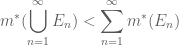 $\displaystyle m^*( \bigcup_{n=1}^\infty E_n ) < \sum_{n=1}^\infty m^*(E_n)$ if $m^*( \bigcup_{n=1}^\infty E_n )$ is finite,we must have

$\displaystyle m^*( \bigcup_{n=1}^\infty E_n ) = \sum_{n=1}^\infty m^*(E_n)$ if $m^*( \bigcup_{n=1}^\infty E_n )$ is infinite.

30 April, 2013 at 9:25 am

Luqing Ye

A remark to Lemma 8:

“Let $E\subset \mathbf{R}^d$ be an open set. Then $E$ can be expressed as the countable union of almost disjoint boxes (and, in fact, as the countable union of almost disjoint closed cubes).”

I think that the following is also true:

Let $E\subset \mathbf{R}^d$ be an open set. Then $E$ can be expressed UNIQUELY as the countable union of disjoint open boxes.

30 April, 2013 at 9:43 am

Luqing Ye

A remark to Lemma 9(outer regularity)

Outer regularity can also be stated as this way,which is also the way I prefer:

$\displaystyle m^*(\bigcup_{j\in \mathbb{N}^+}E_j)=\lim_{N\to\infty}m^*(\bigcup_{j=1}^{N}E_j)$

1 May, 2013 at 10:12 am

Luqing Ye

A remark to lemma 11(countable additivity),(2).

This lemma tells us the simple fact that disjoint Lebesgue measurable sets has the property of countable additivity,the proof,however,is rather tough,and long.

When faced with such a proof,I usually do not like to read it,because even though I read it,the proof still belongs to the one who find out it.Mathematics,do not like other subjects such as language——Even if you see a proof many times , it still do not belongs to you.In order to truely understand a proof,you have to find it out yourself,or,if the proof is so hard that it does not worth to invest too much time in it, at least you should try to simplify it or rewrite it in your own way,or decompose it in simpler steps.

So I find a proof myself,I think my proof is a bit simpler than Mr.Tao’s proof.Now let me start the proof.

As a preliminary,I have already proved that a set is L-measurable iff it satisfy the Carathéodory criterion.

Let $T=\bigcup_{j\in \mathbf{N}^+}E_j$ ,We first prove that $T$ is L-measurable,that is ,according to Caratheodory criterion, $\forall A\in\mathbf{R}^d$ , $m^*(A)=m^*(A\backslash T)+m^*(A\bigcap T)$ .

According to the sub-additivity property of outer measure,we know that $m^*(A)\leq m^*(A\backslash T)+m^*(A\bigcap T)$ ,so we only need to prove that $m^*(A)\geq m^*(A\backslash T)+m^*(A\bigcap T)$ .

According to the Morgan law,we just need to prove that

$\displaystyle m^*(A)\geq m^*(A\backslash T)+m^*(\bigcup_{j\in \mathbf{N}^+}(A\bigcap E_j))$ .

According to the outer regularity(Lemma 9,see also my comment https://terrytao.wordpress.com/2010/09/09/245a-notes-1-lebesgue-measure/#comment-227019 ),we just need to prove that

$\displaystyle m^*(A)\geq m^*(A\backslash T)+\lim_{N\to\infty}m^*((\bigcup_{i=1}^N(A\bigcap E_i)))$ .

According to the Monotonicity property of outer measure,we know that $\displaystyle m^*(A\backslash T)+\lim_{N\to\infty}m^*(\bigcup_{i=1}^N(A\bigcap E_i))\leq m^*(A\backslash \lim_{N\to\infty}(\bigcup_{j=1}^NE_j))+\lim_{N\to\infty}m^*(\bigcup_{i=1}^N(A\bigcap E_i))$ .

So we just need to prove that

$\displaystyle m^*(A)\geq m^*(A\backslash \lim_{N\to\infty}(\bigcup_{j=1}^NE_j))+\lim_{N\to\infty}m^*((\bigcup_{i=1}^N(A\bigcap E_i)))$ ………….(1)

According to the L-measurability of $E_j$ (together with the mathematical induction),we know that

$\displaystyle m^*(A)=m^*(A\backslash \lim_{N\to\infty}(\bigcup_{j=1}^NE_j))+\lim_{N\to\infty}m^*(A\bigcap(\bigcup_{i=1}^NE_i))$ ,

so (1) holds.So $T$ is L-measurable.Now we prove that

$\displaystyle m(\bigcup_{j\in \mathbf{N}^+}E_j)=\sum_{j\in \mathbf{N}^+}m(E_j)$ .

According to the outer regularity(Lemma 9,see also my comment https://terrytao.wordpress.com/2010/09/09/245a-notes-1-lebesgue-measure/#comment-227019 ),we have

$\displaystyle m(\bigcup_{j\in \mathbf{N}^+}E_j)=\lim_{N\to\infty}m^*(\bigcup_{j=1}^NE_j)$ .

Then according to the finite additivity of disjoint L-measurable sets(The finite additivity of disjoint L-measurable sets can be easily proved by using Caratheodory criterion together with the mathematical induction.),we have $\displaystyle m(\bigcup_{j\in J}E_j)=\lim_{N\to\infty}m^*(\bigcup_{j=1}^NE_j)=\lim_{N\to\infty}\sum_{j=1}^Nm^*(E_j)$ .

Done. $\Box$

2 May, 2013 at 12:09 am

Luqing Ye

———-
A remark to Exercise 11,(2),(Downward
monotone convergence) .

It seems that the condition here is stronger than in Mr.Tao’s book
“Analysis”,exercise 18.2.3.

In that book,the Downward monotone convergence theorem is stated as
follows:

Show that if $A_1\supseteq A_2\supseteq A_3\cdots$ is a decreasing
sequence of measurable sets,and $m(A_1)\prec +\infty$ ,then we have
$m(\bigcap_{j=1}^{\infty}A_j)=\lim_{j\to\infty}m(A_j)$ .

At that time,my proof to that exercise is stated as follows:
——————————–

Firstly,by the $\sigma-$ algebra property,we know that
$m(\bigcap_{j=1}^{\infty}A_j)$ is measurable.

Then,it is easy to verify that $\displaystyle A_1\backslash\bigcup_{i=1}^{\infty}(A_i\backslash A_{i+1})=\bigcap _{i=1}^{\infty}A_i$ .So $\displaystyle m(A_1\backslash\bigcup_{i=1}^{\infty}(A_i\backslash A_{i+1}))=m(\bigcap_{i=1}^{\infty}A_i)$ .

According to the finite additivity of disjoint measurable sets,we have
$\displaystyle m(A_1\backslash\bigcup_{i=1}^{\infty}(A_i\backslash A_{i+1}))=m(A_1)-m(\bigcup_{i=1}^{\infty}(A_i\backslash A_{i+1}))$ .
( $m(A_1)$ is finite,so the operation of minus makes sense).

According to Exercise 11,(1)(Upward monotone convergence),we have
$\displaystyle m(\bigcup_{i=1}^{\infty}(A_i\backslash A_{i+1}))=m(A_1)-\lim_{j\to\infty}(A_j)$ ,so $\displaystyle m(\bigcap_{j=1}^{\infty}A_j)=m(A_1\backslash\bigcup_{i=1}^{\infty}(A_i\backslash A_{i+1}))=\lim_{j\to\infty}A_j$ .

————————-

But,surprizingly,the condition in Exercise 11,(2) is a bit
stronger than in Mr.Tao’s book, $m(A_1)$ does not need to be
finite,in the case of when $m(A_1)$ is not finite, $m(A_j)(j\geq 2)$ is
finite,the theorem also holds!

So I think I need to change my proof a bit to prove this stronger
theorem.Now I figure out it,I even do not need to change my
proof,because ”the stronger theorem” only make use of the fact that
the first finite elements of a sequence do not affect its limit!HaHaHaHa…

2 May, 2013 at 9:19 pm

Luqing Ye

A remark to Exercise 13,(1).

This exercise is stated as follows:

“Show that if the $E_n$ are all Lebesgue measurable, and converge pointwise to $E$ , then $E$ is Lebesgue measurable also.”

I love this exercise,because this exercise makes me think again about the distinction between the uniform convergence and pointwise convergence.

I think uniform convergence correspond to the finite intersection of sets,and pointwise convergence correspond to the infinite(countable or uncountable) intersection of sets.

In this particular exercise,pointwise convergence correspond to the countable intersection of sets(Because $(E_n)_{n=1}^{\infty}$ is countable).

2 May, 2013 at 11:00 pm

Luqing Ye

A remark to Exercise 15,(inner regularity).

Inner regularity is just a counterpart to outer regularity.Just consider the complement of the measurable set $E$ will be enough.

But now I still have something to think.In the case of outer regularity(lemma 9),why $U$ has to be open?

Open set.I frequently see open set in real analysis.Why open set?I think one reason mathematician like open set,is that,open set has a good property:

Every open set in $\mathbf{R}^d$ can be expressed uniquely into at most countable union of open boxes.

This property makes us define the outer measure more conveniently.Because it is easy to define the volume of at most countable union of open boxes.

So if we don’t use open set in outer measure,to reach the same effect,we have to use at most countable union of elementary boxes instead,this becomes more inconvenient in language.

3 May, 2013 at 6:28 am

Luqing Ye

A remark to Exercise 21:

In my comment https://terrytao.wordpress.com/2010/09/04/245a-prologue-the-problem-of-measure/#comment-226452,I have proved this result in the case of Jordan measure.

Now I begin to prove this result in the case of Lebesgue measure.Of course,I will try to base my argument on my proof in the case of Jordan measure.

So the proof becomes simple,based on two facts:

1.A Lebesgue measurable set can be arbitrarily approximated by a Jordan measurable set.

2.A linear transformation from $\mathbf{R}^d$ to itself will not transform a set whose outer measure is very small to a set whose outer measure is far larger.

Fact 1 can be easily proved by the definition of Lebesgue measure.

Fact 2 can be easily proved by the change of variables formula in Jordan measure.

3 May, 2013 at 9:37 pm

Luqing Ye

In fact,I think if there is no irrationional number in mathematical world,i.e,there exists only rational number system in mathematics,then Jordan measure will be enough,and we don’t need Lebesgue measure.

Unfortunately(Or fortunately?),there is real number system,so we need Lebesgue measure.

Jordan measure is suitable for $\mathbf{Q}$ ,Lebesgue measure is suitable for $\mathbf{R}$ .

So if we only use Jordan measure in $\mathbf{R}$ ,that will be not enough.

Jordan measure is dense,but Lebesgue measure is complete!

Complete stuff is real infinity,and dense stuff is not real infinity.Like a natural number,a natural number is finite,but the set of all the natural number is infinite!

4 May, 2013 at 7:41 am

Luqing Ye

A remark to Exercise 27:
———–
What is the use of the condition “continuously differentiable” ?

Continuously differentiable reminds of the motion of a mass point in physics. $S(t)$ is continuously differentiable.

Maybe with this condition,we can compute the length of the curve?Does a curve which has length in higher dimensional space has outer measure zero?What does a curve which has length mean?
———–

The above is what I thought when I didn’t know how to solve this problem.Now I figure out it,the condition “continuously differentiable” enable us to approximate this curve by a polygonal line very well!Note that “continuous” is also needed,otherwise,the curve may change so rapidly in an arbitrarily small scale that we can not approximate it well by using polygonal line.

28 May, 2014 at 7:00 am

Anonymous

in the remark, $\displaystyle m_{*,(J)}(E) \leq m^*(E) \leq m^{*,(J)}(E) \ \ \ \ \ (3)$ , do we have all the combinations of these inequalities?

$E=Q\cap[0,1]$ gives $\displaystyle m_{*,(J)}(E) = m^*(E) < m^{*,(J)}(E)$ and when $E$ is a Jordan measurable set, we have the equalities. I don’t have examples for
$\displaystyle m_{*,(J)}(E) < m^*(E) < m^{*,(J)}(E)$
and
$\displaystyle m_{*,(J)}(E) < m^*(E) = m^{*,(J)}(E)$ .

[Experiment with Boolean combinations of your original example ${\bf Q} \cap [0,1]$ , e.g. taking complements in $[0,1]$ , or taking unions or other combinations with translates ${\bf Q} \cap [2,3]$ of your original example. -T.]

28 May, 2014 at 7:16 am

Anonymous

I don’t quite understand the following remark:

“one does not gain any increase in power in the Jordan inner measure by replacing finite unions of boxes with countable ones.”

– Does “increase in power” for Lebesgue outer measure (which is defined by replacing finite unions of boxes with countable ones in Jordan out measure) refer to countable subadditivity?
– The asymmetry “ultimately arises from the fact that elementary measure is subadditive rather than superadditive”. Could you elaborate this point further?

28 May, 2014 at 10:08 am

Terence Tao

If one tries to define a “Lebesgue inner measure” by naive analogy with Lebesgue outer measure, that is to say by taking the sup over all countable collections of disjoint boxes inside the set, one gets exactly the same measure as Jordan inner measure. In contrast, the Lebesgue outer measure can be significantly smaller than the Jordan outer measure, and thus come much closer to measuring the “true” size of the set. In particular, Lebesgue outer measure gives the “correct” answer for the measure of a set far more often than Jordan inner or outer measure, which is what I mean by power (and countable subadditivity is of course further confirmation of this fact).

For the final remark, I am referring to the basic fact that if E and F are elementary sets (possibly overlapping), then we have the subadditivity property $m(E \cup F) \leq m(E) + m(F)$ , but not the superadditivity property $m(E \cup F) \geq m(E) + m(F)$ . This creates an asymmetry between lower and upper bounds, which is ultimately why Lebesgue outer measure obeys a useful countable subadditivity property, whereas “Lebesgue inner measure” as naively defined above enjoys no comparable property.

29 May, 2014 at 7:38 am

Anonymous

The conclusion in Exercise 6 seems very unnatural: on one side of the equality, $E$ is approximated by finite union of boxes from inside; one the other side, it is approximated by countable union of boxes from outside. Does the asymmetry here arise from the same fact?

In the elementary and Jordan measure theory (and Riemann integration), one can see the symmetry such as inner and outer measure, lower and upper integral and the terms “measurable”, “integrable” are defined when the “symmetric” concepts are equal to each other. Can one say that in Lebesgue measure and integration theory, such symmetry does not exist any more (one does have the correct version of the Lebesgue inner measure though, things are note defined as “when lower and upper or inner and outer stuffs match with each other…”) and it is this asymmetry that makes the Lebesgue theory more “powerful” than the Riemann integration theory?

29 May, 2014 at 7:12 am

Anonymous

I don’t see why “If one tries to define a “Lebesgue inner measure” by naive analogy with Lebesgue outer measure, one gets exactly the same measure as Jordan inner measure”.

Let $\displaystyle m_*(E):=\sup_{\cup_n^\infty B_n\subset E} \sum_{n=1}^\infty |B_n|$ for any $E\subset{\bf R}^d$ be the naive definition. I’m trying to show as you said that
$\displaystyle m_*(E)=m_{*,(J)}(E)$ .

The direction $m_*(E)\geq m_{*,(J)}(E)$ is obvious since one can replace the finite union with the infinite one using empty sets. I don’t see why $m_*(E)\leq m_{*,(J)}(E)$ is true. I thought Lemma 7 might be useful since one could have the estimate
$\displaystyle m_*(E)-\epsilon\leq\sum^\infty_{n=1}|B_n|=m^*(\cup_{n=1}^\infty B_n)$
$\displaystyle \leq m^*(A)=m(A)\leq m_{*,(J)}(E)$ if one has the elementary set $A$ such that
$\displaystyle \cup_{n=1}^\infty B_n\subset A\subset E$ . But I don’t see why such $A$ exists.

Could you explain why one can achieve the second inequality?

29 May, 2014 at 7:40 am

Terence Tao

For any $X < \sum_{n=1}^\infty |B_n|$ , one can find $N$ such that $\sum_{n=1}^N |B_n| \geq X$ . For instance, if $\sum_{n=1}^\infty |B_n|$ is finite, one can find $N$ such that $\sum_{n=1}^N |B_n| \geq \sum_{n=1}^\infty |B_n| - \varepsilon$ .

1 June, 2014 at 8:00 am

Peter

I don’t see why “If one tries to define a “Lebesgue inner measure” by naive analogy with Lebesgue outer measure, one gets exactly the same measure as Jordan inner measure”. Let \displaystyle m_*(E):=\sup_{\cup_n^\infty B_n\subset E} \sum_{n=1}^\infty |B_n| for any E\subset{\bf R}^d be the naive definition. I’m trying to show as you said that […]

For any X < \sum_{n=1}^\infty |B_n|, one can find N such that \sum_{n=1}^N |B_n| \geq X. For instance, if \sum_{n=1}^\infty |B_n| is finite, one can find N such that \sum_{n=1}^N |B_n| \geq \sum_{n=1}^\infty |B_n| – \vvarepsilon.

1 June, 2014 at 8:32 am

Terence Tao

An infinite sum $\sum_{n=1}^\infty x_n$ of non-negative quantities $x_n$ is the least upper bound of its partial sums $\sum_{n=1}^N x_n$ .

Also, to define inner measure in a reasonable way in this fashion, one would have to insist that the $B_n$ are disjoint or almost disjoint (if one could re-use the same box over and over again, then any set with non-trivial interior would have infinite inner measure.)

29 September, 2015 at 9:55 pm

275A, Notes 0: Foundations of probability theory | What's new

[…] to say products of closed intervals. The construction of Lebesgue measure is a little tricky; see this previous blog post for […]

12 October, 2015 at 12:35 pm

275A, Notes 2: Product measures and independence | What's new

[…] We would like to extend to a countably additive probability measure on . The standard approach to do this is via the Carathéodory extension theorem in measure theory (or the closely related Hahn-Kolmogorov theorem); this approach is presented in these previous lecture notes, and a similar approach is taken in Durrett. Here, we will try to avoid developing the Carathéodory extension theorem, and instead take a more direct approach similar to the direct construction of Lebesgue measure, given for instance in these previous lecture notes. […]

15 November, 2015 at 9:49 am

Dr. Bob

Pls i need more explanations and examples on how to compute lebegue outer measure of a set. Thank

28 March, 2016 at 11:22 am

Anonymous

A bounded function on a compact interval $[a, b]$ is Riemann integrable if and only if it is continuous almost everywhere. Is this true for $f:{\bf R^n}\to{\bf R}$ in general?

8 March, 2017 at 6:06 pm

Anonymous

I’m trying to understand Axiom 3 and Corollary 4. Without AC, is ZF enough to give the” axiom of finite choice”? For instance suppose $f:\mathbb{R}\to B$ is onto, where $B$ is finite. Can we *prove* without AC that there is a function $g:B\to\mathbb{R}$ such that $f(g(b))=b$ for each $b\in B$ .

[Finite choice can be proven without AC by induction on the cardinality of $B$ . -T.]

22 June, 2017 at 6:14 pm

Anonymous

What would be the trade-off for Definition 1 of Lebesgue measure? As you said under definition 1, Littlewood’s first principle is almost trivial. What’s the cost? What would be the advantage of the one using Carathéodory criterion? How about the one using Riesz representation theorem?

23 June, 2017 at 1:10 pm

Anonymous

Regarding Exercise 8, is there a reason why we use open sets for the outer approximation and closed sets for the inner approximation but not the other way around (closed sets for the outer and open sets for the inner)? In the Definition 1 of Lebesgue measures, can we use closed $U$ containing $E$ instead?

26 August, 2017 at 6:38 pm

Anonymous

In the proof of Lemma 10(ii), does one have to reduce to the case when $E$ is compact? In order to apply Exercise 5, one only needs one of the sets being compact. On the other hand the finite union of the closed cubes $Q_j$ is compact.

28 August, 2017 at 1:53 pm

Terence Tao

If $E$ is non-compact then it becomes possible for $m^*(E)$ to be infinite, and so one cannot easily cancel it at the end of the proof of Lemma 10(ii).

28 August, 2017 at 4:43 pm

Anonymous

I have a dumb question that I don’t know how to answer it myself. The inner regularity and out regularity imply that given any measurable set $E\subset{\bf R}^d$ and $\varepsilon>0$ , there exists an open set $O\supset E$ and a closed set $F\subset E$ such that
$\displaystyle m(O\setminus E)\leq \varepsilon$
and
$\displaystyle m(E\setminus F)\leq \varepsilon$

Is it still true if we switch “open” and “closed” in the statement above? (Do we have approximation by open sets from inside and closed sets from outside?)

29 August, 2017 at 7:25 am

Terence Tao

Hint: try to think of a set which is “large” but contains no open sets (i.e. has empty interior). Or, conversely, think of a set which is “small” but has huge closure.

9 November, 2017 at 7:01 pm

Anonymous

How should one understand “large” and “small” in the hint? In terms of cardinality or something else?

The first/only thing that has empty interior I can come up with is the Cantor set $C$ . But it seems that it could not be a desired example: there indeed exists an open set $O$ (namely the empty set) contained in $C$ such that $m(C\backslash O)\leqslant\varepsilon$ . Also since $C$ is closed, one has $m(F\backslash C)=0\leqslant\varepsilon$ . :-(

9 November, 2017 at 9:54 pm

Terence Tao

Second hint: a set has no interior if and only if its complement is dense.

28 August, 2017 at 5:01 pm

Anonymous

Exercise 20 is done in Stein-Shakarchi by approximation of open sets. Is it possible to use the monotone class theorem, which is in later notes? Would it be a circular argument?

29 August, 2017 at 7:26 am

Terence Tao

Try it! The proof of the monotone class lemma is not exceedingly difficult, and does not require the construction of Lebesgue measure.

26 October, 2017 at 8:30 am

haonanz

Hello Prof. Tao, This might be a really trivial thing. But In the proof of lemma 8, wouldn’t it be more necessary to show that ${{\mathcal Q}^*}$ is actually non-empty? I think intuitively it would be true, as I was thinking about an open interval case in $\mathbb{R}$ , but I am not sure how to show this for an arbitrary open set in $\mathbb{R}^d$ . Thanks,

26 October, 2017 at 8:15 pm

Terence Tao

Actually, ${\mathcal Q}^*$ will be empty if and only if $E$ is empty, since (as shown in the proof) $E$ will be the union of all the cubes in ${\mathcal Q}^*$ .

17 November, 2017 at 5:18 pm

Anonymous

Given a bounded subset $E$ of ${\bf R}^d$ , it is not necessarily true that $E$ can be written as a countable union of Jordan measurable sets since there exits bounded non-Lebesgue measurable sets and any Jordan measurable sets are Lebesgue measurable.

In this argument, one would have to use the axiom of choice since one needs a non-Lebesgue measurable set.

Is it possible without using AC to show that any bounded set is not necessarily a countable union of Jordan measurable sets?

3 September, 2019 at 7:17 pm

Confused Student

One thing that is puzzling me is whether or not there an assumption that $\mathbb{R}^n$ is equipped with the Euclidean distance metric when defining the Lebesgue Measure.

It feels like this is the case, but it is never explicitly stated. For instance if we equip $\mathbb{R}^n$ with a different metric, say one based on the infinity norm, then we can still define the Lebesgue measure on that space, but now volumes have the property that they are invariant under isometries of the plane, whereas the underlying distance metric is not.

Thought?

4 September, 2019 at 8:32 am

Terence Tao

Good questions! Usually, ${\bf R}^n$ is understood to be n-dimensional Euclidean space, and in particular is indeed equipped with the Euclidean metric. If one wanted to explicitly omit this structure, one should probably talk about an “ $n$ -dimensional real vector space” or something similar instead of ${\bf R}^n$ .

On the other hand, it is true that every locally compact abelian group comes with a Haar measure, which is unique up to multiplication by scalars. In the case of Euclidean space ${\bf R}^n$ , Lebesgue measure is the unique Haar measure $m$ that obeys the normalisation $m([0,1]^n)=1$ ; see Exercise 23 of this blog post. In other words, the only role that the Euclidean metric really plays in the definition of Lebesgue measure is in defining the set used to normalise Lebesgue measure, in this case the unit cube. One could use a different set for this normalisation, for instance one could define two-dimensional Lebesgue measure to be the unique Haar measure that assigns a measure of $\pi$ to the unit disk $\{ x \in {\bf R}^2: \|x\| \leq 1 \}$ . (This may seem like an idiosyncratic way to define Lebesgue measure, but it has some advantages, for instance it makes it instantly obvious that Lebesgue measure is rotation-invariant.) More generally, one could define Lebesgue measure using the unit ball in one’s favourite norm on ${\bf R}^n$ , although the computation of the Lebesgue measure of such a ball may require some effort.

18 March, 2022 at 4:10 pm

sin

Dear Professor Tao:
For exercise 1.2.25 in the book (continuously differentiable curves), can we say that the condition $d \geq 2$ is there to ensure that when we cover the curve by d-dimensional balls (boxes), though more is required for smaller balls (or boxes), the positive effect of “adding up many quantities” is exceeded by the ability to shrink each quantity by a greater factor, so that one is still able to upper bound the total volume?

[Yes. Also for $d=1$ there are easy counterexamples – T.]

	Anonymous on On product representations of…
	Alex Gunning on A symmetric formulation of the…
	Terence Tao on On product representations of…
	domotorp on On product representations of…
	Terence Tao on 275A, Notes 3: The weak and st…
	Terence Tao on A symmetric formulation of the…
	Anonymous on On product representations of…
	Anonymous on 275A, Notes 3: The weak and st…
	Anonymous on 275A, Notes 3: The weak and st…
	Alex Gunning on A symmetric formulation of the…
	Anonymous on Erratum for “An inverse…
	Anonymous on Erratum for “An inverse…
	Anonymous on Erratum for “An inverse…
	Anonymous on 275A, Notes 3: The weak and st…
	Anonymous on It ought to be common knowledg…

245A, Notes 1: Lebesgue measure

Recent Comments

Articles by others

Diversions

Mathematics

Selected articles

Software

The sciences

Top Posts

Archives

Categories

The Polymath Blog

133 comments

Leave a comment Cancel reply

For commenters

245A, Notes 1: Lebesgue measure

Share this:

Recent Comments

Articles by others

Diversions

Mathematics

Selected articles

Software

The sciences

Top Posts

Archives

Categories

The Polymath Blog

133 comments

Leave a comment Cancel reply

For commenters