
In the previous set of notes we saw how a representation-theoretic property of groups, namely Kazhdan’s property (T), could be used to demonstrate expansion in Cayley graphs. In this set of notes we discuss a different representation-theoretic property of groups, namely quasirandomness, which is also useful for demonstrating expansion in Cayley graphs, though in a somewhat different way to property (T). For instance, whereas property (T), being qualitative in nature, is only interesting for infinite groups such as 

The definition of quasirandomness is easy enough to state:
Definition 1 (Quasirandom groups) Let
be a finite group, and let
. We say that
-quasirandom if all non-trivial unitary representations
of
is the identity for all
.)
Exercise 1 Let
has no
and
Remark 1 The terminology “quasirandom group” was introduced explicitly (though with slightly different notational conventions) by Gowers in 2008 in his detailed study of the concept; the name arises because dense Cayley graphs in quasirandom groups are quasirandom graphs in the sense of Chung, Graham, and Wilson, as we shall see below. This property had already been used implicitly to construct expander graphs by Sarnak and Xue in 1991, and more recently by Gamburd in 2002 and by Bourgain and Gamburd in 2008. One can of course define quasirandomness for more general locally compact groups than the finite ones, but we will only need this concept in the finite case. (A paper of Kunze and Stein from 1960, for instance, exploits the quasirandomness properties of the locally compact group
to obtain mixing estimates in that group.)
Quasirandomness behaves fairly well with respect to quotients and short exact sequences:
Exercise 2 Let
be a short exact sequence of finite groups
.
- (i) If
is
- (ii) Conversely, if
Informally, we will call 

The way we have set things up, the trivial group 
Exercise 3 Let
- (i) Show that if
. (Hint: use the mean zero component
of the regular representation
.) In particular, non-trivial finite groups cannot be infinitely quasirandom.
- (ii) Show that any proper subgroup
. (Hint: use the mean zero component of the quasiregular representation.)
The following exercise shows that quasirandom groups have to be quite non-abelian, and in particular perfect:
Exercise 4 (Quasirandomness, abelianness, and perfection) Let
- (i) If
-quasirandom. (Hint: use Fourier analysis or the classification of finite abelian groups.)
- (ii) Show that
is equal to
Later on we shall see that there is a converse to the above two exercises; any non-trivial perfect finite group with no large subgroups will be quasirandom.
Exercise 5 Let
of
-quasirandom, where
is the index of
Now we give an example of a more quasirandom group.
Lemma 2 (Frobenius lemma) If
is a field of some prime order
, then
is
-quasirandom.
This should be compared with the cardinality 
Proof: We may of course take 


and suppose first that 


Exercise 6 Show that for any prime
for
ranging over

Exercise 7 Let
of
Exercise 8 Show that
is
and any prime
, which follows from the results of Landazuri and Seitz.)
As a corollary of the above results and Exercise 2, we see that the projective special linear group 
Remark 2 One can ask whether the bound
, we see that it also acts projectively on the projective line
, which has
elements. Thus
, and also on the
; this latter representation (known as the Steinberg representation) is irreducible. This shows that the
,
of functions
that obey the twisted dilation invariance
for all
and
; these are known as the principal series representations. When
is the trivial character, this is the quasiregular representation discussed earlier. For most other characters, this is an irreducible representation, but it turns out that when
while being non-trivial), the principal series representation splits into the direct sum of two
-dimensional representations, which comes very close to matching the bound in Lemma 2. There is a parallel series of representations to the principal series (known as the discrete series) which is more complicated to describe (roughly speaking, one has to embed
and then use a rotated version of the above construction, to change a split torus into a non-split torus), but can generate irreducible representations of dimension
Exercise 9 Let
, the alternating group
is
-quasirandom. (Hint: show that all cycles of order
); in particular, a cycle is conjugate to its
power for all
. Also, as
,
Remark 3 By using more precise information on the representations of the alternating group (using the theory of Specht modules and Young tableaux), one can show the slightly sharper statement that
-quasirandom for
(but is only
-quasirandom for
due to icosahedral symmetry, and
-quasirandom for
due to lack of perfectness). Using Exercise 3 with the index
subgroup
, we see that the bound
If one replaces the alternating group
, is not perfect); indeed,
Remark 4 Thanks to the monumental achievement of the classification of finite simple groups, we know that apart from a finite number (26, to be precise) of sporadic exceptions, all finite simple groups (up to isomorphism) are either a cyclic group
, an alternating group
in characteristic
, it is known from the work of Landazuri and Seitz that such groups are
-quasirandom for some
-quasirandom for some
is sufficiently large depending on
, then
. It would be of interest to see if there was an alternate way to establish this fact that did not rely on the classification, as it may lead to an alternate approach to proving the classification (or perhaps a weakened version thereof).
A key reason why quasirandomness is desirable for the purposes of demonstrating expansion is that quasirandom groups happen to be rapidly mixing at large scales, as we shall see below the fold. As such, quasirandomness is an important tool for demonstrating expansion in Cayley graphs, though because expansion is a phenomenon that must hold at all scales, one needs to supplement quasirandomness with some additional input that creates mixing at small or medium scales also before one can deduce expansion. As an example of this technique of combining quasirandomness with mixing at small and medium scales, we present a proof (due to Sarnak-Xue, and simplified by Gamburd) of a weak version of the famous “3/16 theorem” of Selberg on the least non-trivial eigenvalue of the Laplacian on a modular curve, which among other things can be used to construct a family of expander Cayley graphs in 


— 1. Mixing in quasirandom groups —
Let 


This operation is bilinear and associative, but is not commutative unless

and hence

This inequality is sharp in the sense that if we set 

It turns out, though, that if one restricts one of
Proposition 3 (Mixing inequality) Let
has mean zero, then

Proof: By subtracting a constant from
Observe that 


Fix 
of 


Now, a short computation shows that 


Thus, if 


Now observe that if 

for any 


Remark 5 One can also establish the above inequality using the nonabelian Fourier transform (which is based on the Peter-Weyl theorem combined with Schur’s lemma, and is developed in this blog post); we leave this as an exercise for the interested reader.
Exercise 10 Let
be subsets of a finite
and
Conclude in particular that
and that
whenever
. (The bounds here are not quite sharp, but are simpler than the optimal bounds, and suffice for most applications.)


Thus, for instance, if 


Exercise 11 Let
for some absolute constant
, such that
. (Hint: by hypothesis, one has a non-trivial unitary representation
contains an element at distance
from the identity in operator norm, and take
One can improve this result by using a quantitative form of Jordan’s theorem; see the next section.
Exercise 12 (Mixing inequality for actions) Let
. Given functions
and
, one can define the convolution
in much the same way as before:
Show that
whenever

One can use quasirandomness to show that Cayley graphs of very large degree 
Exercise 13 Let
be a
- (i) If
are subsets of
(compare with the expander mixing lemma, Exercise 9 from Notes 1).
- (ii) Show that
-expander whenever

Unfortunately, the above result is only non-trivial in the regime 

Proposition 4 (Using quasirandomness to demonstrate expansion) Let
- (i) (Quasirandomness)
-quasirandom for some
.
- (ii) (Flattening of random walk) One has
for some
with
and
, where
and
is the
.
Then
depending only on
, if
in the flattening hypothesis, then

Proof: We allow implied constants to depend on 
(say) for some 

for any 


Exercise 14 Obtain an alternate proof of the above result that proceeds directly from the spectral decomposition of the adjacency operator
into eigenvalues and eigenvectors and quasirandomness, rather than through Exercise 5 from Notes 2 and Proposition 3. (This alternate approach is closer in spirit to the arguments of Sarnak-Xue and Bourgain-Gamburd, though the two approaches are largely equivalent in the final analysis.)
Informally, the flattening hypothesis in Proposition 4 asserts that by time 

The following exercise extends some of the above theory from quasirandom groups to “virtually quasirandom” groups, which have a bounded index subgroup that is quasirandom, but need not themselves be quasirandom.
Exercise 15 (Virtually quasirandom groups) Let
- (i) If
- (ii) If
for some
, and
.
— 2. An algebraic description of quasirandomness (optional) —
As defined above, quasirandomness is a property of representations. However, one can reformulate this property (at a qualitative level, at least) in a more algebraic fashion, by means of Jordan’s theorem:
Theorem 5 (Jordan’s theorem) Let
for some
. Then
, where
A proof of this theorem (giving a rather poor value of 


Jordan’s theorem can be used to give a qualitative description of quasirandomness, providing a converse to Exercises 3 and 4:
Exercise 16 Let
be an integer. Let
, where
Conclude in particular that any finite simple nonabelian group of cardinality greater than
By using the classification of finite simple groups more carefully, Nikolov and Pyber were able to replace 


— 3. A weak form of Selberg’s 3/16 theorem (optional) —
Remark 6 This section presumes some familiarity with Riemannian geometry, as well as the functional analysis of Sobolev spaces and distributions. See for instance this blog post for a very brief introduction to Riemannian geometry, and these two previous posts for an introduction to distributions and Sobolev spaces.
We now give an application of quasirandomness to establish the following result, first observed explicitly by Lubotsky, Phillips and Sarnak as a corollary of a famous theorem of Selberg:
Theorem 6 (Selberg’s expander construction) If
is a symmetric set of generators of
that does not contain the identity, then the Cayley graphs
form a one-sided expander family, where
is the obvious projection homomorphism, and
This is the 
In the property (T) approach to expansion, one passed from discrete groups such as 
We now therefore digress from the topic of expansion to recall the geometry of the hyperbolic plane. It will be convenient to switch between a number of different coordinatisations of this plane. Our primary model will be the half-plane model:
Definition 7 (Poincaré half-plane model) The Poincaré half-plane is the upper half-plane
with the Riemannian metric
. The (left) action of
One easily verifies that this gives an isometric action on
.
Exercise 17 Verify that
; thus
.
Note that in some of the literature, a right action is used instead of a left action, leading to some reversals in the notational conventions used below, but this does not lead to any essential changes in the arguments or results.
Exercise 18 Show that the distance
between two points
is given by the formula

We can also use the model of the Poincaré disk 

Exercise 19 Show that the Cayley transform
is an isometric isomorphism from the half-plane
.
Expressing an element 


![{[0,\pi]}](https://s0.wp.com/latex.php?latex=%7B%5B0%2C%5Cpi%5D%7D&bg=ffffff&fg=000000&s=0&c=20201002)


The action of
A Riemannian metric on a manifold always generates a measure 


A Riemannian metric also generates a Laplace-Beltrami operator 

in the Poincaré disk model, it is

and in the half-cylinder model, it is
Again, in all cases, the Laplacian will commute with the action of
The discrete group 

and then identifying 


for any constant 


Thus
Remark 7 One can interpret the modular curve geometrically as follows. As in the previous set of notes, one can think of
(or equivalently, in
) with two marked generators
with
. We can then map
to the point
; note that the fibers of this map correspond to rotations of the lattice and marked generators, thus identifying
then corresponds to the selection of generators given by setting
to be the non-zero lattice element of smallest norm, and
to be the generator whose
and
.
The quotient 

The Laplace-Beltrami operator 


where 


in the disk model, it is

and in the half-cylinder model, it is

In particular, we have the positive definiteness property

for all

Thus 

Since 


Then 

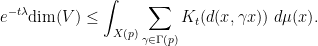
We have the following bounds:
 .
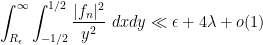
.Proof: We first establish the upper bound 


is arbitrarily close to 
We will restrict attention to smooth compactly supported functions 


where we use subscripts to denote partial differentiation, while the mean zero condition becomes
To build such functions, we select a large parameter 


and

(where the implied constant can depend on 

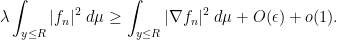
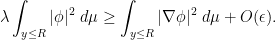
Now we show the lower bound 


where 


To deal with the non-compact portion of

and hence by Cauchy-Schwarz
Applying this to a truncated version 

![{\chi: {\bf R}^+ \rightarrow [0,1]}](https://s0.wp.com/latex.php?latex=%7B%5Cchi%3A+%7B%5Cbf+R%7D%5E%2B+%5Crightarrow+%5B0%2C1%5D%7D&bg=ffffff&fg=000000&s=0&c=20201002)


For any 


and thus we see that

for some 


Remark 8 One can in fact establish after some calculation using the theory of modular forms that
.
Now we move back towards the task of establishing expansion for the Cayley graphs 


Remark 9 One may think of
, where
, and
is the projection onto
, with each vertex of the Cayley graph being replaced by a copy of the fundamental domain
By a routine modification of Proposition 8, one can show that

(Note also that as 
Conjecture 9 (Selberg’s conjecture) One has
for all
This conjecture remains open (though it has been verified numerically for small values of 
Theorem 10 (Selberg’s 3/16 theorem) One has
for all
Selberg’s argument uses a serious amount of number-theoretic machinery (in particular, bounds for Kloosterman sums) and will not be reproduced here. The 

In the papers of by Sarnak and Xue and by Gamburd, an argument based primarily on quasirandomness that used only very elementary number theory was introduced, to obtain the following result:
Theorem 11 (Weak Selberg theorem) One has
for all primes
.
In particular, one has a uniform lower bound 


We will not quite prove Theorem 11 here, but instead establish the following even weaker version which uses the same ideas, but in a slightly less computation-intensive fashion (at the cost of some efficiency in the argument):
Theorem 12 (Even weaker Selberg theorem) One has
for all primes
Of course, this result is still strong enough to supply a uniform lower bound on
Before we prove Theorem 12 (a spectral gap in the continuous world), let us show how it can be transferred to deduce Theorem 6 (a spectral gap in the discrete world). Suppose for contradiction that Theorem 6 failed. Then we can find a finite symmetric generating set 


 independent of
 The idea now is to pass from this nearly-invariant discrete set 
We turn to the details. Let 


![{f_n: X(p_n) \rightarrow [0,1]}](https://s0.wp.com/latex.php?latex=%7Bf_n%3A+X%28p_n%29+%5Crightarrow+%5B0%2C1%5D%7D&bg=ffffff&fg=000000&s=0&c=20201002)
This function equals 


The curve 


where the bound is uniform in 


if
be the mean-free component of

for
On the other hand, 


Since 

for 

We now turn to the proof of Theorem 12. The first step is to show that the only source of spectrum below
Proposition 13 (Discrete spectrum below
. Then there exists a non-zero
such that
(in the distributional sense).
Note that while 

Proof: For notational simplicity, we will just prove the claim in the 


As before, we can take the
Using Hardy’s inequality as in the proof of Proposition 8, we see that

for any
and thus we see that
for some 

for all sufficiently large 


and thus
Taking limits in weak 


Sending 

for any

Perturbing 
for all such 
Exercise 20 Establish the above proposition for general
Exercise 21 Show that for any
on
We will also need a variant of the above proposition:
Lemma 14 (Eigenfunctions do not concentrate in cusps) Let
. Then there is a compact subset
of
on
, one has
where the implied constant is independent of
is the covering map.

The lemma is basically proved by applying Hardy’s inequality to each cusp of
Now we can start using quasirandomness. Let 

By the above proposition, this is a non-trivial Hilbert space. From Exercise 21, 
Lemma 15 (Quasirandomness) If
To complement this quasirandomness to get expansion, we need a flattening property, as in Proposition 4. In the discrete world, we applied a flattening property to the distribution 

We first recall the formula for the heat kernel on the hyperbolic plane
Exercise 22 Show that the heat operator
where
is the kernel
(Hint: There are two main computations. One is to show that
obeys the heat equation, which in half-cylindrical coordinates means that one has to verify that
The other is to show that
for small


For our purposes, we only need a crude upper bound on the heat kernel:
Exercise 23 With the notation of the preceding section, show that
when
and
.

In our applications, the polynomial factors 

The right-hand side evaluates to 

Remark 10 From Exercise 23, we see that the probability measure
concentrates around the region
; thus on the hyperbolic plane, Brownian motion moves “ballistically” away from its starting point at a unit speed, in contrast to the situation in Euclidean geometry, where after time
. One can see this phenomenon also from the heat equation (7), which when expressed in terms of the probability density
becomes a Fokker-Planck equation
with unit diffusion and drift speed
. Since
to concentrate in the region
, as is indeed the case.

We let

for 


where 

for all
This will be our starting point to get a lower bound on 
However, this turns out to be a little unfavourable because the integrand on the right-hand side does not behave well enough at cusps. However, if one uses Lemma 14 first (assuming that 

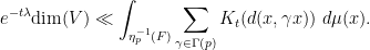
Because the sum here is

We now insert the bound in Exercise 23, as well as the bound 

Because 
Exercise 24
- (i) For any
, show that
, where
is the Frobenius norm of the matrix
.
- (ii) More generally, if
for some constant
depending only on
Inserting these bounds, we obtain

Decomposing according to the integer part 

where 

So one is left with the purely number-theoretic task of estimating 


The key is then the following “flattening lemma”, that shows that 
Lemma 16 (Flattening lemma) For any
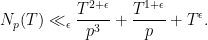
Proof: Using the definition of 

subject to the congruences

and the bounds
Since 


Now we proceed as follows. The number of integers 


giving the claim.
Remark 11 One can obtain improved bounds to
) by using more advanced tools, such as bounds on Kloosterman sums. Unfortunately, such improvements do not actually improve the final constants in this argument. (Kloosterman sums do however play a key role in the proof of Theorem 10, which proceeds by a different, and more highly arithmetic, argument.)
A routine calculation then finishes off the proof of Theorem 12:
Exercise 25 Using the above lemma, show that the right-hand side of (9) is
for any
and

Remark 12 An inspection of the above argument shows that the
term in (10) is the main obstacle to improving the
constant. This term ultimately can be “blamed” for the relatively large value of the heat kernel
bound given here to
; see the paper of Gamburd for details. Unfortunately, the fraction

30 comments
Comments feed for this article
18 December, 2011 at 5:39 pm
254B, Notes 1: Basic theory of expander graphs « Another Word For It
[…] 254B, Notes 3: Quasirandom groups, expansion, and Selberg’s 3/16 theorem […]
20 December, 2011 at 6:31 am
Wolfgang Moens
Exercise 15: I think the proof of the “in particular”-part of the exercise needs the extra assumption of “non-abelianness”. Am I missing something?
[Corrected, thanks – T.]
21 December, 2011 at 12:52 pm
Lior Silberman
The best known bound toward Selberg’s Conjecture is , due to Kim-Sarnak.
The conjecture has been verified numerically for and
and  by Booker-Strömbergsson (the resulting expanders would be the Schreyer graphs on
  rather than Cayley graphs but this isn’t much of an issue).
At the moment the conjecture cannot be verified numerically in general. The problem is that when is an exact eigenvalue, no numerical computation can show that the eigenvalue is not fractionally smaller. The Langlands Conjectures predict when this occurs; in many cases (when the Langlands-Tunnell Theorem applies) Booker-Strömbergsson) then rigorously show that there is an eigenfunction at exactly
  . Since the numerical method does count the eigenvalues, Selberg’s Conjecture follows. However, this does not work all the time.
The first case where this difficully arises (an “icosahedral representation”) occurs for .
.
[References added, thanks! – T.]
26 December, 2011 at 9:54 pm
A variant of Kemperman’s theorem « What’s new
[…] are arcs of a circle. For quasirandom , one can do much better than these bounds, as discussed in this recent blog post; thus, the abelian case is morally the worst case here, although it seems difficult to convert this […]
8 January, 2012 at 10:43 am
vipulnaik
Your statement of Jordan’s theorem misses the additional fact that the abelian subgroup is normal in the group (i.e., what you’ve written is correct but not the full theorem). Also, to obtain the second para of Exercise 15, the first para should read “proper normal subgroup” instead of “proper subgroups”. We do need to use the stronger assumption of “normal” in order to obtain the result you state in the second para of Exercise 15 involving finite simple non-abelian groups.
[Corrected, thanks – T.]
9 January, 2012 at 3:10 am
Wolfgang Moens
I have another, rather naive, question. In this post, Jordan’s theorem yields an abelian subgroup that is also normal. But, in one of the previous posts (“The Jordan-Schur theorem”), there was no mention of the existence of an abelian subgoup that was, in addition, normal. Is this just a coincidence, or is there something behind this?
E.g.: would it really be harder to generalize Jordan to Jordan-Schur if one wants to include the normality of the subgroup?
9 January, 2012 at 9:48 am
Terence Tao
Well, as long as one doesn’t care about the constants, this is straightforward, because any subgroup H of a group G of some index K will always contain a normal subgroup of G of index at most K! (namely, the kernel of the left action of G on the coset space G/H, or equivalently the intersection of all the conjugates of H).
10 January, 2012 at 2:29 am
Anonymous
Oh, yes. Thanks! =)
9 January, 2012 at 3:57 am
Wolfgang Moens
P.S.: Sorry, I have just noticed that I had not read vipulnaik’s message before posting my own.
13 January, 2012 at 7:49 pm
254B, Notes 4: The Bourgain-Gamburd expansion machine « What’s new
[…] of an infinite Cayley graph on a group with Kazhdan’s property (T). The second, discussed in Notes 3, is to combine a quasirandomness property of the group with a flattening hypothesis for the random […]
5 February, 2012 at 10:23 am
MK
Shouldn’t exercise 4, ii) state “G is 2-quasirandom iff it is perfect” instead of “not perfect”? [Corrected, thanks – T.]
5 February, 2012 at 11:32 am
254B, Notes 5: Product theorems, pivot arguments, and the Larsen-Pink non-concentration inequality « What’s new
[…] non-concentration, product theorems, and quasirandomness. Quasirandomness was discussed in Notes 3. In the current set of notes, we discuss product theorems. Roughly speaking, these theorems assert […]
13 February, 2012 at 4:51 pm
254B, Notes 6: Non-concentration in subgroups « What’s new
[…] the last three notes, we discussed the Bourgain-Gamburd expansion machine and two of its three ingredients, […]
1 March, 2012 at 5:26 pm
254B, Notes 7: Sieving and expanders « What’s new
[…] a consequence of Proposition 4 of Notes 3, the following claim was shown: Proposition 7 Let be a -quasirandom finite group, is a […]
28 November, 2012 at 5:32 pm
Multiple recurrence in quasirandom groups « What’s new
[…] Geom. Func. Anal.. This paper builds upon a paper of Gowers in which he introduced the concept of a quasirandom group, and established some mixing (or recurrence) properties of such groups. A -quasirandom group is a […]
11 December, 2012 at 9:04 pm
Mixing for progressions in non-abelian groups « What’s new
[…] starting motivation for this paper was a question posed in this foundational paper of Tim Gowers on quasirandom groups. In that paper, Gowers showed (among other things) that if was a quasirandom group, patterns such […]
12 December, 2012 at 5:37 am
Fred Lunnon
Remark 3 : for “isocahedral symmetry” read “icosahedral symmetry” . WFL
[Corrected, thanks – T.]
17 December, 2012 at 8:23 am
Uwe Stroinski
In the proof of Proposition 3 (mixing inequality) you write eigenvalue and mean eigenvalue
  .
.
[Corrected, thanks – T.]
7 February, 2013 at 12:09 am
Uwe Stroinski
Can you or a reader please help me with exercise 10. I can show the first inequality and I understand that one can use this to quantify that the number of places at which the convolution is small cannot be large. How does that help to prove the first inequality after ‘conclude in particular that’?
7 February, 2013 at 8:12 am
Terence Tao
You might find it easier to first establish the second conclusion (i.e. that whenever
  ) before establishing the first (which is equivalent to the second).
2 May, 2013 at 4:28 pm
Quasirandom groups and a cheap version of the Brauer-Fowler theorem | What's new
[…] for groups, the modern study of which was initiated by Gowers, and is discussed for instance in this previous post. It gives the following slightly weaker version of Corollary […]
7 November, 2014 at 2:07 pm
Doron Puder
Dear T.,
1) In Proposition 4, shouldn’t the ‘flattening of random walk’ condition be defined by the restriction of \mu to sum-zero functions? (Otherwise, ||\mu^{*n}||=1 for all n).
2) I suspect the 1/n term in Exercise 13 (ii) is unnecessary. I think one can prove the claim for \epsilon \le 1-\sqrt(n/(Dk)) using Proposition 3 on the eigenfunction of the largest non-trivial eigenvalue (in absolute value) and the characteristic function of S.
[(2) corrected, thanks – T.]
7 November, 2014 at 2:16 pm
Doron Puder
Please ignore the first remark. (it’s the l2-norm of a vector, not operator norm of the operator).
15 August, 2015 at 10:51 pm
A wave equation approach to automorphic forms in analytic number theory | What's new
[…] Using the Weil bound on Kloosterman sums to derive Selberg’s 3/16 theorem on the least non-trivial eigenvalue for on (discussed previously here); […]
12 November, 2015 at 12:52 pm
gninrepoli
Applying the improved estimate for the in Theorem 7 (“J.-M. Deshouillers and H. Iwaniec, Kloosterman sums and Fourier coefficients of cusp forms, Invent. Math. 70 (1982), 219-288”; p.233), you can reduce the degree of an integer
  .Will this affect the estimates of Theorem 11, and with the prospect of Theorem 12 (p.236,237)? Thank you.
13 November, 2015 at 2:54 am
gninrepoli
By Theorem 10.11 implies the assertion in Theorem 12![K^{2}(C,D,N,R,S) = CS(RS+N)(C+DR)+C^{2} DS\sqrt[]{(RS+N)R}+D^{2}NRS^{-1}](https://s0.wp.com/latex.php?latex=K%5E%7B2%7D%28C%2CD%2CN%2CR%2CS%29+%3D+CS%28RS%2BN%29%28C%2BDR%29%2BC%5E%7B2%7D+DS%5Csqrt%5B%5D%7B%28RS%2BN%29R%7D%2BD%5E%7B2%7DNRS%5E%7B-1%7D&bg=ffffff&fg=545454&s=0&c=20201002) , but I somehow doubt take that on Selberg hypothesis should be the same expression.Let Selberg conjecture is true, then
, but I somehow doubt take that on Selberg hypothesis should be the same expression.Let Selberg conjecture is true, then  in Theorem 9. It turns out that in Theorem 12 expression
 ![C^{2} DS\sqrt[]{(RS+N)R}](https://s0.wp.com/latex.php?latex=C%5E%7B2%7D+DS%5Csqrt%5B%5D%7B%28RS%2BN%29R%7D&bg=ffffff&fg=545454&s=0&c=20201002) has no place in this form. Or is it all true? I do not know if you could give your comment, if you do not complicate. Thank you.
has no place in this form. Or is it all true? I do not know if you could give your comment, if you do not complicate. Thank you.
17 April, 2020 at 3:46 am
ConstantinK
Using remark 5, do you agree that on can improve Proposition 3 to the following: for all
  . So we also get some sharper bounds in later exercises.
17 April, 2020 at 10:15 am
Terence Tao
I don’t see how to get such a good dependence on D. If one could get such a gain then one could immediately improve the exponents in a number of existing results in the literature, e.g., https://www.cambridge.org/core/journals/mathematical-proceedings-of-the-cambridge-philosophical-society/article/mixing-for-threeterm-progressions-in-finite-simple-groups/3871BEAF10295F669BAFCA2C70BF0745
18 April, 2020 at 5:22 am
ConstantinK
Ahh now I see my mistake – thank you. I just used blindly the equation from Fourier Analysis for general compact groups:
where all the integration takes place with respect to the Haar probability measure and I forgot that the 2-norm in this problem is not with respect to the Haar probability measure of .
.
25 February, 2022 at 10:13 pm
pr.likelihood - Show that $mathrm{SL}_2(mathbb{F}_p)$ is quasi-random Answer - Lord Web
[…] Terry Tao offers this indirect definition of quasi-random group in his notes 3 […]