The fundamental notions of calculus, namely differentiation and integration, are often viewed as being the quintessential concepts in mathematical analysis, as their standard definitions involve the concept of a limit. However, it is possible to capture most of the essence of these notions by purely algebraic means (almost completely avoiding the use of limits, Riemann sums, and similar devices), which turns out to be useful when trying to generalise these concepts to more abstract situations in which it becomes convenient to permit the underlying number systems involved to be something other than the real or complex numbers, even if this makes many standard analysis constructions unavailable. For instance, the algebraic notion of a derivation often serves as a substitute for the analytic notion of a derivative in such cases, by abstracting out the key algebraic properties of differentiation, namely linearity and the Leibniz rule (also known as the product rule).
Abstract algebraic analogues of integration are less well known, but can still be developed. To motivate such an abstraction, consider the integration functional  from the space
  of complex-valued Schwarz functions
  to the complex numbers, defined by
where the integration on the right is the usual Lebesgue integral (or improper Riemann integral) from analysis. This functional obeys two obvious algebraic properties. Firstly, it is linear over  , thus
and

for all  and
and  . Secondly, it is translation invariant, thus
for all  , where
  is the translation of
  by
by  . Motivated by the uniqueness theory of Haar measure, one might expect that these two axioms already uniquely determine
  after one sets a normalisation, for instance by requiring that

This is not quite true as stated (one can modify the proof of the Hahn-Banach theorem, after first applying a Fourier transform, to create pathological translation-invariant linear functionals on that are not multiples of the standard Fourier transform), but if one adds a mild analytical axiom, such as continuity of (using the usual Schwartz topology on ), then the above axioms are enough to uniquely pin down the notion of integration. Indeed, if is a continuous linear functional that is translation invariant, then from the linearity and translation invariance axioms one has

for all  and non-zero reals . If is Schwartz, then as
  , one can verify that the Newton quotients
  converge in the Schwartz topology to the derivative
  of , so by the continuity axiom one has

Next, note that any Schwartz function of integral zero has an antiderivative which is also Schwartz, and so annihilates all zero-integral Schwartz functions, and thus must be a scalar multiple of the usual integration functional. Using the normalisation (4), we see that must therefore be the usual integration functional, giving the claimed uniqueness.
Motivated by the above discussion, we can define the notion of an abstract integration functional  taking values in some vector space
  , and applied to inputs in some other vector space
  that enjoys a linear action
  (the “translation action”) of some group
  , as being a functional which is both linear and translation invariant, thus one has the axioms (1), (2), (3) for all
  , scalars
  , and
, and  . The previous discussion then considered the special case when
  ,
,  ,
,  , and
, and  was the usual translation action.
Once we have performed this abstraction, we can now present analogues of classical integration which bear very little analytic resemblance to the classical concept, but which still have much of the algebraic structure of integration. Consider for instance the situation in which we keep the complex range , the translation group , and the usual translation action , but we replace the space of Schwartz functions by the space  of polynomials
  of degree at most
  with complex coefficients, where is a fixed natural number; note that this space is translation invariant, so it makes sense to talk about an abstract integration functional
  . Of course, one cannot apply traditional integration concepts to non-zero polynomials, as they are not absolutely integrable. But one can repeat the previous arguments to show that any abstract integration functional must annihilate derivatives of polynomials of degree at most :

Clearly, every polynomial of degree at most  is thus annihilated by , which makes a scalar multiple of the functional that extracts the top coefficient
  of a polynomial, thus if one sets a normalisation
for some constant , then one has

for any polynomial . So we see that up to a normalising constant, the operation of extracting the top order coefficient of a polynomial of fixed degree serves as the analogue of integration. In particular, despite the fact that integration is supposed to be the “opposite” of differentiation (as indicated for instance by (5)), we see in this case that integration is basically (-fold) differentiation; indeed, compare (6) with the identity
In particular, we see, in contrast to the usual Lebesgue integral, the integration functional (6) can be localised to an arbitrary location: one only needs to know the germ of the polynomial at a single point  in order to determine the value of the functional (6). This localisation property may initially seem at odds with the translation invariance, but the two can be reconciled thanks to the extremely rigid nature of the class , in contrast to the Schwartz class which admits bump functions and so can generate local phenomena that can only be detected in small regions of the underlying spatial domain, and which therefore forces any translation-invariant integration functional on such function classes to measure the function at every single point in space.
The reversal of the relationship between integration and differentiation is also reflected in the fact that the abstract integration operation on polynomials interacts with the scaling operation  in essentially the opposite way from the classical integration operation. Indeed, for classical integration on
  , one has

for Schwartz functions  , and so in this case the integration functional
  obeys the scaling law
In contrast, the abstract integration operation defined in (6) obeys the opposite scaling law
Remark 1 One way to interpret what is going on is to view the integration operation (6) as a renormalised version of integration. A polynomial  is, in general, not absolutely integrable, and the partial integrals
diverge as  . But if one renormalises these integrals by the factor
  , then one recovers convergence,

thus giving an interpretation of (6) as a renormalised classical integral, with the renormalisation being responsible for the unusual scaling relationship in (7). However, this interpretation is a little artificial, and it seems that it is best to view functionals such as (6) from an abstract algebraic perspective, rather than to try to force an analytic interpretation on them.
Now we return to the classical Lebesgue integral
As noted earlier, this integration functional has a translation invariance associated to translations along the real line  , as well as a dilation invariance by real dilation parameters
  . However, if we refine the class of functions somewhat, we can obtain a stronger family of invariances, in which we allow complex translations and dilations. More precisely, let
  denote the space of all functions
  which are entire (or equivalently, are given by a Taylor series with an infinite radius of convergence around the origin) and also admit rapid decay in a sectorial neighbourhood of the real line, or more precisely there exists an
  such that for every
  there exists
  such that one has the bound
whenever  . For want of a better name, we shall call elements of this space Schwartz entire functions. This is clearly a complex vector space. A typical example of a Schwartz entire function are the complex gaussians

where  are complex numbers with
  . From the Cauchy integral formula (and its derivatives) we see that if lies in , then the restriction of to the real line lies in ; conversely, from analytic continuation we see that every function in has at most one extension in . Thus one can identify with a subspace of , and in particular the integration functional (8) is inherited by , and by abuse of notation we denote the resulting functional
  as also. Note, in analogy with the situation with polynomials, that this abstract integration functional is somewhat localised; one only needs to evaluate the function on the real line, rather than the entire complex plane, in order to compute
  . This is consistent with the rigid nature of Schwartz entire functions, as one can uniquely recover the entire function from its values on the real line by analytic continuation.
Of course, the functional remains translation invariant with respect to real translation:

However, thanks to contour shifting, we now also have translation invariance with respect to complex translation:

where of course we continue to define the translation operator  for complex by the usual formula . In a similar vein, we also have the scaling law
for any  , if
, if  is a complex number sufficiently close to
  (where “sufficiently close” depends on , and more precisely depends on the sectoral aperture parameter
  associated to ); again, one can verify that
  lies in for sufficiently close to . These invariances (which relocalise the integration functional onto other contours than the real line ) are very useful for computing integrals, and in particular for computing gaussian integrals. For instance, the complex translation invariance tells us (after shifting by
  ) that

when  with , and then an application of the complex scaling law (and a continuity argument, observing that there is a compact path connecting
  to in the right half plane) gives

using the branch of  on the right half-plane for which
  . Using the normalisation (4) we thus have

giving the usual gaussian integral formula
This is a basic illustration of the power that a large symmetry group (in this case, the complex homothety group) can bring to bear on the task of computing integrals.
One can extend this sort of analysis to higher dimensions. For any natural number  , let
, let  denote the space of all functions
  which is jointly entire in the sense that
  can be expressed as a Taylor series in
  which is absolutely convergent for all choices of , and such that there exists an
  such that for any
  there is
  for which one has the bound
whenever  for all
  , where
  and
and  . Again, we call such functions Schwartz entire functions; a typical example is the function
where  is an
is an  complex symmetric matrix with positive definite real part,
  is a vector in
  , and is a complex number. We can then define an abstract integration functional
  by integration on the real slice
  :
:
where  is the usual Lebesgue measure on . By contour shifting in each of the
  variables separately, we see that is invariant with respect to complex translations of each of the
  variables, and is thus invariant under translating the joint variable
  by . One can also verify the scaling law
for complex matrices sufficiently close to the origin, where  . This can be seen for shear transformations by Fubini’s theorem and the aforementioned translation invariance, while for diagonal transformations near the origin this can be seen from applications of one-dimensional scaling law, and the general case then follows by composition. Among other things, these laws then easily lead to the higher-dimensional generalisation

whenever is a complex symmetric matrix with positive definite real part, is a vector in , and is a complex number, basically by repeating the one-dimensional argument sketched earlier. Here, we choose the branch of  for all matrices in the indicated class for which
  .
.
Now we turn to an integration functional suitable for computing complex gaussian integrals such as
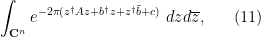
where is now a complex variable

 is the adjoint

is a complex matrix with positive definite Hermitian part,  are column vectors in , is a complex number, and
  is
is  times Lebesgue measure on . (The factors of two here turn out to be a natural normalisation, but they can be ignored on a first reading.) As we shall see later, such integrals are relevant when performing computations on the Gaussian Unitary Ensemble (GUE) in random matrix theory. Note that the integrand here is not complex analytic due to the presence of the complex conjugates. However, this can be dealt with by the trick of replacing the complex conjugate
  by a variable
  which is formally conjugate to , but which is allowed to vary independently of . More precisely, let
  be the space of all functions
  of two independent -tuples
of complex variables, which is jointly entire in all  variables (in the sense defined previously, i.e. there is a joint Taylor series that is absolutely convergent for all independent choices of
  ), and such that there is an such that for every there is such that one has the bound

whenever  . We will call such functions Schwartz analytic. Note that the integrand in (11) is Schwartz analytic when has positive definite Hermitian part, if we reinterpret as the transpose of rather than as the adjoint of in order to make the integrand entire in and . We can then define an abstract integration functional
  by the formula

thus can be localised to the slice  of
of  (though, as with previous functionals, one can use contour shifting to relocalise to other slices also.) One can also write this integral as
and note that the integrand here is a Schwartz entire function on , thus linking the Schwartz analytic integral with the Schwartz entire integral. Using this connection, one can verify that this functional is invariant with respect to translating and by independent shifts in (thus giving a translation symmetry), and one also has the independent dilation symmetry

for complex matrices  that are sufficiently close to the identity, where
  . Arguing as before, we can then compute (11) as

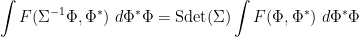
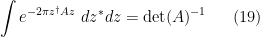
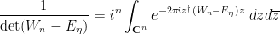
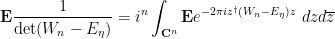
In particular, this gives an integral representation for the determinant-reciprocal  of a complex matrix with positive definite Hermitian part, in terms of gaussian expressions in which only appears linearly in the exponential:
This formula is then convenient for computing statistics such as
for random matrices  drawn from the Gaussian Unitary Ensemble (GUE), and some choice of spectral parameter
  with
with  ; we review this computation later in this post. By the trick of matrix differentiation of the determinant (as reviewed in this recent blog post), one can also use this method to compute matrix-valued statistics such as

However, if one restricts attention to classical integrals over real or complex (and in particular, commuting or bosonic) variables, it does not seem possible to easily eradicate the negative determinant factors in such calculations, which is unfortunate because many statistics of interest in random matrix theory, such as the expected Stieltjes transform

which is the Stieltjes transform of the density of states. However, it turns out (as I learned recently from Peter Sarnak and Tom Spencer) that it is possible to cancel out these negative determinant factors by balancing the bosonic gaussian integrals with an equal number of fermionic gaussian integrals, in which one integrates over a family of anticommuting variables. These fermionic integrals are closer in spirit to the polynomial integral (6) than to Lebesgue type integrals, and in particular obey a scaling law which is inverse to the Lebesgue scaling (in particular, a linear change of fermionic variables  ends up transforming a fermionic integral by
  rather than ), which conveniently cancels out the reciprocal determinants in the previous calculations. Furthermore, one can combine the bosonic and fermionic integrals into a unified integration concept, known as the Berezin integral (or Grassmann integral), in which one integrates functions of supervectors (vectors with both bosonic and fermionic components), and is of particular importance in the theory of supersymmetry in physics. (The prefix “super” in physics means, roughly speaking, that the object or concept that the prefix is attached to contains both bosonic and fermionic aspects.) When one applies this unified integration concept to gaussians, this can lead to quite compact and efficient calculations (provided that one is willing to work with “super”-analogues of various concepts in classical linear algebra, such as the supertrace or superdeterminant).
Abstract integrals of the flavour of (6) arose in quantum field theory, when physicists sought to formally compute integrals of the form

where  are familiar commuting (or bosonic) variables (which, in particular, can often be localised to be scalar variables taking values in or ), while
  were more exotic anticommuting (or fermionic) variables, taking values in some vector space of fermions. (As we shall see shortly, one can formalise these concepts by working in a supercommutative algebra.) The integrand
  was a formally analytic function of
  , in that it could be expanded as a (formal, noncommutative) power series in the variables . For functions
  that depend only on bosonic variables, it is certainly possible for such analytic functions to be in the Schwartz class and thus fall under the scope of the classical integral, as discussed previously. However, functions
  that depend on fermionic variables behave rather differently. Indeed, a fermonic variable
  must anticommute with itself, so that
  . In particular, any power series in terminates after the linear term in , so that a function
  can only be analytic in if it is a polynomial of degree at most in ; more generally, an analytic function of
  fermionic variables must be a polynomial of degree at most , and an analytic function of bosonic and fermionic variables can be Schwartz in the bosonic variables but will be polynomial in the fermonic variables. As such, to interpret the integral (14), one can use classical (Lebesgue) integration (or the variants discussed above for integrating Schwartz entire or Schwartz analytic functions) for the bosonic variables, but must use abstract integrals such as (6) for the fermonic variables, leading to the concept of Berezin integration mentioned earlier.
In this post I would like to set out some of the basic algebraic formalism of Berezin integration, particularly with regards to integration of gaussian-type expressions, and then show how this formalism can be used to perform computations involving GUE (for instance, one can compute the density of states of GUE by this machinery without recourse to the theory of orthogonal polynomials). The use of supersymmetric gaussian integrals to analyse ensembles such as GUE appears in the work of Efetov (and was also proposed in the slightly earlier works of Parisi-Sourlas and McKane, with a related approach also appearing in the work of Wegner); the material here is adapted from this survey of Mirlin, as well as the later papers of Disertori-Pinson-Spencer and of Disertori.
— 1. Grassmann algebra and Berezin integration —
Berezin integration can be performed on functions defined on the vectors in any supercommutative algebra, or even more generally on a supermanifold, but for the purposes of the applications to random matrix theory discussed here, we will only need to understand Berezin integration for analytic functions  of bosonic variables and fermionic variables.
We now set up the formal mathematical framework. We will need a space of basic fermions, which can be taken to be any infinite-dimensional abstract complex vector space. The infinite dimensionality of is convenient to avoid certain degeneracies; it may seem dangerous from an analysis perspective to integrate over such spaces, but as we will be performing integration from a purely algebraic viewpoint, this will not be a concern. (Indeed, one could avoid dealing with the individual elements of space altogether, and work instead with certain rings of functions on (thus treating as a noncommutative scheme, rather than as a set of points), but we will not adopt this viewpoint here.)
We then form the  -fold exterior powers
  , which is the universal complex vector space generated by the -fold wedge products
  of elements
  of , subject to the requirement that the wedge product
  is bilinear, and also antisymmetric on elements of . We then form the exterior algebra
 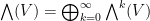 of as the direct sum of all these exterior powers. If one endows this algebra with the wedge product , one obtains a complex algebra, since the wedge product is bilinear and associative. By abuse of notation, we will write the wedge product
  simply as
  .
.
We split 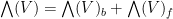 into the space
  of bosons (arising from exterior powers of even order) and the space
  of fermions (exterior powers of odd order). Thus, for instance, complex scalars (which make up
  ) are bosons, while elements of are fermions (i.e. basic fermions are fermions). We observe that the product of two bosons or two fermions is a boson, while the product of a boson and a fermion is a fermion, which gives
  the structure of a superalgebra (i.e.
  –graded algebra, with
  and
and  being the
  and graded components).
Generally speaking, we will try to use Roman symbols such as  to denote bosons, and Greek symbols such as
  to denote fermions; we will also try to use capital Greek symbols (such as
  ) to denote combinations of bosons and fermions.
It is easy to verify (as can be done for instance by using a basis  for , with the attendant basis
  ,
,  for ), that bosonic elements of are central (they commute with both bosons and fermions), while fermionic elements of commute with bosonic elements but anticommute with each other. (In other words, the superalgebra is supercommutative.)
A fermionic element will commute with all bosonic elements and anticommute with fermonic elements, which in particular implies that

One corollary of this (and the anticommutativity of with itself) is that any product in which contains two copies of will necessarily vanish. Another corollary is that all elements  in
in  are nilpotent, so that
  for some . In particular, every element in can be decomposed as the sum of a scalar and a nilpotent (in fact, this decomposition is unique). A further corollary is the fact the algebra is locally finitely dimensional, in the sense that every finite collection of elements in generates a finite dimensional subalgebra of . Among other things, this implies that every element of can be exponentiated by the usual power series
Thus, for instance, the exponential of a bosonic element is again a bosonic element, while the exponential of a fermion is just a linear function, since  anticommutes with itself and thus squares to zero:

As bosonic elements are central, we also see that we have the usual formula

whenever  is bosonic and is an arbitrary element of .
We now consider functions of bosonic variables  and fermionic variables
  . We will abbreviate
  as
as  , and write
We will restrict attention to functions  which are strongly analytic in the sense that they can be written as a strongly convergent noncommutative Taylor series in the variables with coefficients in . By strongly convergence, we mean that for any given choice of
  , all of the terms in the Taylor series lie in a finite dimensional subspace of , and the series is absolutely convergent in that finite dimensional subspace. (One could consider more relaxed notions of convergence (and thus of analyticity) here, but this strong notion of analyticity is already obeyed by the functions we will care about in applications, namely supercommutative gaussian functions with polynomial weights, so we will not need to consider more general classes of analytic functions here.)
Let  denote the space of strongly analytic functions from to . This is clearly a complex algebra, and contains all the polynomials in the variables with coefficients in , as well as exponentials of such polynomials. It is also translation invariant in all of the variables (this is a variant of the basic fact in real analysis that if a Taylor series has infinite radius of convergence at the origin, then it is also equal to a Taylor series with infinite radius of sequence at any other point). On the other hand, by collecting terms in
  for any
  , we see that any strongly analytic function can be written in the form

for some strongly analytic functions  . In fact,
  and
and  are uniquely determined from ;
  is necessarily equal to
  , and if were not unique, then on subtraction one could find an element
  with the property that
  for all
  , which is not possible because is infinite dimensional.
We then define the (one-dimensional) Berezin integral

of a strongly analytic function  with respect to the variable by the formula

the normalisation factor  is convenient for gaussian integration calculations, as we shall see later, but can be ignored for now. This is a functional from
  to
to  , which is an abstract integration functional in the sense discussed in the the introduction, because the functional is invariant with respect to translations of the variable by elements of . It also obeys the scaling law

for any invertible bosonic element  , as follows immediately from the definitions.
We can iterate the above integration operation. For instance, any can be fully decomposed in terms of the fermionic variables as

where  are strongly analytic functions of just the bosonic variables , and the sum ranges over tuples
  . We can then define the Berezin integral

of a strongly analytic function  over all the fermionic variables

at once, by the formula

This is an abstract integration functional from to  which is invariant under translations of by
  ; it can also be viewed as the iteration of the one-dimensional integrations by the Fubini-type formula

(note the reversal of the order of integration here). Much as fermions themselves anticommute with each other, one-dimensional Berezin integrals over fermonic variables also anticommute with each other, thus for instance

(compare with integration of differential forms, with  ). One also verifies the scaling law
for any invertible  matrix with bosonic entries, which can be verified for instance by first checking it in the case of diagonal matrices, permutation matrices, and shear matrices, and then observing that these generate all the other invertible matrices.
We can combine integration over fermionic variables with the more familiar integration over bosonic variables. We will focus attention on complex bosonic and fermionic integration rather than real bosonic and fermionic integration, as this will be the integration concept that is relevant for computations involving GUE. Thus, we will now consider strongly analytic functions  of bosonic variables
  and
and  fermionic variables
  . As previously discussed in the integration of Schwartz analytic functions, we allow the
  variable to vary independently of the
  variable despite being formally being denoted as an adjoint to , and similarly for
  and
and  .
.
Observe that a strongly analytic function  of purely bosonic variables will have all Taylor coefficients take values in a finite dimensional subspace
  of (otherwise it will not be strongly analytic for complex scalar non-zero
  ). In particular, if we restrict the bosonic variables to be complex scalars, then
  takes values in this subspace . We then say that is Schwartz analytic if the restriction to lies in
  , thus every component of this restriction lies in . Note that this restriction to is sufficient to recover the values of at all other values in
  , because one can read off all the Taylor coefficients of from this restriction. We denote the space of such Schwartz analytic functions as
  . We then use the functionals (12) to define Berezin integration on one or more pairs
  of bosonic variables. For instance, the Berezin integral
will, by definition, be the Lebesgue integral

recalling that  is
is  times Lebesgue measure on the complex plane in the variable, and similarly

is the quantity
One easily verifies that Berezin integration with respect to a single pair of bosonic variables maps  to
to  , and integration with respect to all the bosonic variables
  maps to .
As discussed in the introduction, a bosonic integral is invariant with respect to independent translations of the and by any complex shifts. It turns out that these integrals are in fact also invariant under independent translations of  by arbitrary bosonic shifts. For sake of notation we will just illustrate this in the
  case. From the invariance under complex shifts we have
for any complex  . But both sides of this equation are entire in both variables
  , so this identity must also hold on the level of (commutative) formal power series. Specialising from formal variables to bosonic variables we obtain the claim. For similar reasons, we have the scaling law

for all invertible matrices  with bosonic entries and scalar part sufficiently close to the identity, because the claim was already shown to be true for complex entries, and both sides are analytic in .
A function  of bosonic and fermionic variables
  and their formal adjoints
  will be called Schwartz analytic if each of its components under the decomposition (16) is Schwartz analytic, and the space of such functions will be denoted
  . One can then perform Berezin integration with respect to a pair
  of bosonic variables by integrating each term in (16) separately; this creates an integration functional from to
  . Similarly, one can integrate out all the bosonic variables at once, creating an integration functional from to
  . Meanwhile, fermionic integration in a pair
  maps can be verified to map to
  , and integrating out all pairs at once leads to a functional from to
  . Finally, one can check that bosonic integration commutes with either fermionic and bosonic integration, and fermionic integration anticommutes with fermionic integration; in particular, integrating a pair of is an operation that commutes with other such operations or with bosonic integration. Because of this, one can now define the full Berezin integral

of a Schwartz analytic function  by integrating out all the pairs and (with the order in which these pairs are integrated being irrelevant). This gives an integration functional from to . From the translation invariance properties of the individual bosonic and fermonic integrals, we see that this functional is invariant with respect to independent translations of and
  by elements of .
Example 1 Take  . If
. If  are bosons with the real scalar part of being positive, then the gaussian function
can be expanded (using the nilpotent nature of  ) as
) as
or equivalently

and this is a Schwartz analytic function on  . Performing the bosonic integrals (using (13)) we then get
and then on performing the fermionic integrals we obtain
If instead one performs the fermionic integral first, one obtains

and then on performing the bosonic integrals one ends up at the same place:

Note how the parameters and scale in the opposite way in this integral.
We now derive the general scaling law for Berezin integrals

in which we scale by a matrix that suitably respects the bosonic and fermonic components of . More precisely, define an  supermatrix to be a
  block matrix of the form

where  is a matrix with bosonic entries,
  is an
is an  matrix with fermionic entries,
  is an
is an  matrix with fermionic entries, and
  is an matrix with bosonic entries. Observe that if is an
  -dimensional column supervector and
  is an -dimensional row supervector then

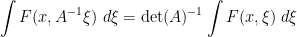
Proposition 1 (Scaling law) Let  be a Schwartz analytic function, and let
  be a matrix. If the scalar part of is sufficiently close to the identity (or equivalently, the scalar parts of are sufficiently close to the identity), then we have
where  is the superdeterminant (also known as the Berezinian) of , defined by the formula

(in particular, this quantity is bosonic).
The formula for the superdeterminant should be compared with the Schur complement formula
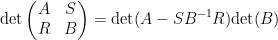
for ordinary block matrices (which was discussed in this previous blog post)
Proof: When is a block-diagonal matrix (so that  and
and  vanish, and the superdeterminant simplifies to
  ), the claim follows from the separate scaling laws for bosonic and fermonic integration obtained previously. When is a shear matrix (so that and
  are the identity, and one of
  vanishes, and the superdeterminant simplifies to ) the claim follows from the translation invariance of either the fermonic or bosonic integral (after performing these two integrals in a suitable order). For the general case, we use the factorisation

noting that the two shear matrices have superdeterminant , while the block-diagonal matrix has the same superdeterminant as , to deduce the general case from the two special cases previously mentioned. 
One consequence of this scaling law (and the nontrivial nature of the Berezin integral) is that one has the mutliplication law

for any two supermatrices  , at least if their scalar parts are sufficiently close to the identity. This in turn implies that the superdeterminant is the multiplicative analogue of the supertrace
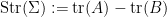
in the sense that

for any supermatrix (at least if its scalar part is sufficiently small). Note also that the supertrace obeys the expected cyclic property
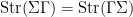
which can also be deduced from the previous identities by matrix differentiation, as indicated in this previous post.
By repeating the derivation of (13) (reducing to integrals that are basically higher dimensional versions of Example 1), one has the Grassmann gaussian integral formula

whenever is an supermatrix whose bosonic part  has positive definite scalar Hermitian part,
  are -dimensional supervectors, and , with being the transpose of . In particular, one has

We can isolate the bosonic and fermionic special cases of this identity, namely
and
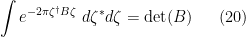
whenever , are and matrices with bosonic entries respectively. For comparison, we also observe the real fermionic analogue of these identities, namely
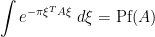
where the Berezin integral is now over fermonic variables , and is an antisymmetric bosonic matrix, with  being the Pfaffian of . This can be seen by directly Taylor expanding
  and isolating the
  term. One can then develop a theory of superpfaffians in analogy to that of superdeterminants, which among other things may be helpful for manipulating the Gaussian Orthogonal Ensemble (GOE) (or at least the skew-symmetric analogue of GOE), but we will not do so here.
As noted in this previous blog post, one can often start with an identity involving a determinant and apply matrix differentiation to obtain further useful identities. If we start with (18), replace by an infinitesimal perturbation  for an arbitrary supermatrix
  matrix, and extract the linear component in , one arrives at the identity

In particular, if we set to be the elementary matrix
then we have
and in particular (if we have no fermionic elements)

— 2. Application to GUE statistics —
We now use the above Gaussian integral identities to compute some GUE statistics. These statistics are initially rather complicated looking integrals over  variables, but after some application of the above identities, we can cut the number of variables of integration down to
  , and by a further use of these gaussian identities we can reduce this number down to just
  , at which point it becomes feasible to obtain asympotics for such integrals by techniques such as the method of steepest descent (also known as the saddle point method).
To illustrate this general phenomenon, we begin with a simple example which only requires classical (or bosonic) integration.
Proposition 2 Let be a GUE matrix, thus 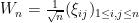 where
where  has the standard real normal distribution
  (i.e. density function
  ) when
  , and the standard complex normal distribution
  (i.e. density function
  ) when
  , with being jointly independent for
  . Let
. Let  be a complex number with positive imaginary part
  . Then

Proof: From (19) (or (13)) applied to  (which has Hermitian part ) we have
and so by Fubini’s theorem (which can be easily justified in view of all the exponential decay in the integrand) we have
Now observe that the top left  coordinate of is
  , and
, and  has the standard normal distribution
  . Thus we have


for any  with non-negative real part, thanks to (9). By the unitary invariance of the GUE ensemble , we thus have

since we can use that invariance to reduce to the case  , and the claim follows.
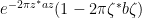
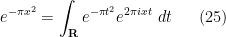
The right-hand side of (23) is simpler than the left-hand side, as the integration is only over (as opposed to the  -dimensional space of Hermitian matrices), and there are no determinant factors. The integral can be simplified further by the following trick (known to physicists as the Hubbard-Stratonovich transformation. As the gaussian
  is its own Fourier transform, we have
for any  (and also for
  , by analytic continuation). The point here is that a quadratic exponential in can be replaced with a combination of linear exponentials in . Applying this identity with replaced by
  , we conclude that

thus replacing a quartic exponential by a combination of quadratic ones. By Fubini’s theorem, the right-hand side of (23) can be written
Applying (10) one has

and so (23) simplifies further to
We thus see that the expression  has now been reduced to a one-dimensional integral, which can be estimated by a variety of techniques, such as the method of steepest descent (also known as the saddle point method).
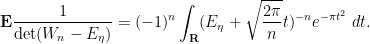
The equation (22) allows one to manipulate components of an inverse  of a matrix, so long as this component is weighted by a reciprocal determinant. For instance, it implies that

for any  , and so by repeating the proof of Proposition 2 one has


We can use (26) to write the above expression as

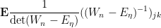
By (22) one has
where  is the Kronecker delta function. We thus have
By introducing fermionic variables  and their formal adjoints
  , one can now eliminate the reciprocal determinant. Indeed, from (20) one has

combining this with (27) one has

where consists of bosonic and fermionic variables, and we have abused notation by identifying the matrix  with the supermatrix
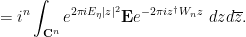
Now we compute the expectation

It is convenient here to realise the Wigner ensemble as the Hermitian part  of a complex gaussian matrix (with entries being iid copies of ). Then the above expression is
where  is a suitable Haar measure on the space of complex matrices, normalised so that

We can expand this as
and rearrange this as

By contour shifting  and
and  separately, we see that the integral here is still . One can also compute that

and so we can write
as

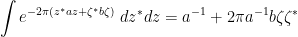
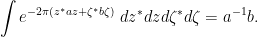
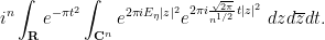
To simplify this -dimensional integral, we use the Hubbard-Stratonovich transformation. From (25) (which can be extended by analyticity from complex to hosonic ) we have
and

while from (17) (with  ,
,  ,
,  ,
,  , and
, and  ) one has

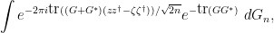
and so the expression (30) becomes

where  is the
  supermatrix
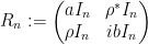
and  is the identity matrix.
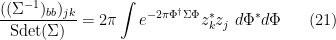
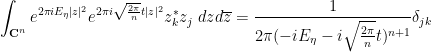
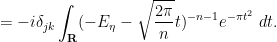
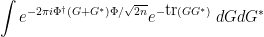
One can perform the  integrals using (21), yielding
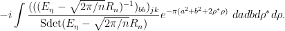
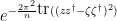
This expression may look somewhat complicated, but there are now only four variables of integration (two bosonic and two fermionic), and this can be evaluated exactly by a tedious but straightforward computation; see this paper of Disertori for details. After evaluating the fermionic integrals and performing some rescalings, one eventually arrives at the exact expression

for (29), which can then be estimated by a (somewhat involved) application of the method of steepest descent; again, see the paper of Disertori for details.


15 comments
Comments feed for this article
20 February, 2013 at 2:54 am
La derivación y la integración desde un punto de vista algebraico « Adsu's Blog
[…] un reblog de nuestro crack Terry Tao sobre como capturar los conceptos esenciales de la derivación y la […]
20 February, 2013 at 5:24 am
humberto triviño
el crearlos en ocasiones podría restringir ciertos aspectos que son inherentes en el mismo espacio, aunque facilite ciertos procesos .
entiendo la conexión, pero me asalta la duda del manejos de este tipo de invariantes
20 February, 2013 at 8:32 am
Jon Awbrey
Puzzle Question. Over GF(2) minus and plus are the same. What does this mean for the theories of differentiation and integration over GF(2)?
Cf. Links to differential logic papers on this bib page.
20 February, 2013 at 4:17 pm
dochunosei
Nice post. I have a couple of points/questions, mostly directed at the issue of renormalization for formal integration of polynomials. First, one could make polynomials genuinely integrable by integrating against, say, $e^{-x^2} d x$. This would mean sacrificing translation invariance, but can anything be salvaged from which one could build a corresponding formal algebraic integral? Second, in view of Remark 1 and the application in Sec. 1, is there a connection between the notion of renormalization used here and renormalization groups as used in quantum field theory and statistical mechanics?
21 February, 2013 at 7:29 pm
Terence Tao
When weighted against, say, , the analogue of the condition
  in the above post is now
  . It is then again true that functionals that obey this law and obey some mild regularity conditions must come from integration against some constant multiple of
  ; this observation, incidentally, serves as motivation for Stein’s method in probability.
As for the renormalisation here, it is quite a simple one (extracting a mean value of a function at a very large scale) and is not really on the same level of sophistication as renormalisation group theory which deals with self-similarity across multiple scales.
21 February, 2013 at 6:16 am
Kasper Henriksen
But in (4) you have that {I(x\mapsto \exp(-\pi x^2))=1}, so {I} can’t annihilate all mean zero Schwartz functions?
21 February, 2013 at 6:20 am
dochunosei
An unfortunate confusion of terminology: that Gaussian bump has its centre of mass (i.e. the integral of ) at 0, but its total mass (i.e. the integral
  ) is 1. I think that when Prof. Tao wrote “mean zero” he meant “total mass = 0”, not “centre of mass = 0”.
[Reworded to reduce confusion – T.]
21 February, 2013 at 2:50 pm
Alexander Shamov
When you talk of “bosonic and fermionic quantities”, do you actually mean that we should leave the freedom to consider supercommutative extensions of the ring of scalars itself?
21 February, 2013 at 2:57 pm
Alexander Shamov
Ah, sorry, I overlooked that your functions were -valued in the first place…
28 February, 2013 at 8:45 pm
Qiaochu Yuan
Is anyone else having trouble with the RSS feed for these posts? This post still hasn’t shown up in my feed.
16 March, 2013 at 1:20 pm
Jérôme Chauvet
Hi Terrence,
The terminology ” supercommutative algebra” sounds weird. The link to wikipedia you provided deals with -graded algebra, which Alain Connes used in “non commutative geometry” – you can check for instance http://www.alainconnes.org/docs/book94bigpdf.pdf (page 445). Do we then use supercommutaive algebra for solving noncommutative geometry problems? Rather confusing…
Thanx
17 March, 2013 at 2:13 am
Jérôme Chauvet
Hi Terry,
Remark 1 : Error writing the formula of a polynomial.
Best reagrds,
[Corrected, thanks – T.]
18 March, 2013 at 1:38 pm
Jérôme Chauvet
Error in Remark 1 still there however.
I guess should be corrected to
  .
.
[Oops, that should be fixed now – T.]
29 June, 2019 at 3:13 pm
Symmetric functions in a fractional number of variables, and the multilinear Kakeya conjecture | What's new
[…] in the physical literature in order to assign values to otherwise divergent integrals. See also this post for an unrelated abstraction of the integration concept involving integration over supercommutative […]
6 February, 2023 at 1:46 pm
Edward
I think there’s a typo in the definition of the (one-dimensional) Berezin integral of a strongly analytic function w/r/t the variable. The RHS shouldn’t be an integral.
[Corrected, thanks – T.]