Notes on the B+B+t theorem

A recent paper of Kra, Moreira, Richter, and Robertson established the following theorem, resolving a question of Erdös. Given a discrete amenable group , and a subset of , we define the Banach density of to be the quantity

where the supremum is over all Følner sequences of . Given a set in , we define the restricted sumset to be the set of all pairs where are distinct elements of .

Theorem 1 Let be a countably infinite abelian group with the index finite. Let be a positive Banach density subset of . Then there exists an infinite set and such that .

Strictly speaking, the main result of Kra et al. only claims this theorem for the case of the integers , but as noted in the recent preprint of Charamaras and Mountakis, the argument in fact applies for all countable abelian in which the subgroup has finite index. This condition is in fact necessary (as observed by forthcoming work of Ethan Acklesberg): if has infinite index, then one can find a subgroup of of index for any that contains (or equivalently, is -torsion). If one lets be an enumeration of , and one can then check that the set

has positive Banach density, but does not contain any set of the form for any (indeed, from the pigeonhole principle and the -torsion nature of one can show that must intersect whenever has cardinality larger than ). It is also necessary to work with restricted sums rather than full sums : a counterexample to the latter is provided for instance by the example with and . Finally, the presence of the shift is also necessary, as can be seen by considering the example of being the odd numbers in , though in the case one can of course delete the shift at the cost of giving up the containment .

Theorem 1 resembles other theorems in density Ramsey theory, such as Szemerédi’s theorem, but with the notable difference that the pattern located in the dense set is infinite rather than merely arbitrarily large but finite. As such, it does not seem that this theorem can be proven by purely finitary means. However, one can view this result as the conjunction of an infinite number of statements, each of which is a finitary density Ramsey theory statement. To see this, we need some more notation. Observe from Tychonoff’s theorem that the collection is a compact topological space (with the topology of pointwise convergence) (it is also metrizable since is countable). Subsets of can be thought of as properties of subsets of ; for instance, the property a subset of of being finite is of this form, as is the complementary property of being infinite. A property of subsets of can then be said to be closed or open if it corresponds to a closed or open subset of . Thus, a property is closed and only if if it is closed under pointwise limits, and a property is open if, whenever a set has this property, then any other set that shares a sufficiently large (but finite) initial segment with will also have this property. Since is compact and Hausdorff, a property is closed if and only if it is compact.

The properties of being finite or infinite are neither closed nor open. Define a smallness property to be a closed (or compact) property of subsets of that is only satisfied by finite sets; the complement to this is a largeness property, which is an open property of subsets of that is satisfied by all infinite sets. (One could also choose to impose other axioms on these properties, for instance requiring a largeness property to be an upper set, but we will not do so here.) Examples of largeness properties for a subset of include:

• has at least elements.
• is non-empty and has at least elements, where is the smallest element of .
• is non-empty and has at least elements, where is the element of .
• halts when given as input, where is a given Turing machine that halts whenever given an infinite set as input. (Note that this encompasses the preceding three examples as special cases, by selecting appropriately.)

We will call a set obeying a largeness property an -large set.

Theorem 1 is then equivalent to the following “almost finitary” version (cf. this previous discussion of almost finitary versions of the infinite pigeonhole principle):

Theorem 2 (Almost finitary form of main theorem) Let be a countably infinite abelian group with finite. Let be a Følner sequence in , let , and let be a largeness property for each . Then there exists such that if is such that for all , then there exists a shift and contains a -large set such that .

Proof of Theorem 2 assuming Theorem 1. Let , , be as in Theorem 2. Suppose for contradiction that Theorem 2 failed, then for each we can find with for all , such that there is no and -large such that . By compactness, a subsequence of the converges pointwise to a set , which then has Banach density at least . By Theorem 1, there is an infinite set and a such that . By openness, we conclude that there exists a finite -large set contained in , thus . This implies that for infinitely many , a contradiction.

Proof of Theorem 1 assuming Theorem 2. Let be as in Theorem 1. If the claim failed, then for each , the property of being a set for which would be a smallness property. By Theorem 2, we see that there is a and a obeying the complement of this property such that , a contradiction.

Remark 3 Define a relation between and by declaring if and . The key observation that makes the above equivalences work is that this relation is continuous in the sense that if is an open subset of , then the inverse image

is also open. Indeed, if for some , then contains a finite set such that , and then any that contains both and lies in .

For each specific largeness property, such as the examples listed previously, Theorem 2 can be viewed as a finitary assertion (at least if the property is “computable” in some sense), but if one quantifies over all largeness properties, then the theorem becomes infinitary. In the spirit of the Paris-Harrington theorem, I would in fact expect some cases of Theorem 2 to undecidable statements of Peano arithmetic, although I do not have a rigorous proof of this assertion.

Despite the complicated finitary interpretation of this theorem, I was still interested in trying to write the proof of Theorem 1 in some sort of “pseudo-finitary” manner, in which one can see analogies with finitary arguments in additive combinatorics. The proof of Theorem 1 that I give below the fold is my attempt to achieve this, although to avoid a complete explosion of “epsilon management” I will still use at one juncture an ergodic theory reduction from the original paper of Kra et al. that relies on such infinitary tools as the ergodic decomposition, the ergodic theory, and the spectral theorem. Also some of the steps will be a little sketchy, and assume some familiarity with additive combinatorics tools (such as the arithmetic regularity lemma).

A generalized Cauchy-Schwarz inequality via the Gibbs variational formula

Let be a non-empty finite set. If is a random variable taking values in , the Shannon entropy of is defined as

There is a nice variational formula that lets one compute logs of sums of exponentials in terms of this entropy:

Lemma 1 (Gibbs variational formula) Let be a function. Then

Proof: Note that shifting by a constant affects both sides of (1) the same way, so we may normalize . Then is now the probability distribution of some random variable , and the inequality can be rewritten as

But this is precisely the Gibbs inequality. (The expression inside the supremum can also be written as , where denotes Kullback-Leibler divergence. One can also interpret this inequality as a special case of the Fenchel–Young inequality relating the conjugate convex functions and .)

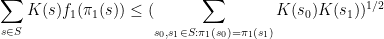
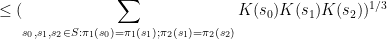
In this note I would like to use this variational formula (which is also known as the Donsker-Varadhan variational formula) to give another proof of the following inequality of Carbery.

Theorem 2 (Generalized Cauchy-Schwarz inequality) Let , let be finite non-empty sets, and let be functions for each . Let and be positive functions for each . Then

where is the quantity

where is the set of all tuples such that for .

Thus for instance, the identity is trivial for . When , the inequality reads

which is easily proven by Cauchy-Schwarz, while for the inequality reads

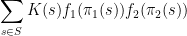
which can also be proven by elementary means. However even for , the existing proofs require the “tensor power trick” in order to reduce to the case when the are step functions (in which case the inequality can be proven elementarily, as discussed in the above paper of Carbery).

We now prove this inequality. We write and for some functions and . If we take logarithms in the inequality to be proven and apply Lemma 1, the inequality becomes

where ranges over random variables taking values in , range over tuples of random variables taking values in , and range over random variables taking values in . Comparing the suprema, the claim now reduces to

Lemma 3 (Conditional expectation computation) Let be an -valued random variable. Then there exists a -valued random variable , where each has the same distribution as , and

Proof: We induct on . When we just take . Now suppose that , and the claim has already been proven for , thus one has already obtained a tuple with each having the same distribution as , and

By hypothesis, has the same distribution as . For each value attained by , we can take conditionally independent copies of and conditioned to the events and respectively, and then concatenate them to form a tuple in , with a further copy of that is conditionally independent of relative to . One can the use the entropy chain rule to compute

and the claim now follows from the induction hypothesis.

With a little more effort, one can replace by a more general measure space (and use differential entropy in place of Shannon entropy), to recover Carbery’s inequality in full generality; we leave the details to the interested reader.

A slightly longer Lean 4 proof tour

In my previous post, I walked through the task of formally deducing one lemma from another in Lean 4. The deduction was deliberately chosen to be short and only showcased a small number of Lean tactics. Here I would like to walk through the process I used for a slightly longer proof I worked out recently, after seeing the following challenge from Damek Davis: to formalize (in a civilized fashion) the proof of the following lemma:

Lemma. Let and be sequences of real numbers indexed by natural numbers , with non-increasing and non-negative. Suppose also that for all . Then for all .

Here I tried to draw upon the lessons I had learned from the PFR formalization project, and to first set up a human readable proof of the lemma before starting the Lean formalization – a lower-case “blueprint” rather than the fancier Blueprint used in the PFR project. The main idea of the proof here is to use the telescoping series identity

Since is non-negative, and by hypothesis, we have

but by the monotone hypothesis on the left-hand side is at least , giving the claim.

This is already a human-readable proof, but in order to formalize it more easily in Lean, I decided to rewrite it as a chain of inequalities, starting at and ending at . With a little bit of pen and paper effort, I obtained

(by field identities)

(by the formula for summing a constant)

(by the monotone hypothesis)

(by the hypothesis

(by telescoping series)

(by the non-negativity of ).

I decided that this was a good enough blueprint for me to work with. The next step is to formalize the statement of the lemma in Lean. For this quick project, it was convenient to use the online Lean playground, rather than my local IDE, so the screenshots will look a little different from those in the previous post. (If you like, you can follow this tour in that playground, by clicking on the screenshots of the Lean code.) I start by importing Lean’s math library, and starting an example of a statement to state and prove:

Now we have to declare the hypotheses and variables. The main variables here are the sequences and , which in Lean are best modeled by functions a, D from the natural numbers ℕ to the reals ℝ. (One can choose to “hardwire” the non-negativity hypothesis into the by making D take values in the nonnegative reals (denoted NNReal in Lean), but this turns out to be inconvenient, because the laws of algebra and summation that we will need are clunkier on the non-negative reals (which are not even a group) than on the reals (which are a field). So we add in the variables:

Now we add in the hypotheses, which in Lean convention are usually given names starting with h. This is fairly straightforward; the one thing is that the property of being monotone decreasing already has a name in Lean’s Mathlib, namely Antitone, and it is generally a good idea to use the Mathlib provided terminology (because that library contains a lot of useful lemmas about such terms).

One thing to note here is that Lean is quite good at filling in implied ranges of variables. Because a and D have the natural numbers ℕ as their domain, the dummy variable k in these hypotheses is automatically being quantified over ℕ. We could have made this quantification explicit if we so chose, for instance using ∀ k : ℕ, 0 ≤ D k instead of ∀ k, 0 ≤ D k, but it is not necessary to do so. Also note that Lean does not require parentheses when applying functions: we write D k here rather than D(k) (which in fact does not compile in Lean unless one puts a space between the D and the parentheses). This is slightly different from standard mathematical notation, but is not too difficult to get used to.

This looks like the end of the hypotheses, so we could now add a colon to move to the conclusion, and then add that conclusion:

This is a perfectly fine Lean statement. But it turns out that when proving a universally quantified statement such as ∀ k, a k ≤ D 0 / (k + 1), the first step is almost always to open up the quantifier to introduce the variable k (using the Lean command intro k). Because of this, it is slightly more efficient to hide the universal quantifier by placing the variable k in the hypotheses, rather than in the quantifier (in which case we have to now specify that it is a natural number, as Lean can no longer deduce this from context):

At this point Lean is complaining of an unexpected end of input: the example has been stated, but not proved. We will temporarily mollify Lean by adding a sorry as the purported proof:

Now Lean is content, other than giving a warning (as indicated by the yellow squiggle under the example) that the proof contains a sorry.

It is now time to follow the blueprint. The Lean tactic for proving an inequality via chains of other inequalities is known as calc. We use the blueprint to fill in the calc that we want, leaving the justifications of each step as “sorry”s for now:

Here, we “open“ed the Finset namespace in order to easily access Finset‘s range function, with range k basically being the finite set of natural numbers , and also “open“ed the BigOperators namespace to access the familiar ∑ notation for (finite) summation, in order to make the steps in the Lean code resemble the blueprint as much as possible. One could avoid opening these namespaces, but then expressions such as ∑ i in range (k+1), a i would instead have to be written as something like Finset.sum (Finset.range (k+1)) (fun i ↦ a i), which looks a lot less like like standard mathematical writing. The proof structure here may remind some readers of the “two column proofs” that are somewhat popular in American high school geometry classes.

Now we have six sorries to fill. Navigating to the first sorry, Lean tells us the ambient hypotheses, and the goal that we need to prove to fill that sorry:

The ⊢ symbol here is Lean’s marker for the goal. The uparrows ↑ are coercion symbols, indicating that the natural number k has to be converted to a real number in order to interact via arithmetic operations with other real numbers such as a k, but we can ignore these coercions for this tour (for this proof, it turns out Lean will basically manage them automatically without need for any explicit intervention by a human).

The goal here is a self-evident algebraic identity; it involves division, so one has to check that the denominator is non-zero, but this is self-evident. In Lean, a convenient way to establish algebraic identities is to use the tactic field_simp to clear denominators, and then ring to verify any identity that is valid for commutative rings. This works, and clears the first sorry:

field_simp, by the way, is smart enough to deduce on its own that the denominator k+1 here is manifestly non-zero (and in fact positive); no human intervention is required to point this out. Similarly for other “clearing denominator” steps that we will encounter in the other parts of the proof.

Now we navigate to the next `sorry`. Lean tells us the hypotheses and goals:

We can reduce the goal by canceling out the common denominator ↑k+1. Here we can use the handy Lean tactic congr, which tries to match two sides of an equality goal as much as possible, and leave any remaining discrepancies between the two sides as further goals to be proven. Applying congr, the goal reduces to

Here one might imagine that this is something that one can prove by induction. But this particular sort of identity – summing a constant over a finite set – is already covered by Mathlib. Indeed, searching for Finset, sum, and const soon leads us to the Finset.sum_const lemma here. But there is an even more convenient path to take here, which is to apply the powerful tactic simp, which tries to simplify the goal as much as possible using all the “simp lemmas” Mathlib has to offer (of which Finset.sum_const is an example, but there are thousands of others). As it turns out, simp completely kills off this identity, without any further human intervention:

Now we move on to the next sorry, and look at our goal:

congr doesn’t work here because we have an inequality instead of an equality, but there is a powerful relative gcongr of congr that is perfectly suited for inequalities. It can also open up sums, products, and integrals, reducing global inequalities between such quantities into pointwise inequalities. If we invoke gcongr with i hi (where we tell gcongr to use i for the variable opened up, and hi for the constraint this variable will satisfy), we arrive at a greatly simplified goal (and a new ambient variable and hypothesis):

Now we need to use the monotonicity hypothesis on a, which we have named ha here. Looking at the documentation for Antitone, one finds a lemma that looks applicable here:

One can apply this lemma in this case by writing apply Antitone.imp ha, but because ha is already of type Antitone, we can abbreviate this to apply ha.imp. (Actually, as indicated in the documentation, due to the way Antitone is defined, we can even just use apply ha here.) This reduces the goal nicely:

The goal is now very close to the hypothesis hi. One could now look up the documentation for Finset.range to see how to unpack hi, but as before simp can do this for us. Invoking simp at hi, we obtain

Now the goal and hypothesis are very close indeed. Here we can just close the goal using the linarith tactic used in the previous tour:

The next sorry can be resolved by similar methods, using the hypothesis hD applied at the variable i:

Now for the penultimate sorry. As in a previous step, we can use congr to remove the denominator, leaving us in this state:

This is a telescoping series identity. One could try to prove it by induction, or one could try to see if this identity is already in Mathlib. Searching for Finset, sum, and sub will locate the right tool (as the fifth hit), but a simpler way to proceed here is to use the exact? tactic we saw in the previous tour:

A brief check of the documentation for sum_range_sub' confirms that this is what we want. Actually we can just use apply sum_range_sub' here, as the apply tactic is smart enough to fill in the missing arguments:

One last sorry to go. As before, we use gcongr to cancel denominators, leaving us with

This looks easy, because the hypothesis hpos will tell us that D (k+1) is nonnegative; specifically, the instance hpos (k+1) of that hypothesis will state exactly this. The linarith tactic will then resolve this goal once it is told about this particular instance:

We now have a complete proof – no more yellow squiggly line in the example. There are two warnings though – there are two variables i and hi introduced in the proof that Lean’s “linter” has noticed are not actually used in the proof. So we can rename them with underscores to tell Lean that we are okay with them not being used:

This is a perfectly fine proof, but upon noticing that many of the steps are similar to each other, one can do a bit of “code golf” as in the previous tour to compactify the proof a bit:

With enough familiarity with the Lean language, this proof actually tracks quite closely with (an optimized version of) the human blueprint.

This concludes the tour of a lengthier Lean proving exercise. I am finding the pre-planning step of the proof (using an informal “blueprint” to break the proof down into extremely granular pieces) to make the formalization process significantly easier than in the past (when I often adopted a sequential process of writing one line of code at a time without first sketching out a skeleton of the argument). (The proof here took only about 15 minutes to create initially, although for this blog post I had to recreate it with screenshots and supporting links, which took significantly more time.) I believe that a realistic near-term goal for AI is to be able to fill in automatically a significant fraction of the sorts of atomic “sorry“s of the size one saw in this proof, allowing one to convert a blueprint to a formal Lean proof even more rapidly.

One final remark: in this tour I filled in the “sorry“s in the order in which they appeared, but there is actually no requirement that one does this, and once one has used a blueprint to atomize a proof into self-contained smaller pieces, one can fill them in in any order. Importantly for a group project, these micro-tasks can be parallelized, with different contributors claiming whichever “sorry” they feel they are qualified to solve, and working independently of each other. (And, because Lean can automatically verify if their proof is correct, there is no need to have a pre-existing bond of trust with these contributors in order to accept their contributions.) Furthermore, because the specification of a “sorry” someone can make a meaningful contribution to the proof by working on an extremely localized component of it without needing the mathematical expertise to understand the global argument. This is not particularly important in this simple case, where the entire lemma is not too hard to understand to a trained mathematician, but can become quite relevant for complex formalization projects.

Formalizing the proof of PFR in Lean4 using Blueprint: a short tour

Since the release of my preprint with Tim, Ben, and Freddie proving the Polynomial Freiman-Ruzsa (PFR) conjecture over , I (together with Yael Dillies and Bhavik Mehta) have started a collaborative project to formalize this argument in the proof assistant language Lean4. It has been less than a week since the project was launched, but it is proceeding quite well, with a significant fraction of the paper already either fully or partially formalized. The project has been greatly assisted by the Blueprint tool of Patrick Massot, which allows one to write a human-readable “blueprint” of the proof that is linked to the Lean formalization; similar blueprints have been used for other projects, such as Scholze’s liquid tensor experiment. For the PFR project, the blueprint can be found here. One feature of the blueprint that I find particularly appealing is the dependency graph that is automatically generated from the blueprint, and can provide a rough snapshot of how far along the formalization has advanced. For PFR, the latest state of the dependency graph can be found here. At the current time of writing, the graph looks like this:

The color coding of the various bubbles (for lemmas) and rectangles (for definitions) is explained in the legend to the dependency graph, but roughly speaking the green bubbles/rectangles represent lemmas or definitions that have been fully formalized, and the blue ones represent lemmas or definitions which are ready to be formalized (their statements, but not proofs, have already been formalized, as well as those of all prerequisite lemmas and proofs). The goal is to get all the bubbles leading up to and including the “pfr” bubble at the bottom colored in green.

In this post I would like to give a quick “tour” of the project, to give a sense of how it operates. If one clicks on the “pfr” bubble at the bottom of the dependency graph, we get the following:

Here, Blueprint is displaying a human-readable form of the PFR statement. This is coming from the corresponding portion of the blueprint, which also comes with a human-readable proof of this statement that relies on other statements in the project:

(I have cropped out the second half of the proof here, as it is not relevant to the discussion.)

Observe that the “pfr” bubble is white, but has a green border. This means that the statement of PFR has been formalized in Lean, but not the proof; and the proof itself is not ready to be formalized, because some of the prerequisites (in particular, “entropy-pfr” (Theorem 6.16)) do not even have their statements formalized yet. If we click on the “Lean” link below the description of PFR in the dependency graph, we are lead to the (auto-generated) Lean documentation for this assertion:

This is what a typical theorem in Lean looks like (after a procedure known as “pretty printing”). There are a number of hypotheses stated before the colon, for instance that is a finite elementary abelian group of order (this is how we have chosen to formalize the finite field vector spaces ), that is a non-empty subset of (the hypothesis that is non-empty was not stated in the LaTeX version of the conjecture, but we realized it was necessary in the formalization, and will update the LaTeX blueprint shortly to reflect this) with the cardinality of less than times the cardinality of , and the statement after the colon is the conclusion: that can be contained in the sum of a subgroup of and a set of cardinality at most .

The astute reader may notice that the above theorem seems to be missing one or two details, for instance it does not explicitly assert that is a subgroup. This is because the “pretty printing” suppresses some of the information in the actual statement of the theorem, which can be seen by clicking on the “Source” link:

Here we see that is required to have the “type” of an additive subgroup of . (Lean’s language revolves very strongly around types, but for this tour we will not go into detail into what a type is exactly.) The prominent “sorry” at the bottom of this theorem asserts that a proof is not yet provided for this theorem, but the intention of course is to replace this “sorry” with an actual proof eventually.

Filling in this “sorry” is too hard to do right now, so let’s look for a simpler task to accomplish instead. Here is a simple intermediate lemma “ruzsa-nonneg” that shows up in the proof:

The expression refers to something called the entropic Ruzsa distance between and , which is something that is defined elsewhere in the project, but for the current discussion it is not important to know its precise definition, other than that it is a real number. The bubble is blue with a green border, which means that the statement has been formalized, and the proof is ready to be formalized also. The blueprint dependency graph indicates that this lemma can be deduced from just one preceding lemma, called “ruzsa-diff“:

“ruzsa-diff” is also blue and bordered in green, so it has the same current status as “ruzsa-nonneg“: the statement is formalized, and the proof is ready to be formalized also, but the proof has not been written in Lean yet. The quantity , by the way, refers to the Shannon entropy of , defined elsewhere in the project, but for this discussion we do not need to know its definition, other than to know that it is a real number.

Looking at Lemma 3.11 and Lemma 3.13 it is clear how the former will imply the latter: the quantity is clearly non-negative! (There is a factor of present in Lemma 3.11, but it can be easily canceled out.) So it should be an easy task to fill in the proof of Lemma 3.13 assuming Lemma 3.11, even if we still don’t know how to prove Lemma 3.11 yet. Let’s first look at the Lean code for each lemma. Lemma 3.11 is formalized as follows:

Again we have a “sorry” to indicate that this lemma does not currently have a proof. The Lean notation (as well as the name of the lemma) differs a little from the LaTeX version for technical reasons that we will not go into here. (Also, the variables are introduced at an earlier stage in the Lean file; again, we will ignore this point for the ensuing discussion.) Meanwhile, Lemma 3.13 is currently formalized as

OK, I’m now going to try to fill in the latter “sorry”. In my local copy of the PFR github repository, I open up the relevant Lean file in my editor (Visual Studio Code, with the lean4 extension) and navigate to the “sorry” of “rdist_nonneg”. The accompanying “Lean infoview” then shows the current state of the Lean proof:

Here we see a number of ambient hypotheses (e.g., that is an additive commutative group, that is a map from to , and so forth; many of these hypotheses are not actually relevant for this particular lemma), and at the bottom we see the goal we wish to prove.

OK, so now I’ll try to prove the claim. This is accomplished by applying a series of “tactics” to transform the goal and/or hypotheses. The first step I’ll do is to put in the factor of that is needed to apply Lemma 3.11. This I will do with the “suffices” tactic, writing in the proof

I now have two goals (and two “sorries”): one to show that implies , and the other to show that . (The yellow squiggly underline indicates that this lemma has not been fully proven yet due to the presence of “sorry”s. The dot “.” is a syntactic marker that is useful to separate the two goals from each other, but you can ignore it for this tour.) The Lean tactic “suffices” corresponds, roughly speaking, to the phrase “It suffices to show that …” (or more precisely, “It suffices to show that … . To see this, … . It remains to verify the claim …”) in Mathematical English. For my own education, I wrote a “Lean phrasebook” of further correspondences between lines of Lean code and sentences or phrases in Mathematical English, which can be found here.

Let’s fill in the first “sorry”. The tactic state now looks like this (cropping out some irrelevant hypotheses):

Here I can use a handy tactic “linarith“, which solves any goal that can be derived by linear arithmetic from existing hypotheses:

This works, and now the tactic state reports no goals left to prove on this branch, so we move on to the remaining sorry, in which the goal is now to prove :

Here we will try to invoke Lemma 3.11. I add the following lines of code:

The Lean tactic “have” roughly corresponds to the Mathematical English phrase “We have the statement…” or “We claim the statement…”; like “suffices”, it splits a goal into two subgoals, though in the reversed order to “suffices”.

I again have two subgoals, one to prove the bound (which I will call “h”), and then to deduce the previous goal from . For the first, I know I should invoke the lemma “diff_ent_le_rdist” that is encoding Lemma 3.11. One way to do this is to try the tactic “exact?”, which will automatically search to see if the goal can already be deduced immediately from an existing lemma. It reports:

So I try this (by clicking on the suggested code, which automatically pastes it into the right location), and it works, leaving me with the final “sorry”:

The lean tactic “exact” corresponds, roughly speaking, to the Mathematical English phrase “But this is exactly …”.

At this point I should mention that I also have the Github Copilot extension to Visual Studio Code installed. This is an AI which acts as an advanced autocomplete that can suggest possible lines of code as one types. In this case, it offered a suggestion which was almost correct (the second line is what we need, whereas the first is not necessary, and in fact does not even compile in Lean):

In any event, “exact?” worked in this case, so I can ignore the suggestion of Copilot this time (it has been very useful in other cases though). I apply the “exact?” tactic a second time and follow its suggestion to establish the matching bound :

(One can find documention for the “abs_nonneg” method here. Copilot, by the way, was also able to resolve this step, albeit with a slightly different syntax; there are also several other search engines available to locate this method as well, such as Moogle. One of the main purposes of the Lean naming conventions for lemmas, by the way, is to facilitate the location of methods such as “abs_nonneg”, which is easier figure out how to search for than a method named (say) “Lemma 1.2.1”.) To fill in the final “sorry”, I try “exact?” one last time, to figure out how to combine and to give the desired goal, and it works!

Note that all the squiggly underlines have disappeared, indicating that Lean has accepted this as a valid proof. The documentation for “ge_trans” may be found here. The reader may observe that this method uses the relation rather than the relation, but in Lean the assertions and are “definitionally equal“, allowing tactics such as “exact” to use them interchangeably. “exact le_trans h’ h” would also have worked in this instance.

It is possible to compactify this proof quite a bit by cutting out several intermediate steps (a procedure sometimes known as “code golf“):

And now the proof is done! In the end, it was literally a “one-line proof”, which makes sense given how close Lemma 3.11 and Lemma 3.13 were to each other.

The current version of Blueprint does not automatically verify the proof (even though it does compile in Lean), so we have to manually update the blueprint as well. The LaTeX for Lemma 3.13 currently looks like this:

I add the “\leanok” macro to the proof, to flag that the proof has now been formalized:

I then push everything back up to the master Github repository. The blueprint will take quite some time (about half an hour) to rebuild, but eventually it does, and the dependency graph (which Blueprint has for some reason decided to rearrange a bit) now shows “ruzsa-nonneg” in green:

And so the formalization of PFR moves a little bit closer to completion. (Of course, this was a particularly easy lemma to formalize, that I chose to illustrate the process; one can imagine that most other lemmas will take a bit more work.) Note that while “ruzsa-nonneg” is now colored in green, we don’t yet have a full proof of this result, because the lemma “ruzsa-diff” that it relies on is not green. Nevertheless, the proof is locally complete at this point; hopefully at some point in the future, the predecessor results will also be locally proven, at which point this result will be completely proven. Note how this blueprint structure allows one to work on different parts of the proof asynchronously; it is not necessary to wait for earlier stages of the argument to be fully formalized to start working on later stages, although I anticipate a small amount of interaction between different components as we iron out any bugs or slight inaccuracies in the blueprint. (For instance, I am suspecting that we may need to add some measurability hypotheses on the random variables in the above two lemmas to make them completely true, but this is something that should emerge organically as the formalization process continues.)

That concludes the brief tour! If you are interested in learning more about the project, you can follow the Zulip chat stream; you can also download Lean and work on the PFR project yourself, using a local copy of the Github repository and sending pull requests to the master copy if you have managed to fill in one or more of the “sorry”s in the current version (but if you plan to work on anything more large scale than filling in a small lemma, it is good to announce your intention on the Zulip chat to avoid duplication of effort) . (One key advantage of working with a project based around a proof assistant language such as Lean is that it makes large-scale mathematical collaboration possible without necessarily having a pre-established level of trust amongst the collaborators; my fellow repository maintainers and I have already approved several pull requests from contributors that had not previously met, as the code was verified to be correct and we could see that it advanced the project. Conversely, as the above example should hopefully demonstrate, it is possible for a contributor to work on one small corner of the project without necessarily needing to understand all the mathematics that goes into the project as a whole.)

If one just wants to experiment with Lean without going to the effort of downloading it, you can playing try the “Natural Number Game” for a gentle introduction to the language, or the Lean4 playground for an online Lean server. Further resources to learn Lean4 may be found here.

Bounding sums or integrals of non-negative quantities

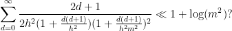
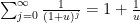
A common task in analysis is to obtain bounds on sums

or integrals

where is some simple region (such as an interval) in one or more dimensions, and is an explicit (and elementary) non-negative expression involving one or more variables (such as or , and possibly also some additional parameters. Often, one would be content with an order of magnitude upper bound such as

or

where we use (or or ) to denote the bound for some constant ; sometimes one wishes to also obtain the matching lower bound, thus obtaining

or

where is synonymous with . Finally, one may wish to obtain a more precise bound, such as

where is a quantity that goes to zero as the parameters of the problem go to infinity (or some other limit). (For a deeper dive into asymptotic notation in general, see this previous blog post.)

Here are some typical examples of such estimation problems, drawn from recent questions on MathOverflow:

• (i) (From this question) If and , is the expression

  

  finite?
• (ii) (From this question) If , how can one show that

  

• (iii) (From this question) Can one show that

  

  as for an explicit constant , and what is this constant?

Compared to other estimation tasks, such as that of controlling oscillatory integrals, exponential sums, singular integrals, or expressions involving one or more unknown functions (that are only known to lie in some function spaces, such as an space), high-dimensional geometry (or alternatively, large numbers of random variables), or number-theoretic structures (such as the primes), estimation of sums or integrals of non-negative elementary expressions is a relatively straightforward task, and can be accomplished by a variety of methods. The art of obtaining such estimates is typically not explicitly taught in textbooks, other than through some examples and exercises; it is typically picked up by analysts (or those working in adjacent areas, such as PDE, combinatorics, or theoretical computer science) as graduate students, while they work through their thesis or their first few papers in the subject.

Somewhat in the spirit of this previous post on analysis problem solving strategies, I am going to try here to collect some general principles and techniques that I have found useful for these sorts of problems. As with the previous post, I hope this will be something of a living document, and encourage others to add their own tips or suggestions in the comments.

Yoneda’s lemma as an identification of form and function: the case study of polynomials

As someone who had a relatively light graduate education in algebra, the import of Yoneda’s lemma in category theory has always eluded me somewhat; the statement and proof are simple enough, but definitely have the “abstract nonsense” flavor that one often ascribes to this part of mathematics, and I struggled to connect it to the more grounded forms of intuition, such as those based on concrete examples, that I was more comfortable with. There is a popular MathOverflow post devoted to this question, with many answers that were helpful to me, but I still felt vaguely dissatisfied. However, recently when pondering the very concrete concept of a polynomial, I managed to accidentally stumble upon a special case of Yoneda’s lemma in action, which clarified this lemma conceptually for me. In the end it was a very simple observation (and would be extremely pedestrian to anyone who works in an algebraic field of mathematics), but as I found this helpful to a non-algebraist such as myself, and I thought I would share it here in case others similarly find it helpful.

In algebra we see a distinction between a polynomial form (also known as a formal polynomial), and a polynomial function, although this distinction is often elided in more concrete applications. A polynomial form in, say, one variable with integer coefficients, is a formal expression of the form

where are coefficients in the integers, and is an indeterminate: a symbol that is often intended to be interpreted as an integer, real number, complex number, or element of some more general ring , but is for now a purely formal object. The collection of such polynomial forms is denoted , and is a commutative ring.

A polynomial form can be interpreted in any ring (even non-commutative ones) to create a polynomial function , defined by the formula

for any . This definition (2) looks so similar to the definition (1) that we usually abuse notation and conflate with . This conflation is supported by the identity theorem for polynomials, that asserts that if two polynomial forms agree at an infinite number of (say) complex numbers, thus for infinitely many , then they agree as polynomial forms (i.e., their coefficients match). But this conflation is sometimes dangerous, particularly when working in finite characteristic. For instance:

• (i) The linear forms and are distinct as polynomial forms, but agree when interpreted in the ring , since for all .
• (ii) Similarly, if is a prime, then the degree one form and the degree form are distinct as polynomial forms (and in particular have distinct degrees), but agree when interpreted in the ring , thanks to Fermat’s little theorem.
• (iii) The polynomial form has no roots when interpreted in the reals , but has roots when interpreted in the complex numbers . Similarly, the linear form has no roots when interpreted in the integers , but has roots when interpreted in the rationals .

The above examples show that if one only interprets polynomial forms in a specific ring , then some information about the polynomial could be lost (and some features of the polynomial, such as roots, may be “invisible” to that interpretation). But this turns out not to be the case if one considers interpretations in all rings simultaneously, as we shall now discuss.

If are two different rings, then the polynomial functions and arising from interpreting a polynomial form in these two rings are, strictly speaking, different functions. However, they are often closely related to each other. For instance, if is a subring of , then agrees with the restriction of to . More generally, if there is a ring homomorphism from to , then and are intertwined by the relation

which basically asserts that ring homomorphism respect polynomial operations. Note that the previous observation corresponded to the case when was an inclusion homomorphism. Another example comes from the complex conjugation automorphism on the complex numbers, in which case (3) asserts the identity

for any polynomial function on the complex numbers, and any complex number .

What was surprising to me (as someone who had not internalized the Yoneda lemma) was that the converse statement was true: if one had a function associated to every ring that obeyed the intertwining relation

for every ring homomorphism , then there was a unique polynomial form such that for all rings . This seemed surprising to me because the functions were a priori arbitrary functions, and as an analyst I would not expect them to have polynomial structure. But the fact that (4) holds for all rings and all homomorphisms is in fact rather powerful. As an analyst, I am tempted to proceed by first working with the ring of complex numbers and taking advantage of the aforementioned identity theorem, but this turns out to be tricky because does not “talk” to all the other rings enough, in the sense that there are not always as many ring homomorphisms from to as one would like. But there is in fact a more elementary argument that takes advantage of a particularly relevant (and “talkative”) ring to the theory of polynomials, namely the ring of polynomials themselves. Given any other ring , and any element of that ring, there is a unique ring homomorphism from to that maps to , namely the evaluation map

that sends a polynomial form to its evaluation at . Applying (4) to this ring homomorphism, and specializing to the element of , we conclude that

for any ring and any . If we then define to be the formal polynomial

then this identity can be rewritten as

and so we have indeed shown that the family arises from a polynomial form . Conversely, from the identity

valid for any polynomial form , we see that two polynomial forms can only generate the same polynomial functions for all rings if they are identical as polynomial forms. So the polynomial form associated to the family is unique.

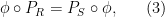
We have thus created an identification of form and function: polynomial forms are in one-to-one correspondence with families of functions obeying the intertwining relation (4). But this identification can be interpreted as a special case of the Yoneda lemma, as follows. There are two categories in play here: the category of rings (where the morphisms are ring homomorphisms), and the category of sets (where the morphisms are arbitrary functions). There is an obvious forgetful functor between these two categories that takes a ring and removes all of the algebraic structure, leaving behind just the underlying set. A collection of functions (i.e., -morphisms) for each in that obeys the intertwining relation (4) is precisely the same thing as a natural transformation from the forgetful functor to itself. So we have identified formal polynomials in as a set with natural endomorphisms of the forgetful functor:

Informally: polynomial forms are precisely those operations on rings that are respected by ring homomorphisms.

What does this have to do with Yoneda’s lemma? Well, remember that every element of a ring came with an evaluation homomorphism . Conversely, every homomorphism from to will be of the form for a unique – indeed, will just be the image of under this homomorphism. So the evaluation homomorphism provides a one-to-one correspondence between elements of , and ring homomorphisms in . This correspondence is at the level of sets, so this gives the identification

Thus our identification can be written as

which is now clearly a special case of the Yoneda lemma

that applies to any functor from a (locally small) category and any object in . And indeed if one inspects the standard proof of this lemma, it is essentially the same argument as the argument we used above to establish the identification (5). More generally, it seems to me that the Yoneda lemma is often used to identify “formal” objects with their “functional” interpretations, as long as one simultaneously considers interpretations across an entire category (such as the category of rings), as opposed to just a single interpretation in a single object of the category in which there may be some loss of information due to the peculiarities of that specific object. Grothendieck’s “functor of points” interpretation of a scheme, discussed in this previous blog post, is one typical example of this.

Inequalities, convergence, and continuity as “special deals”

The “epsilon-delta” nature of analysis can be daunting and unintuitive to students, as the heavy reliance on inequalities rather than equalities. But it occurred to me recently that one might be able to leverage the intuition one already has from “deals” – of the type one often sees advertised by corporations – to get at least some informal understanding of these concepts.

Take for instance the concept of an upper bound or a lower bound on some quantity . From an economic perspective, one could think of the upper bound as an assertion that can be “bought” for units of currency, and the lower bound can similarly be viewed as an assertion that can be “sold” for units of currency. Thus for instance, a system of inequalities and equations like

could be viewed as analogous to a currency rate exchange board, of the type one sees for instance in airports:

Currency	We buy at	We sell at
	–
	–

Someone with an eye for spotting “deals” might now realize that one can actually buy for units of currency rather than , by purchasing one copy each of and for units of currency, then selling off to recover units of currency back. In more traditional mathematical language, one can improve the upper bound to by taking the appropriate linear combination of the inequalities , , and . More generally, this way of thinking is useful when faced with a linear programming situation (and of course linear programming is a key foundation for operations research), although this analogy begins to break down when one wants to use inequalities in a more non-linear fashion.

Asymptotic estimates such as (also often written or ) can be viewed as some sort of liquid market in which can be used to purchase , though depending on market rates, one may need a large number of units of in order to buy a single unit of . An asymptotic estimate like represents an economic situation in which is so much more highly desired than that, if one is a patient enough haggler, one can eventually convince someone to give up a unit of for even just a tiny amount of .

When it comes to the basic analysis concepts of convergence and continuity, one can similarly view these concepts as various economic transactions involving the buying and selling of accuracy. One could for instance imagine the following hypothetical range of products in which one would need to spend more money to obtain higher accuracy to measure weight in grams:

Object	Accuracy	Price
Low-end kitchen scale	gram
High-end bathroom scale	grams
Low-end lab scale	grams
High-end lab scale	grams

The concept of convergence of a sequence to a limit could then be viewed as somewhat analogous to a rewards program, of the type offered for instance by airlines, in which various tiers of perks are offered when one hits a certain level of “currency” (e.g., frequent flyer miles). For instance, the convergence of the sequence to its limit offers the following accuracy “perks” depending on one’s level in the sequence:

Status	Accuracy benefit	Eligibility
Basic status
Bronze status
Silver status
Gold status

With this conceptual model, convergence means that any status level of accuracy can be unlocked if one’s number of “points earned” is high enough.

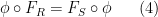
In a similar vein, continuity becomes analogous to a conversion program, in which accuracy benefits from one company can be traded in for new accuracy benefits in another company. For instance, the continuity of the function at the point can be viewed in terms of the following conversion chart:

Accuracy benefit of to trade in	Accuracy benefit of obtained

Again, the point is that one can purchase any desired level of accuracy of provided one trades in a suitably high level of accuracy of .

At present, the above conversion chart is only available at the single location . The concept of uniform continuity can then be viewed as an advertising copy that “offer prices are valid in all store locations”. In a similar vein, the concept of equicontinuity for a class of functions is a guarantee that “offer applies to all functions in the class , without any price discrimination. The combined notion of uniform equicontinuity is then of course the claim that the offer is valid in all locations and for all functions.

In a similar vein, differentiability can be viewed as a deal in which one can trade in accuracy of the input for approximately linear behavior of the output; to oversimplify slightly, smoothness can similarly be viewed as a deal in which one trades in accuracy of the input for high-accuracy polynomial approximability of the output. Measurability of a set or function can be viewed as a deal in which one trades in a level of resolution for an accurate approximation of that set or function at the given resolution. And so forth.

Perhaps readers can propose some other examples of mathematical concepts being re-interpreted as some sort of economic transaction?

Special relativity and Middle-Earth

This post is an unofficial sequel to one of my first blog posts from 2007, which was entitled “Quantum mechanics and Tomb Raider“.

One of the oldest and most famous allegories is Plato’s allegory of the cave. This allegory centers around a group of people chained to a wall in a cave that cannot see themselves or each other, but only the two-dimensional shadows of themselves cast on the wall in front of them by some light source they cannot directly see. Because of this, they identify reality with this two-dimensional representation, and have significant conceptual difficulties in trying to view themselves (or the world as a whole) as three-dimensional, until they are freed from the cave and able to venture into the sunlight.

There is a similar conceptual difficulty when trying to understand Einstein’s theory of special relativity (and more so for general relativity, but let us focus on special relativity for now). We are very much accustomed to thinking of reality as a three-dimensional space endowed with a Euclidean geometry that we traverse through in time, but in order to have the clearest view of the universe of special relativity it is better to think of reality instead as a four-dimensional spacetime that is endowed instead with a Minkowski geometry, which mathematically is similar to a (four-dimensional) Euclidean space but with a crucial change of sign in the underlying metric. Indeed, whereas the distance between two points in Euclidean space is given by the three-dimensional Pythagorean theorem

under some standard Cartesian coordinate system of that space, and the distance in a four-dimensional Euclidean space would be similarly given by

under a standard four-dimensional Cartesian coordinate system , the spacetime interval in Minkowski space is given by

(though in many texts the opposite sign convention is preferred) in spacetime coordinates , where is the speed of light. The geometry of Minkowski space is then quite similar algebraically to the geometry of Euclidean space (with the sign change replacing the traditional trigonometric functions , etc. by their hyperbolic counterparts , and with various factors involving “” inserted in the formulae), but also has some qualitative differences to Euclidean space, most notably a causality structure connected to light cones that has no obvious counterpart in Euclidean space.

That said, the analogy between Minkowski space and four-dimensional Euclidean space is strong enough that it serves as a useful conceptual aid when first learning special relativity; for instance the excellent introductory text “Spacetime physics” by Taylor and Wheeler very much adopts this view. On the other hand, this analogy doesn’t directly address the conceptual problem mentioned earlier of viewing reality as a four-dimensional spacetime in the first place, rather than as a three-dimensional space that objects move around in as time progresses. Of course, part of the issue is that we aren’t good at directly visualizing four dimensions in the first place. This latter problem can at least be easily addressed by removing one or two spatial dimensions from this framework – and indeed many relativity texts start with the simplified setting of only having one spatial dimension, so that spacetime becomes two-dimensional and can be depicted with relative ease by spacetime diagrams – but still there is conceptual resistance to the idea of treating time as another spatial dimension, since we clearly cannot “move around” in time as freely as we can in space, nor do we seem able to easily “rotate” between the spatial and temporal axes, the way that we can between the three coordinate axes of Euclidean space.

With this in mind, I thought it might be worth attempting a Plato-type allegory to reconcile the spatial and spacetime views of reality, in a way that can be used to describe (analogues of) some of the less intuitive features of relativity, such as time dilation, length contraction, and the relativity of simultaneity. I have (somewhat whimsically) decided to place this allegory in a Tolkienesque fantasy world (similarly to how my previous allegory to describe quantum mechanics was phrased in a world based on the computer game “Tomb Raider”). This is something of an experiment, and (like any other analogy) the allegory will not be able to perfectly capture every aspect of the phenomenon it is trying to represent, so any feedback to improve the allegory would be appreciated.

An improvement to Bennett’s inequality for the Poisson distribution

If , a Poisson random variable with mean is a random variable taking values in the natural numbers with probability distribution

One is often interested in bounding upper tail probabilities

for , or lower tail probabilities

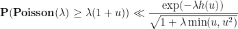
for . A standard tool for this is Bennett’s inequality:

Proposition 1 (Bennett’s inequality) One has

for and

for , where

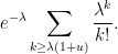
From the Taylor expansion for we conclude Gaussian type tail bounds in the regime (and in particular when (in the spirit of the Chernoff, Bernstein, and Hoeffding inequalities). but in the regime where is large and positive one obtains a slight gain over these other classical bounds (of type, rather than ).

Proof: We use the exponential moment method. For any , we have from Markov’s inequality that

A standard computation shows that the moment generating function of the Poisson distribution is given by

and hence

For , it turns out that the right-hand side is optimized by setting , in which case the right-hand side simplifies to . This proves the first inequality; the second inequality is proven similarly (but now and are non-positive rather than non-negative).

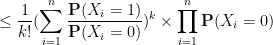
Remark 2 Bennett’s inequality also applies for (suitably normalized) sums of bounded independent random variables. In some cases there are direct comparison inequalities available to relate those variables to the Poisson case. For instance, suppose is the sum of independent Boolean variables of total mean and with for some . Then for any natural number , we have

As such, for small, one can efficiently control the tail probabilities of in terms of the tail probability of a Poisson random variable of mean close to ; this is of course very closely related to the well known fact that the Poisson distribution emerges as the limit of sums of many independent boolean variables, each of which is non-zero with small probability. See this paper of Bentkus and this paper of Pinelis for some further useful (and less obvious) comparison inequalities of this type.

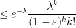
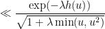
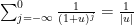
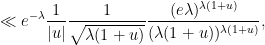
In this note I wanted to record the observation that one can improve the Bennett bound by a small polynomial factor once one leaves the Gaussian regime , in particular gaining a factor of when . This observation is not difficult and is implicitly in the literature (one can extract it for instance from the much more general results of this paper of Talagrand, and the basic idea already appears in this paper of Glynn), but I was not able to find a clean version of this statement in the literature, so I am placing it here on my blog. (But if a reader knows of a reference that basically contains the bound below, I would be happy to know of it.)

Proposition 3 (Improved Bennett’s inequality) One has

for and

for .

Proof: We begin with the first inequality. We may assume that , since otherwise the claim follows from the usual Bennett inequality. We expand out the left-hand side as

Observe that for that

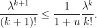
Thus the sum is dominated by the first term times a geometric series . We can thus bound the left-hand side by

By the Stirling approximation, this is

The expression inside the supremum is decreasing in for , thus we can bound it by

which simplifies to

after a routine calculation.

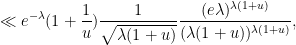
Now we turn to the second inequality. As before we may assume that . We first dispose of a degenerate case in which . Here the left-hand side is just

and the right-hand side is comparable to

Since is negative and 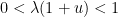, we see that the right-hand side is , and the estimate holds in this case.

It remains to consider the regime where and . The left-hand side expands as

The sum is dominated by the first term times a geometric series . The maximal is comparable to , so we can bound the left-hand side by

Using the Stirling approximation as before we can bound this by

which simplifies to

after a routine calculation.

The same analysis can be reversed to show that the bounds given above are basically sharp up to constants, at least when (and ) are large.

A Bayesian probability worksheet

This is a spinoff from the previous post. In that post, we remarked that whenever one receives a new piece of information , the prior odds between an alternative hypothesis and a null hypothesis is updated to a posterior odds , which can be computed via Bayes’ theorem by the formula

where is the likelihood of this information under the alternative hypothesis , and is the likelihood of this information under the null hypothesis . If there are no other hypotheses under consideration, then the two posterior probabilities , must add up to one, and so can be recovered from the posterior odds by the formulae

This gives a straightforward way to update one’s prior probabilities, and I thought I would present it in the form of a worksheet for ease of calculation:

A PDF version of the worksheet and instructions can be found here. One can fill in this worksheet in the following order:

1. In Box 1, one enters in the precise statement of the null hypothesis .
2. In Box 2, one enters in the precise statement of the alternative hypothesis . (This step is very important! As discussed in the previous post, Bayesian calculations can become extremely inaccurate if the alternative hypothesis is vague.)
3. In Box 3, one enters in the prior probability (or the best estimate thereof) of the null hypothesis .
4. In Box 4, one enters in the prior probability (or the best estimate thereof) of the alternative hypothesis . If only two hypotheses are being considered, we of course have .
5. In Box 5, one enters in the ratio between Box 4 and Box 3.
6. In Box 6, one enters in the precise new information that one has acquired since the prior state. (As discussed in the previous post, it is important that all relevant information – both supporting and invalidating the alternative hypothesis – are reported accurately. If one cannot be certain that key information has not been withheld to you, then Bayesian calculations become highly unreliable.)
7. In Box 7, one enters in the likelihood (or the best estimate thereof) of the new information under the null hypothesis .
8. In Box 8, one enters in the likelihood (or the best estimate thereof) of the new information under the null hypothesis . (This can be difficult to compute, particularly if is not specified precisely.)
9. In Box 9, one enters in the ratio betwen Box 8 and Box 7.
10. In Box 10, one enters in the product of Box 5 and Box 9.
11. (Assuming there are no other hypotheses than and ) In Box 11, enter in divided by plus Box 10.
12. (Assuming there are no other hypotheses than and ) In Box 12, enter in Box 10 divided by plus Box 10. (Alternatively, one can enter in minus Box 11.)

To illustrate this procedure, let us consider a standard Bayesian update problem. Suppose that a given point in time, of the population is infected with COVID-19. In response to this, a company mandates COVID-19 testing of its workforce, using a cheap COVID-19 test. This test has a chance of a false negative (testing negative when one has COVID) and a chance of a false positive (testing positive when one does not have COVID). An employee takes the mandatory test, which turns out to be positive. What is the probability that actually has COVID?

We can fill out the entries in the worksheet one at a time:

• Box 1: The null hypothesis is that does not have COVID.
• Box 2: The alternative hypothesis is that does have COVID.
• Box 3: In the absence of any better information, the prior probability of the null hypothesis is , or .
• Box 4: Similarly, the prior probability of the alternative hypothesis is , or .
• Box 5: The prior odds are .
• Box 6: The new information is that has tested positive for COVID.
• Box 7: The likelihood of under the null hypothesis is , or (the false positive rate).
• Box 8: The likelihood of under the alternative is , or (one minus the false negative rate).
• Box 9: The likelihood ratio is .
• Box 10: The product of Box 5 and Box 9 is approximately .
• Box 11: The posterior probability is approximately .
• Box 12: The posterior probability is approximately .

The filled worksheet looks like this:

Perhaps surprisingly, despite the positive COVID test, the employee only has a chance of actually having COVID! This is due to the relatively large false positive rate of this cheap test, and is an illustration of the base rate fallacy in statistics.

We remark that if we switch the roles of the null hypothesis and alternative hypothesis, then some of the odds in the worksheet change, but the ultimate conclusions remain unchanged:

So the question of which hypothesis to designate as the null hypothesis and which one to designate as the alternative hypothesis is largely a matter of convention.

Now let us take a superficially similar situation in which a mother observers her daughter exhibiting COVID-like symptoms, to the point where she estimates the probability of her daughter having COVID at . She then administers the same cheap COVID-19 test as before, which returns positive. What is the posterior probability of her daughter having COVID?

One can fill out the worksheet much as before, but now with the prior probability of the alternative hypothesis raised from to (and the prior probablity of the null hypothesis dropping from to ). One now gets that the probability that the daughter has COVID has increased all the way to :

Thus we see that prior probabilities can make a significant impact on the posterior probabilities.

Now we use the worksheet to analyze an infamous probability puzzle, the Monty Hall problem. Let us use the formulation given in that Wikipedia page:

Problem 1 Suppose you’re on a game show, and you’re given the choice of three doors: Behind one door is a car; behind the others, goats. You pick a door, say No. 1, and the host, who knows what’s behind the doors, opens another door, say No. 3, which has a goat. He then says to you, “Do you want to pick door No. 2?” Is it to your advantage to switch your choice?

For this problem, the precise formulation of the null hypothesis and the alternative hypothesis become rather important. Suppose we take the following two hypotheses:

• Null hypothesis : The car is behind door number 1, and no matter what door you pick, the host will randomly reveal another door that contains a goat.
• Alternative hypothesis : The car is behind door number 2 or 3, and no matter what door you pick, the host will randomly reveal another door that contains a goat.

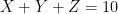
Assuming the prizes are distributed randomly, we have and . The new information is that, after door 1 is selected, door 3 is revealed and shown to be a goat. After some thought, we conclude that is equal to (the host has a fifty-fifty chance of revealing door 3 instead of door 2) but that is also equal to (if the car is behind door 2, the host must reveal door 3, whereas if the car is behind door 3, the host cannot reveal door 3). Filling in the worksheet, we see that the new information does not in fact alter the odds, and the probability that the car is not behind door 1 remains at 2/3, so it is advantageous to switch.

However, consider the following different set of hypotheses:

• Null hypothesis : The car is behind door number 1, and if you pick the door with the car, the host will reveal another door to entice you to switch. Otherwise, the host will not reveal a door.
• Alternative hypothesis : The car is behind door number 2 or 3, and if you pick the door with the car, the host will reveal another door to entice you to switch. Otherwise, the host will not reveal a door.

Here we still have and , but while remains equal to , has dropped to zero (since if the car is not behind door 1, the host will not reveal a door). So now has increased all the way to , and it is not advantageous to switch! This dramatically illustrates the importance of specifying the hypotheses precisely. The worksheet is now filled out as follows:

Finally, we consider another famous probability puzzle, the Sleeping Beauty problem. Again we quote the problem as formulated on the Wikipedia page:

Problem 2 Sleeping Beauty volunteers to undergo the following experiment and is told all of the following details: On Sunday she will be put to sleep. Once or twice, during the experiment, Sleeping Beauty will be awakened, interviewed, and put back to sleep with an amnesia-inducing drug that makes her forget that awakening. A fair coin will be tossed to determine which experimental procedure to undertake:

• If the coin comes up heads, Sleeping Beauty will be awakened and interviewed on Monday only.
• If the coin comes up tails, she will be awakened and interviewed on Monday and Tuesday.
• In either case, she will be awakened on Wednesday without interview and the experiment ends.

Any time Sleeping Beauty is awakened and interviewed she will not be able to tell which day it is or whether she has been awakened before. During the interview Sleeping Beauty is asked: “What is your credence now for the proposition that the coin landed heads?”‘

Here the situation can be confusing because there are key portions of this experiment in which the observer is unconscious, but nevertheless Bayesian probability continues to operate regardless of whether the observer is conscious. To make this issue more precise, let us assume that the awakenings mentioned in the problem always occur at 8am, so in particular at 7am, Sleeping beauty will always be unconscious.

Here, the null and alternative hypotheses are easy to state precisely:

• Null hypothesis : The coin landed tails.
• Alternative hypothesis : The coin landed heads.

The subtle thing here is to work out what the correct prior state is (in most other applications of Bayesian probability, this state is obvious from the problem). It turns out that the most reasonable choice of prior state is “unconscious at 7am, on either Monday or Tuesday, with an equal chance of each”. (Note that whatever the outcome of the coin flip is, Sleeping Beauty will be unconscious at 7am Monday and unconscious again at 7am Tuesday, so it makes sense to give each of these two states an equal probability.) The new information is then

• New information : One hour after the prior state, Sleeping Beauty is awakened.

With this formulation, we see that , , and , so on working through the worksheet one eventually arrives at , so that Sleeping Beauty should only assign a probability of to the event that the coin landed as heads.

There are arguments advanced in the literature to adopt the position that should instead be equal to , but I do not see a way to interpret them in this Bayesian framework without a substantial alteration to either the notion of the prior state, or by not presenting the new information properly.

If one has multiple pieces of information that one wishes to use to update one’s priors, one can do so by filling out one copy of the worksheet for each new piece of information, or by using a multi-row version of the worksheet using such identities as

We leave the details of these variants of the Bayesian update problem to the interested reader. The only thing I will note though is that if a key piece of information is withheld from the person filling out the worksheet, for instance if that person relies exclusively on a news source that only reports information that supports the alternative hypothesis and omits information that debunks it, then the outcome of the worksheet is likely to be highly inaccurate, and one should only perform a Bayesian analysis when one has a high confidence that all relevant information (both favorable and unfavorable to the alternative hypothesis) is being reported to the user.